Numerical study of staggered fermion on anisotropic lattices

Abstract

We study calibration procedures of the staggered quarks on anisotropic lattices in the quenched approximation and in $N_{f}=2$ dynamical simulations. For the calibration conditions we adopt the hadronic radii $r_{0}$ and the meson masses in the temporal and spatial directions. On the quenched lattice, we calibrate the quark field and compare the result with the result determined using the meson dispersion relation. In dynamical simulations, we determine the anisotropy parameters $\gamma_{G}$ and $\gamma_{F}$ simultaneously within 1% accuracy at renormalized anisotropy $\xi=a_{s}/a_{t}=4$.

1 Introduction

Anisotropic lattices realize small temporal lattice spacings while keeping modest computational costs. The technique is useful in various fields of lattice QCD simulation: At finite temperature the large number of degrees of freedom in Euclidean time direction leads large number of Matsubara frequencies, which is efficient for calculation of the equation of state [1] and for analyses of temporal correlation functions [2, 3, 4]. The large temporal cutoff is important for relativistic formulations of heavy quarks on lattices [5]. It is also convenient for the correlators in which noises quickly grow as time such as glueballs [4, 6] and negative parity baryons [7].

However, uncertainties of anisotropy parameters bring additional errors into the observed quantities. For precise calculations, we need to tune anisotropy parameters with good statistical accuracies and to control the systematic errors in the continuum extrapolations. In this work we discuss the tuning procedures of anisotropy parameters for the staggered fermions in the quenched and dynamical QCD simulations. Our goal is to tune anisotropy parameters within 1% statistical errors at each set of $\beta$ and $m_{0}$. In the following, we focus on lattices with the renormalized anisotropy $\xi=a_{s}/a_{t}=4$.

2 Lattice action

In the numerical simulations, we adopt Wilson gauge and staggered quark actions on anisotropic lattices. The Staggered quarks have several advantages over the Wilson-type quarks in studies related to the chiral symmetry and in simulations at lighter quark masses. The gauge action is

$$S_{G} = \beta\sum_{x}\left\{\sum_{i<j}^{3}\frac{1}{\gamma_{G}}\left[1-\frac{1}{3}\mathop{\rm Re}\mathop{\rm Tr}U_{ij}(x)\right]+\right.$$ (1)

$$\left.\sum_{i}^{3}\gamma_{G}\left[1-\frac{1}{3}\mathop{\rm Re}\mathop{\rm Tr}U_{i4}(x)\right]\right\},$$

where $\gamma_{G}$ is the bare gauge anisotropy parameter. The quark action is defined as

$$S_{F}=\sum_{x,y}\bar{\chi}(x)K(x,y)\chi(y).$$ (2)

$$K(x,y)=\delta_{x,y}$$ (3)

$$-\gamma_{F}\kappa_{\sigma}\eta_{4}(x)\left[U_{4}(x)\delta_{x,y-\hat{4}}-U^{\dagger}_{4}(x-\hat{4})\delta_{x,y+\hat{4}}\right]$$

$$-\kappa_{\sigma}\sum_{i}\eta_{\mu}(x)\left[U_{i}(x)\delta_{x,y-\hat{i}}-U^{\dagger}_{i}(x-\hat{i})\delta_{x,y+\hat{i}}\right],$$

where $\gamma_{F}$ is a bare fermionic anisotropy parameter, $\eta_{\mu}(x)$ the staggered phase, $\kappa_{\sigma}=1/2m_{0}$ with $m_{0}$ the bare quark mass in spatial lattice units.

Although these anisotropic lattice actions have been adopted in Ref.[8], they did not discuss the systematic uncertainties due to the anisotropy to the sufficient level for precision computations.

3 Calibration procedures

The anisotropy parameters $\gamma_{G}$ and $\gamma_{F}$ should be tuned so that the physical isotropy condition, $\xi_{G}(\gamma_{G}^{*},\gamma_{F}^{*})=\xi_{F}(\gamma_{G}^{*},\gamma_{F}^{*})=\xi$ holds at each set of $\beta$ and $m_{0}$, where $\xi_{G}(\gamma_{G},\gamma_{F})$ and $\xi_{F}(\gamma_{G},\gamma_{F})$ are the renormalized anisotropies defined through the gauge and quark observables, respectively. In quenched simulations, one can firstly determine the $\gamma_{G}$ independently of $\gamma_{F}$, and then tune $\gamma_{F}$ for fixed $\gamma_{G}$. On the other hand, in dynamical simulations, $\gamma_{G}$ and $\gamma_{F}$ need to be tuned simultaneously.

3.1 Gauge sector

For the calibration in the gauge sector, we define $\xi_{G}(\gamma_{G},\gamma_{F})$ through the hadronic radii $r_{0}$ [9] in the spatial and temporal directions. Since we set the lattice scale via $r_{0}$, the physical anisotropy is kept in the continuum extrapolation. This is an advantage to avoid that the systematic errors brought by the anisotropic lattice remain in the continuum limit.

The value of $r_{0}$ is defined with the static $q$-$\bar{q}$ potential through the relation $r_{0}^{2}F(r_{0})=1.65$, where $F(r)$ is the force between quarks. Then $\xi_{G}$ is defined with the ratio of $r_{0}$’s in the temporal and spatial directions: $\xi_{G}=r_{0}^{(t)}/r_{0}^{(x)}$.

In quenched simulations, we can apply the Lüscher-Weisz noise reduction technique [10] and determine $\xi_{G}$ at 0.2% level of accuracy [12]. In dynamical simulations, we instead apply the smearing technique to the anisotropic three-dimensional planes which enables determination of $\xi_{G}$ at 1% level of accurately.

3.2 Quark sector

In the fermion sector, we define $\xi_{F}$ with the ratio of meson masses in temporal and spatial directions: $\xi_{F}=m_{h}^{(z)}/m_{h}^{(t)}$ [2]. We use the pseudoscalar channel, since in that channel the oscillating components of the correlators disappear quickly and hence statistical errors of masses are small.

Alternative definition of the $\xi_{F}$ makes use of the meson dispersion relation [11],

$$E^{2}(\mbox{\boldmath$p$})=m^{2}+\mbox{\boldmath$p$}^{2}/\xi_{F}^{2}.$$ (4)

Here $E(\mbox{\boldmath$p$})$ and $m$ are in temporal lattice units and $p$ is in spatial lattice units, and hence $\xi_{F}$ appears. $p_{i}=2\pi n_{i}/L_{i}$ ($i=$1,2,3), where $L_{i}$ is lattice size in $i$-th direction. We use $\mbox{\boldmath$n$}=(0,0,0),(0,0,1)$ to define $\xi_{F}$.

At present stage of this work, we adopt the former procedure, with the ratio of the temporal and spatial meson masses, as the main calibration procedure for the quark field, because of smaller statistical uncertainties than the latter definition. In quenched simulation, we compare the results with these two procedures.

4 Numerical results of calibration

4.1 Quenched simulation

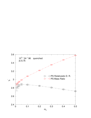
Figure 1: The result of calibration of the staggered quark field in the quenched simulation.

The simulation is performed on a $12^{2}\times 24\times 96$ lattice at $\beta=5.75$ and $\gamma_{G}=3.136$ which correspond to the spatial cutoff $a_{\sigma}^{-1}=$1.1 GeV and the renormalized anisotropy $\xi_{G}=4$ [12]. The statistics are 224 configurations. The bare quark mass range is from 0.01 to 0.5 which corresponds to the range $m_{PS}/m_{V}$ from 0.33 to 0.90.

We calculate the meson mass ratio at several values of $\gamma_{F}$ and interpolate them to $\gamma_{F}^{*}$ at which $\xi_{F}=4$ holds. The result is displayed in Fig. 1. For our lightest quark mass case, $\gamma_{F}^{*}$ is determined within 0.5% statistical error.

In Fig. 1, we also show the result of calibration using the meson dispersion relation. The results of two procedures are consistent only in vary light quark mass region. To understand the discrepancies of two procedures and large change of $\gamma_{F}^{*}$ from the calibration with mass ratio at larger quark mass region are subjects of future work.

4.2 dynamical simulation

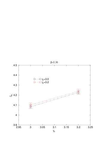
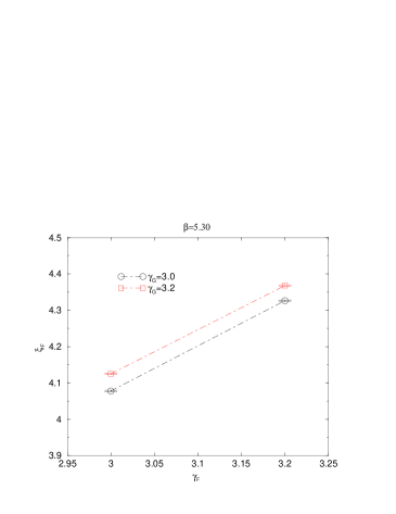
Figure 2: The result of calibration in the dynamical simulation at $\beta=5.3$, $m_{0}=0.1$. The top and bottom panel show the dependences of $\gamma_{G}$ on $\xi_{G}$ and $\gamma_{F}$ on $\xi_{F}$, respectively.

The simulation is performed with R-algorithm with $N_{f}=2$ on lattices of the size $10^{2}\times 20\times 80$ at 4 values of $\beta$ from 5.3 to 5.45 and the quark mass $m_{0}=0.1$. The statistics are from 300 to 800 trajectories after 200 for thermalization. In the following we present only the result at $\beta=5.3$ on which the spatial cutoff is $a_{\sigma}^{-1}=$ 0.69 GeV and $m_{PS}/m_{V}=0.6$.

We determine $\gamma_{G}^{*}$ and $\gamma_{F}^{*}$ by a linear interpolation to $\xi=4$ using the 6 parameter sets of ($\gamma_{G}$,$\gamma_{F}$) assuming the following relations:

$$\xi_{G} = a_{0}+a_{1}(\gamma_{G}-\gamma_{G}^{*})+a_{2}(\gamma_{F}-\gamma_{F}^{*}),$$

$$\xi_{F} = b_{0}+b_{1}(\gamma_{G}-\gamma_{G}^{*})+b_{2}(\gamma_{F}-\gamma_{F}^{*}).$$ (5)

The result of calibration with the meson mass ratio is presented in Fig.2.

The $\chi^{2}$ fit results in $[a_{0},a_{1},a_{2}]=[4.000(24),0.702(92),0.075(92)]$, $[b_{0},b_{1},b_{2}]=[4.000(28),0.220(08),1.225(08)]$. We find that $\xi_{F}$ has small dependence on $\gamma_{G}$ and $\xi_{G}$ on $\gamma_{F}$. By solving Eq. (5), we obtain $\gamma_{G}^{*}=2.885(35)$, $\gamma_{F}^{*}=2.955(31)$. We can tune the parameters $\gamma_{G}$ and $\gamma_{F}$ with the 1% level of statistical errors.

This calculation was done on a Hitachi SR8000 at KEK. H.M. and T.U. thank JSPS for Young Scientists for financial support.

References

- [1] Y. Namekawa et al., Phys. Rev. D64 (2001) 074507.
- [2] QCD-TARO Collaboration, Phys. Rev. D63 (2001) 054501; T. Umeda et al., Int. J. Mod. Phys. A 16 (2001) 2215.
- [3] T. Umeda, K. Nomura, H. Matsufuru, hep-lat/0211003.
- [4] N. Ishii, H. Suganuma, and H. Matsufuru, Phys. Rev. D 66 (2002) 014507; ibid. 66 (2002) 094506.
- [5] J. Harada et al., Phys. Rev. D64 (2001) 074501; J. Harada et al., ibid. 66 (2002) 014509.
- [6] C. J. Morningstar et al., Phys. Rev. D60 (1999) 034509.
- [7] Y. Nemoto et al., hep-lat/0302013.
- [8] L. Levkova et al., Nucl. Phys. B (Proc. Suppl.) 106 (2002) 218.
- [9] R. Sommer, Nucl. Phys. B411 (1994) 839.
- [10] M. Lüscher and P. Weisz, JHEP 0109 (2001) 010.
- [11] T. Umeda et al. (CP-PACS Collaboration), Phys. Rev. D68 (2003) 034503.
- [12] H. Matsufuru et al., these proceedings.