Anisotropic lattices for precision computations in heavy flavor physics

Abstract

We study the anisotropic lattice QCD for precision computations of heavy-light matrix elements. Our previous study in which the lattices are calibrated with a few percent accuracy has already given results comparable to the existing calculations. This suggests that even higher precision may be achieved by a more precise calibration of anisotropic lattices. We describe our strategy to tune the gauge and quark parameters with accuracies much less than 1 % in the quenched approximation.

1 Introduction

Recent experimental progress at $B$ factories suggests that precise computation of hadronic matrix elements in lattice QCD is a key to the search for signals of new physics in flavor physics. However, HQET or the relativistic approaches still suffer from perturbative and/or discretization errors, which are typically of order of 10%. We therefore need yet another framework of the heavy quark in which one should be able to (i) take the continuum limit, (ii) compute the parameters in the action and the operators nonperturbatively, (iii) and compute the matrix elements with a modest computational cost.

As a candidate of framework which fulfills these conditions, we investigate the anisotropic lattice on which the temporal lattice spacing $a_{\tau}$ is finer than the spatial one $a_{\sigma}$ [1, 2, 3]. The anisotropic lattice approach evidently satisfies above conditions (i) and (iii). Our expectation is that on anisotropic lattices the mass dependence of the parameters becomes so mild that one can adopt coefficients determined nonperturbatively at massless limit. For precise computations of heavy-light matrix elements, we also need to control all the systematic errors in the extrapolations to the continuum limit. Whether these promises will be practically satisfied should be examined numerically.

So far we have investigated the feasibility of the approach in the quenched approximation and with the tree-level tadpole improvement for the $O(a)$ improved Wilson quark action [1, 2, 3, 4]. As will be summarized in Sec. 3, the results have been encouraging for further development in this direction. Therefore we have started the second stage of the study of the anisotropic lattice for heavy quarks. In this stage, we perform fully nonperturbative $O(a)$ improvement and aim at $O(2\%)$ computations of matrix elements in quenched approximation. To this end, we need to perform the calibrations with accuracies much less than 1 %. We describe our strategy to tune the gauge and quark parameters to this level in the quenched approximation.

2 Anisotropic lattice quark action

Our heavy quark formulation basically follows the Fermilab approach [5] but is formulated on the anisotropic lattices [1, 6]. The quark action is represented as

$$S_{F} = \sum_{x,y}\bar{\psi}(x)K(x,y)\psi(y),$$ (1)

$$K(x,y)\!\!\! = \!\!\!\delta_{x,y}-\kappa_{\tau}\left[\ \ (1-\gamma_{4})U_{4}(x)\delta_{x+\hat{4},y}\right.$$ (2)

$$\hskip 28.45274pt+\left.(1+\gamma_{4})U_{4}^{{\dagger}}(x-\hat{4})\delta_{x-\hat{4},y}\right]$$

$$-\kappa_{\sigma}{\textstyle\sum_{i}}\left[\ \ (r-\gamma_{i})U_{i}(x)\delta_{x+\hat{i},y}\right.$$

$$\hskip 28.45274pt+\left.(r+\gamma_{i})U_{i}^{{\dagger}}(x-\hat{i})\delta_{x-\hat{i},y}\right]$$

$$-\kappa_{\sigma}c_{E}{\textstyle\sum_{i}}\sigma_{4i}F_{4i}(x)\delta_{x,y}$$

$$-r\kappa_{\sigma}c_{B}{\textstyle\sum_{i>j}}\sigma_{ij}F_{ij}(x)\delta_{x,y},$$

where $\kappa_{\sigma}$ and $\kappa_{\tau}$ are the spatial and temporal hopping parameters, $r$ the spatial Wilson parameter and $c_{E}$ and $c_{B}$ the clover coefficients. For a given $\kappa_{\sigma}$, in principle, the four parameters $\gamma_{F}\equiv\kappa_{\tau}/\kappa_{\sigma}$, $r$, $c_{E}$ and $c_{B}$ should be tuned so that the Lorentz invariance holds up to discretization errors of $O(a^{2})$. We can set $r=1/\xi$ without loss of generality [1, 5].

In the first stage of this work, we tuned only the bare anisotropy $\gamma_{F}$ nonperturbatively and applied the tree-level tadpole-improvement to $c_{E}$ and $c_{B}$: $c_{E}=1/u_{\sigma}u_{\tau}^{2}$, $c_{B}=1/u_{\sigma}^{3}$. In the second stage, however, we need to perform the nonperturbative tuning of all the three parameters $\gamma_{F}$, $c_{E}$, and $c_{B}$, as well as the parameters of the operators which appear in the matrix elements.

3 Summary of the first stage results

In the first stage of this work, we have obtained the following results in the quenched approximation.

One-loop perturbative calculation [1]: Renormalization factors of heavy-light bilinears and quark rest mass at $m_{Q}a_{\sigma}\sim 1$, $m_{Q}\ll a_{\tau}^{-1}$ are calculated in the one-loop perturbation theory. The $m_{Q}a_{\tau}$ dependence of the coefficients are well approximated with linear form and this means that the quark mass dependence can be controlled.

Numerical simulation in the quenched approximation [2]: The mass dependent tuning of $\gamma_{F}$ is performed with meson dispersion relation. Quark mass dependence is small for $m_{q}a_{\tau}\ll 1$ and well fitted to a linear form in $(m_{q}a_{\tau})^{2}$.

Test of relativity relation [3]: Heavy-light meson dispersion relation is computed with $\gamma_{F}=\gamma_{F}(m_{q}=0)$. The relativity relation well holds for the region $m_{q}a_{\tau}\ll 1$ while $m_{q}a_{\sigma}\stackrel{{\scriptstyle>}}{{\scriptstyle\sim}}1$.

Application to the decay constant [4]. Around the charm quark mass, the heavy-light decay constant is calculated. The result is consistent with previous works. This implies that our program successfully works at least for computations at $O(10\%)$ accuracy.

These results are encouraging for further development along this direction.

4 Strategy for the second stage

The goal of the second stage is to perform the quenched computations of heavy-light matrix elements within a few percent uncertainties. To achieve this precision, the calibration must be performed to the level of accuracy much less than one percent both for the gauge and quark fields.

4.1 Calibration of gauge field

In the quenched approximation, the calibration of gauge field can be performed independently of the quark field. The elaborated work by Klassen [7], the $O(1\%)$ level calibration for the Wilson action, is no longer enough for the present purposes. For more precise calibration of gauge field, we need to measure the static quark potential very accurately. For this purpose, we adopt the Lüscher-Weisz noise reduction technique [8].

We define the renormalized anisotropy $\xi_{G}$ through the hadronic radius $r_{0}$ measured in the spatial and the temporal directions. Since we carry out the continuum extrapolation in terms of the lattice scale set by $r_{0}$, the renormalized anisotropy is kept fixed during the extrapolation. This procedure prevents the systematic uncertainties due to the anisotropy from remaining in the continuum limit.

Figure 1 shows a result of static quark potential at $\beta=5.8$ and $\gamma_{G}=3.10$: the displayed data are the force between static quarks separated in the spatial (coarse) and temporal (fine) directions. The values of $r_{0}$, which is defined through the relation $r_{0}^{2}F(r_{0})=1.65$, are determined within 0.2% statistical errors. Fig. 2 exhibits the determination of $\gamma_{G}^{*}$, which satisfies $\xi_{G}(\gamma_{G}^{*})=\xi=4$, at $\beta=5.75$. A linear $\chi^{2}$ fit gives $\gamma_{G}^{*}=3.1399(52)$, which satisfies the required accuracy. The calibration in wider range of $\beta$ at $\xi=4$ is in progress.

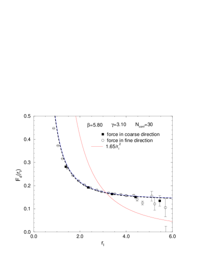
Figure 1: Determination of gauge field anisotropy.

Figure 2: Calibration of gauge field at $\beta=5.75$.

4.2 Calibration of quark field

We need to calibrate the parameters in the action, $\gamma_{F}$, $c_{E}$, $c_{B}$, to the level which enables computations of matrix elements within a few percent accuracy. We also need to perform the nonperturbative renormalization of the operators such as the heavy-light axial current. The nonperturbative renormalization technique [10, 11, 12] is one of the most powerful methods to perform such a program. Since our expectation is that the result of tuning near the massless limit can be applied to the heavy quark region if $m_{Q}a_{\tau}\ll 1$ holds, the technique can be applied with a little modification in accord with the anisotropic lattice.

The Schrödinger functional method can be applied to the anisotropic lattice in a straightforward manner if the fine direction is realized as the temporal axis. To examine the feasibility of the method on anisotropic lattice, we perform the tree level analysis in nonzero background field along Ref. [11]. Requiring the PCAC relation up to $O(a^{2})$, the tree level relations $\xi/\gamma_{F}^{(0)}=1$ and $c_{E}^{(0)}=1$ are reproduced. In this setting, $c_{E}$ can be tuned with sufficient accuracy, while $c_{B}$ seems not. The calibration of $\gamma_{F}$ may also be insufficient, since it is the parameter to be tuned most precisely.

To tune all the required parameters to a sufficient level, we perform the calibration of $\gamma_{F}$, $c_{E}$, $c_{B}$, and the renormalization coefficients of the axial current along the following steps. (1) Tuning of $c_{E}$ by Schrödinger functional method (and $\gamma_{F}$ if sufficient accuracy is accessible). (2) Calibration of $\gamma_{F}$ and $c_{B}$ by requiring the physical isotropy conditions for $m_{PS}$ and $m_{V}$ in the coarse and fine directions on lattices with $T$,$L$ $\stackrel{{\scriptstyle>}}{{\scriptstyle\sim}}$ 2 fm. (3) Determination of $\kappa_{c}$ and the renormalization coefficients of the axial current by Schrödinger functional method. (4) Finally, several checks are necessary. We need to verify that the systematic errors are under control by calculating the hadron spectra and the dispersion relations and by taking the continuum limit. It is also necessary to verify that the tuned parameters in the massless limit is also available in the heavy quark mass region.

The numerical simulation along this program is in progress.

References

- [1] J. Harada et al., Phys. Rev. D 64 (2001) 074501.
- [2] H. Matsufuru, T. Onogi and T. Umeda, Phys. Rev. D 64 (2001) 114503.
- [3] J. Harada, H. Matsufuru, T. Onogi and A. Sugita, Phys. Rev. D 66 (2002) 014509.
- [4] H. Matsufuru et al., hep-lat/0209090.
- [5] A. X. El-Khadra, A. S. Kronfeld and P. B. Mackenzie, Phys. Rev. D 55 (1997) 3933.
- [6] T. Umeda et al., Int. J. Mod. Phys. A 16 (2001) 2215.
- [7] T. R. Klassen, Nucl. Phys. B 533 (1998) 557.
- [8] M. Lüscher and P. Weisz, JHEP 0109 (2001) 010.
- [9] R. Sommer, Nucl. Phys. B411 (1994) 839.
- [10] M. Lüscher et al., Nucl. Phys. B478 (1996) 365.
- [11] M. Lüscher and P.Weisz, Nucl. Phys. B479 (1996) 429.
- [12] M. Lüscher et al., Nucl. Phys. B491 (1997) 323.