Mesonic Form Factors

Abstract

We have started a program to compute the electromagnetic form factors of mesons. We discuss the techniques used to compute the pion form factor and present preliminary results computed with domain wall valence fermions on MILC asqtad lattices, as well as Wilson fermions on quenched lattices. These methods can easily be extended to $\rho\to\gamma\pi$ transition form factors.

1 INTRODUCTION

The pion electromagnetic form factor is often considered a good observable for studying the relative accuracy of perturbative and non-perturbative descriptions of QCD as the energy scale varies. It is hoped that because the pion is the lightest and simplest hadron that perturbative descriptions will remain accurate at lower energy scales than predictions for heavier and more complicated hadrons, e.g. the nucleon.

At very low energies, the charged pion moves moves in an electromagnetic field like a point particle with one unit of electric charge. This allows us to fix the overall normalization of the form factor

$$F_{\pi}(Q^{2})=1\quad\mathrm{as}\quad Q^{2}\to 0.$$ (1)

The experimentally observed behavior of the form factor at small momentum transfer is accurately described by the vector meson dominance (VMD) hypothesis [1, 2, 3]

$$F_{\pi}(Q^{2})\approx\frac{1}{1+Q^{2}\left/m_{\rho}^{2}\right.}\quad\mathrm{for}\quad Q^{2}\ll m_{\rho}^{2}$$ (2)

The current experimental situation is presented in Fig. 1, taken from [4].

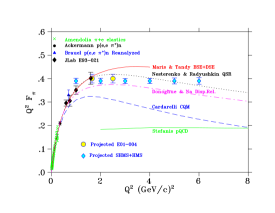
Figure 1: Summary of experimental data and phenomenological predictions for the pion electromagnetic form factor, taken from [4]. Note that some of the points show projected errors for proposed experiments.

What is surprising is that VMD with only the lightest $m_{\rho}$ resonance appears to describe all the existing data, even up to scales of $Q^{2}\gtrsim 1\mathrm{GeV}^{2}$ where one might have hoped the perturbative QCD (pQCD) would provide accurate predictions. At very high momentum transfer, we expect the perturbative description will be correct as computed in [5, 6, 7]

$$F_{\pi}(Q^{2})=\frac{8\pi\alpha_{s}(Q^{2})f_{\pi}^{2}}{Q^{2}}\quad\mathrm{as}\quad Q^{2}\to\infty$$ (3)

While the data may indicate an onset of the correct scale dependence around 2 $\mathrm{GeV}^{2}$, the numerical value is 100% larger than the pQCD asymptotic prediction.

This situation presents many questions. At what scale does the form factor scale with $Q^{2}$ as predicted by pQCD? Even if we assume proper scaling, the numerical values do not agree with pQCD. How rapidly will the data approach the pQCD prediction and at what scale will pQCD finally agree with the data? These are questions which Lattice QCD calculations are ideally suited to address, provided we can get reliable results for momentum transfer on the order of a few to several $\mathrm{GeV}^{2}$.

Early lattice calculations validated the vector meson dominance hypothesis at low $Q^{2}$ [8, 9]. Recent lattice results [10, 11], including some of our own preliminary results [12], have somewhat extended the range of momentum transfer, up to 2 $\mathrm{GeV}^{2}$, and the results remain consistent with VMD and the experimental data.

2 LATTICE COMPUTATION OF $F_{\pi}(Q^{2})$

The electromagnetic form factor is obtained in lattice QCD simulations by placing a charged pion creation operator at Euclidean time $t_{i}$, a charged pion annihilation operator at $t_{f}$ and a vector current insertion at $t$ as shown in Fig. 2. A standard quark propagator calculation provides the two propagator lines that originate from $t_{i}$. The remaining quark propagator, originating from $t_{f}$ is obtained via the sequential source method: (1) completely specify the quantum numbers, including momentum $\vec{p}_{f}$, of the annihilation operator to be placed at $t_{f}$ and (2) contract the propagator from $t_{i}$ to $t_{f}$ to the annihilation operator and use that product as the source vector of a second, sequential propagator inversion. The resulting sequential propagator appears as the thick line in Fig. 2 extending from $t_{i}$ to $t$ via $t_{f}$. Given these two propagators, the diagram can be computed for all possible values of insertion position $t$ and source and insertion momenta, $\vec{p}_{i}$ and $\vec{q}$, consistent with overall momentum conservation: $\vec{q}=\vec{p}_{f}-\vec{p}_{i}$. Furthermore, with the same set of propagators, any current can be inserted at $t$ and any meson creation operator can be contracted at $t_{i}$. So, the diagram relevant to determining the form factor for the transition $\rho^{+}\to\gamma\pi^{+}$ can be computed without further quark propagator calculations. By applying the sequential source method at the sink, the trade-off is that the entire set of sequential propagators must be recomputed each time new quantum numbers are needed at the sink, particularly $\vec{p}_{f}$.

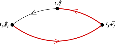
Figure 2: The quark propagators used to compute the pion form factor.

We can extract the pion energies $E_{\pi}(\vec{p})$ using standard lattice techniques of fitting pion correlation functions from which we can compute the momentum transfer

$$-Q^{2}=\left[E_{\pi}(\vec{p}_{f})-E_{\pi}(\vec{p}_{i})\right]^{2}-(\vec{p}_{f}-\vec{p}_{i})^{2}$$ (4)

which should be non-positive if the pion spectral function is well-behaved. Since the largest $Q^{2}$ occur in the Breit frame, $\vec{p}_{f}=-\vec{p}_{i}$, it is important to choose a non-zero $\vec{p}_{f}$ to achieve large momentum transfer.

The form factor, $F(Q^{2})$, is defined by

$$\left\langle\pi(\vec{p}_{f})\left|V_{\mu}(0)\right|\pi(\vec{p}_{i})\right\rangle_{\mathrm{continuum}}=$$

$$Z_{V}\left\langle\pi(\vec{p}_{f})\left|V_{\mu}(0)\right|\pi(\vec{p}_{i})\right\rangle=F(Q^{2})(p_{i}+p_{f})_{\mu}$$

where $V_{\mu}(x)$ is the chosen vector current. The three-point correlation function depicted in Fig. 2 is given by

$$\Gamma_{\pi\mu\pi}^{AB}(t_{i},t,t_{f},\vec{p}_{i},\vec{p}_{f})=$$

$$a^{9}\sum_{\vec{x}_{i},\vec{x}_{f}}e^{-i(\vec{x}_{f}-\vec{x})\cdot\vec{p}_{f}}\ \times\ e^{-i(\vec{x}-\vec{x}_{i})\cdot\vec{p}_{i}}$$

$$\quad\times\left\langle 0\left|\phi_{B}(x_{f})V_{\mu}(x)\phi_{A}^{\dagger}(x_{i})\right|0\right\rangle$$

where $\phi_{A}^{\dagger}(x)$ and $\phi_{B}(x)$ are creation and annihilation operators with pion quantum numbers. The $A$ and $B$ indicate that different operators may be used at the source and sink, i.e. smeared source and point sink or pseudoscalar source and axial vector sink.

Inserting complete sets of hadron states and requiring $t_{i}\ll t\ll t_{f}$, gives

$$\Gamma_{\pi\mu\pi}^{AB}(t_{i},t,t_{f},\vec{p}_{i},\vec{p}_{f})\to$$

$$a^{3}\left\langle 0\left|\phi_{B}(x)\right|\pi(\vec{p}_{f})\right\rangle\frac{e^{-(t_{f}-t)E_{\pi}(\vec{p}_{f})}}{2E_{\pi}(\vec{p}_{f})}$$

$$\times\left\langle\pi(\vec{p}_{f})\left|V_{\mu}(x)\right|\pi(\vec{p}_{i})\right\rangle$$

$$\times\frac{e^{-(t-t_{i})E_{\pi}(\vec{p}_{i})}}{2E_{\pi}(\vec{p}_{i})}\left\langle\pi(\vec{p}_{i})\left|\phi_{A}^{\dagger}(x)\right|0\right\rangle$$

Similarly for the two-point correlator and $t_{i}\ll t_{f}$

$$\Gamma_{\pi\pi}^{AB}(t_{i},t_{f},\vec{p})\to a^{3}\left\langle 0\left|\phi_{B}(x_{f})\right|\pi(\vec{p})\right\rangle$$

$$\times\frac{e^{-(t_{f}-t_{i})E_{\pi}(\vec{p})}}{2E_{\pi}(\vec{p})}\left\langle\pi(\vec{p})\left|\phi_{A}^{\dagger}(x_{i})\right|0\right\rangle$$

For pion operators, we use either the pseudoscalar density, $\phi^{(1)}(x)=\overline{\psi}(x)\gamma_{5}\psi(x)$, or the temporal component of the axial vector current, $\phi^{(2)}(x)=\overline{\psi}(x)\gamma_{5}\gamma_{4}\psi(x)$, at a single point, denoted “L” for local, or smeared, denoted “S,” using gauge invariant Gaussian smearing

$$b(x)\to\left(1+\frac{\omega}{N}\vec{\nabla}U\right)^{N}b(x).$$ (9)

Note that we have suppressed the flavor structure. For these operators, we get the following amplitudes

$$a^{2}\left\langle 0\left|\phi_{L}^{(1)}(x)\right|\pi(\vec{p})\right\rangle = Z_{L}^{(1)}e^{i\vec{x}\cdot\vec{p}}$$ (10)

$$a^{2}\left\langle 0\left|\phi_{S}^{(1)}(x)\right|\pi(\vec{p})\right\rangle = Z_{S}^{(1)}(\left|\vec{p}\right|)e^{i\vec{x}\cdot\vec{p}}$$ (11)

$$a^{2}\left\langle 0\left|\phi_{L}^{(2)}(x)\right|\pi(\vec{p})\right\rangle = Z_{L}^{(2)}(\left|\vec{p}\right|)e^{i\vec{x}\cdot\vec{p}}$$ (12)

$$a^{2}\left\langle 0\left|\phi_{S}^{(2)}(x)\right|\pi(\vec{p})\right\rangle = Z_{S}^{(2)}(\left|\vec{p}\right|)e^{i\vec{x}\cdot\vec{p}}$$ (13)

We anticipate that $Z_{L}^{(2)}(\vec{p})\propto E_{\pi}(\vec{p})$ based on the Lorentz structure of the operator. All of the $Z$’s should have corrections of $\mathcal{O}(p^{2})$.

From this discussion, we can see that there are two ways to determine the form factor $F_{\pi}(Q^{2})$. The first method, which we will call the fitting method involves a fit of the relevant two and three-point functions to simultaneously extract the form factor, the energies $E_{\pi}(\vec{p})$ and the amplitudes $Z(\vec{p})$ in a single covariant, jackknifed fit.

Another method, which we will call the ratio method starts by determining the energies $E_{\pi}(\vec{p})$ and then constructing the following ratio which is independent of $Z_{L}^{(1)}$, $Z_{S}(|\vec{p}|)$ and all Euclidean time exponentials:

$$F(Q^{2},t) = \frac{\Gamma_{\pi 4\pi}^{AB}(t_{i},t,t_{f},\vec{p}_{i},\vec{p}_{f})\Gamma_{\pi\pi}^{CL}(t_{i},t,\vec{p}_{f})}{\Gamma_{\pi\pi}^{AL}(t_{i},t,\vec{p}_{i})\Gamma_{\pi\pi}^{CB}(t_{i},t_{f},\vec{p}_{f})}$$ (14)

$$\times\left(\frac{2Z_{V}E_{\pi}(\vec{p}_{f})}{E_{\pi}(\vec{p}_{i}+E_{\pi}(\vec{p}_{f})}\right)$$

where the indices $A$, $B$ and $C$ can be either $L$ (local) or $S$ (smeared). For a conserved current, $Z_{V}\equiv 1$. As part of our program, we expect to determine the relative merits of each extraction method.

3 SIMULATION DETAILS

Table 1: Simulation details for quenched Wilson fermion calculations at $a^{-1}\approx 2\ \mathrm{GeV}$

. $\kappa$ volume $am_{\pi}$ $am_{\rho}$ 0.1480 $16^{3}\times 32$ 0.673 0.712 0.1520 $16^{3}\times 32$ 0.477 0.549 0.1540 $16^{3}\times 32$ 0.364 0.468 0.1555 $24^{3}\times 32$ 0.259 0.398 0.1563 $24^{3}\times 32$ 0.179 0.358 0.1566 $24^{3}\times 32$ 0.145 0.343 0.1566 $32^{3}\times 48$ 0.145 0.343

Our first calculations were done on quenched configurations generated with the Wilson gauge action at $\beta=6.0$ ($a^{-1}\approx 2\ \mathrm{GeV}$). The propagators were computed using the unimproved Wilson fermion action with Dirichlet boundary conditions. For Wilson fermions at these lattice spacings, the exceptional configuration problem is rather mild particularly when compared to non-perturbatively improved Clover action. This enabled us to reach pion masses of 300 MeV without observing any exceptional configurations, see Tab. 1 whereas Clover simulations are limited to pions of roughly 500 MeV [10]. Of course, pion masses in quenched domain wall fermion calculations are limited only by finite volume effects and available computing power. Yet the best results so far for pion form factors are 390 MeV pions at $a^{-1}\approx 1.3\ \mathrm{GeV}$ lattice spacing [11]. Furthermore, at this workshop we learned that Wilson fermion results may be automatically $\mathcal{O}(a)$ improved with just double the effort [13], which is an option we have under consideration for the future.

Table 2: Simulation details for domain wall fermion calculations on 272 dynamical MILC asqtad lattices at $a^{-1}\approx 1.5\ \mathrm{GeV}$.

$am_{u,d}$	$am_{s}$	$am_{\mathrm{dwf}}$	Volume	$am_{\pi}$
0.01	0.05	0.01	$20^{3}\times 64$	0.200

For our unquenched results, we used valence domain wall fermions with a domain wall height of $m_{0}=1.7$ and $L_{s}=16$ on MILC $N_{f}=2+1$ and $N_{f}=3$ lattices after HYP blocking [14]. Dirichlet boundary conditions were imposed 32 timeslices apart for the domain wall propagator calculations. Detailed results of several quantities computed on these MILC configurations were presented at this workshop [15]. Preliminary results on related hadronic observables using many of the same domain wall propagators have recently been presented [16] and were also discussed at this workshop.

4 PRELIMINARY RESULTS

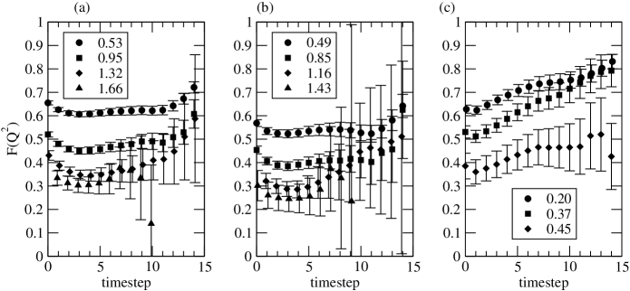
Figure 3: Pion form factor data versus timestep, for (a) $\kappa$=0.1520, (b) $\kappa$=0.1540 and (c) $\kappa$=0.1563. Numerical values of $Q^{2}$ in GeV are shown in the legends.

Representative plots of the pion form factor and it’s dependence on the timeslice of the current insertion $F_{\pi}(Q^{2},t)$ are shown in Fig. 3. The form factors in these plots were computed using the ratio method. For the heavier pion masses (smaller values of $\kappa$) there are nice plateaus which indicate reasonable signal to noise for all momenta considered and little contamination from excited states. As the pion masses get lighter, the signal to noise decreases and the plateaus become less convincing which suggest that the source and sink may not be sufficiently separated and hence excited states may be contaminating the ratio. Another possibility is that the ratio may not provide an optimal determination of the form factor at lighter pion masses. A detailed study is currently in progress.

Preliminary results of the quenched Wilson form factor computed by the fitting method are plotted in Fig. 4. Also shown in the figure are experimental data points and a curve showing the prediction of vector meson dominance using the observed value for the $\rho$ meson mass. While the data tend in the correct direction with decreasing pion mass, the reader may notice that the form factor for 300 MeV pions already lies below the physical curve. This suggests that fitting the data to extract a lattice determination of the vector meson mass would underestimate the physical value. In fact, this is exactly what one should expect since it is known that $\mathcal{O}(a)$ scaling violations to the vector meson mass computed with Wilson fermions tend to underestimate the mass by roughly 20% [17], the same amount needed to move the form factor points above the continuum curve. Hence, the proposal of Frezzotti and Rossi [13] becomes all the more appealing as a straightforward way to remove what is presumably an $\mathcal{O}(a)$ lattice artifact.

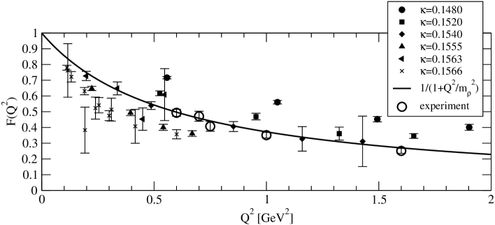
Figure 4: Results for the pion form factor as a function of $Q^{2}$ for each of the available $\kappa$ values. Experimental measurements[18] and the vector meson dominance hypothesis are also shown.

Because we would like to compute the pion form factor at large momentum transfer, we have spent a substantial amount of effort on our domain wall data set in extracting the pion energies and amplitudes at relatively large momenta. In the continuum limit, the pion dispersion relation should follow the continuum one

$$E_{\pi}(\vec{p})^{2}=\vec{p}^{2}+E_{\pi}(0)^{2}$$ (15)

Another possibility is that the pion dispersion relation will follow the dispersion relation of a free lattice boson

$$\frac{1}{4}\sinh^{2}\left(\frac{E_{\pi}(\vec{p})}{2}\right)=$$

$$\frac{1}{4}\sin^{2}\left(\frac{\vec{p}}{2}\right)+\frac{1}{4}\sinh^{2}\left(\frac{E_{\pi}(0)}{2}\right)$$

Both relations agree in the small momentum limit.

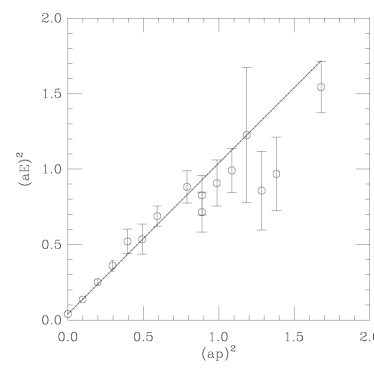
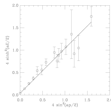
Figure 5: Pion dispersion relation vs. continuum (left) and lattice (right) expectations.

In Fig. 5, we have plotted against each dispersion relation and we see that both dispersion relations provide a reasonable representation of the data, although there may be a slight flattening of the data against the continuum curve at higher momenta. These results suggest that directly fitting all the data to either dispersion relation, thereby reducing the number of fit parameters needed to extract the form factor, may improve the relative signal to noise of the remaining parameters. This may help dramatically in the ratio method, where the only fit parameters are the form factor and the energies.

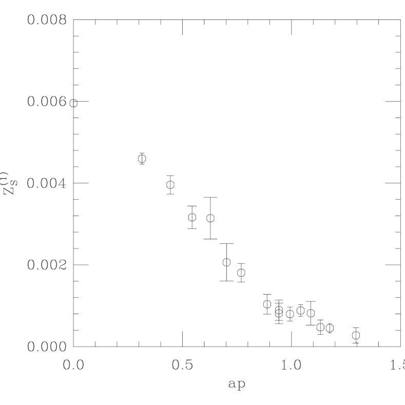
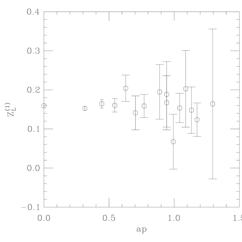
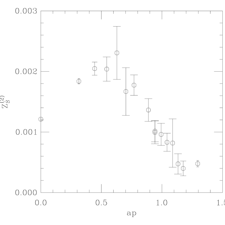
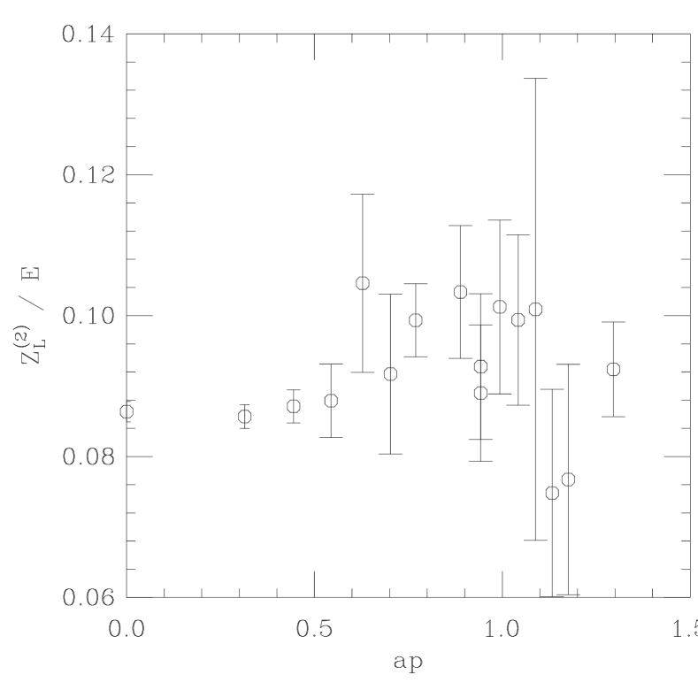
Figure 6: Results for the four pion source amplitudes $Z_{A}^{(i)}(\vec{p})$ used in this study.

In the fitting method, one must reliably estimate not only the energies, but the amplitudes, at high momenta. In Fig. 6 we present the four amplitudes we estimate from the four two-point correlators we measure: smeared-smeared and smeared-local for both pseudoscalar-pseudoscalar and axial-axial operators. In the fitting procedure, all four correlators are constrained to have the same energy. From the figure, we can see that our expectations of $Z_{L}^{(1)}\propto\mathrm{const}$ and $Z_{L}^{(2)}(\vec{p})\propto E_{\pi}(\vec{p})$ are consistent with the data. We can also see from $Z_{S}^{(1)}$ that the smeared pseudoscalar operator has a strong overlap with the zero momentum pion but that the overlap diminishes rapidly with increasing momenta. From $Z_{S}^{(2)}$ we see that the smeared axial-vector operator has good overlap over a wide range of non-zero momenta, with maximal overlap around $ap\sim 0.5$. Thus, given the variety of sources and their relative strengths of overlapping with pions at different momenta was key to fitting pion energies up to such high momenta.

5 CONCLUSIONS

From our preliminary quenched Wilson form factor results, we find that both the ratio method and the fitting method are useful tools for computing the pion form factor. Each method has different systematic errors, so the extent to which both agree should give confidence that the systematic errors are small and well understood.

From our preliminary dynamical domain wall spectrum results, we recognize the importance of using a large basis of pion operators so that at least one will have reasonable overlap with the momenta under consideration. The local axial vector operator is particularly useful in fitting higher momentum states since it’s overlap with a given state increases as the energy increases.

In the near future, when the pion form factor analysis is complete, it will be a straightforward extension to our existing analysis framework to compute the $\rho^{+}\to\gamma\pi^{+}$ transition form factors using the propagators and sequential propagators we have already computed.

References

- [1] W.G. Holladay, Phys. Rev. 101 (1956) 1198.
- [2] W.R. Frazer and J.R. Fulco, Phys. Rev. Lett. 2 (1959) 365.
- [3] W.R. Frazer and J.R. Fulco, Phys. Rev. 117 (1960) 1609.
- [4] H.P. Blok, G.M. Huber and D.J. Mack, (2002), nucl-ex/0208011.
- [5] S.J. Brodsky and G.R. Farrar, Phys. Rev. Lett. 31 (1973) 1153.
- [6] S.J. Brodsky and G.R. Farrar, Phys. Rev. D11 (1975) 1309.
- [7] G.R. Farrar and D.R. Jackson, Phys. Rev. Lett. 43 (1979) 246.
- [8] G. Martinelli and C.T. Sachrajda, Nucl. Phys. B306 (1988) 865.
- [9] T. Draper et al., Nucl. Phys. B318 (1989) 319.
- [10] J. van der Heide et al., Phys. Lett. B566 (2003) 131, hep-lat/0303006.
- [11] RBC, Y. Nemoto, (2003), hep-lat/0309173.
- [12] LHPC, F.D.R. Bonnet et al., (2003), hep-lat/0310053.
- [13] R. Frezzotti and G.C. Rossi, (2003), hep-lat/0311008.
- [14] A. Hasenfratz and F. Knechtli, Phys. Rev. D64 (2001) 034504, hep-lat/0103029.
- [15] S. Gottlieb, (2003), hep-lat/0310041.
- [16] LHPC, W. Schroers et al., (2003), hep-lat/0309065.
- [17] R.G. Edwards, U.M. Heller and T.R. Klassen, Phys. Rev. Lett. 80 (1998) 3448, hep-lat/9711052.
- [18] The Jefferson Lab F(pi), J. Volmer et al., Phys. Rev. Lett. 86 (2001) 1713, nucl-ex/0010009.