Numerical Methods for the QCD Overlap Operator: II. Optimal Krylov Subspace Methods

Abstract

We investigate optimal choices for the (outer) iteration method to use when solving linear systems with Neuberger’s overlap operator in QCD. Different formulations for this operator give rise to different iterative solvers, which are optimal for the respective formulation. We compare these methods in theory and practice to find the overall optimal one. For the first time, we apply the so-called SUMR method of Jagels and Reichel to the shifted unitary version of Neuberger’s operator, and show that this method is in a sense the optimal choice for propagator computations. When solving the “squared” equations in a dynamical simulation with two degenerate flavours, it turns out that the CG method should be used.

1 Introduction

Recently, lattice formulations of QCD respecting chiral symmetry have attracted a lot of attention. A particular promising such formulation, the so-called overlap fermions, has been proposed in Narayanan:2000qx . From the computational point of view, we have to solve linear systems involving the sign function $\hbox{\rm\,sign}(Q)$ of the (hermitian) Wilson fermion matrix $Q$. These computations are very costly, and it is of vital importance to devise efficient numerical schemes.

A direct computation of $\hbox{\rm\,sign}(Q)$ is not feasible, since $Q$ is large and sparse, whereas $\hbox{\rm\,sign}(Q)$ would be full. Therefore, numerical algorithms have to follow an inner-outer paradigm: One performs an outer Krylov subspace method where each iteration requires the computation of a matrix-vector product involving $\hbox{\rm\,sign}(Q)$. Each such product is computed through another, inner iteration using matrix-vector multiplications with $Q$. In an earlier paper EFL02 we investigated methods for the inner iteration and established the Zolotarev rational approximation together with the multishift CG method Glassner:1996gz as the method of choice.

In the present paper we investigate optimal methods for the outer iteration. We consider two situations: the case of a propagator computation and the case of a pseudofermion computation within a dynamical hybrid Monte Carlo simulation where one has to solve the “squared” system. As we will see, the optimal method for the case of a propagator computation is a not so well-known method due to Jagels and Reichel JR94 , whereas in the case of the squared system it will be best to apply classical CG on that squared system rather than using a two-pass approach.

This paper is organized as follows: We first introduce our notation in Section 2. We then discuss different equivalent formulations of the Neuberger overlap operator and establish useful relations between the eigenpairs of these different formulations (Section 3). We discuss optimal Krylov subspace methods for the various systems in Section 4 and give some theoretical results on their convergence speed based on the spectral information from Section 3. In Section 5 we compare the convergence speeds both, theoretically and in practical experiments. Our conclusions will be summarized in Section 6.

2 Notation

The Wilson-Dirac fermion operator,

$$M=I-\kappa D_{W},$$ (1)

represents a nearest neighbour coupling on a four-dimensional space-time lattice, where the “hopping term” $D_{W}$ is a non-normal sparse matrix, see (25) in the appendix. The coupling parameter $\kappa$ is a real number which is related to the bare quark mass.

The massless overlap operator is defined as

$$D_{0}=I+M\cdot(M^{\dagger}M)^{-\frac{1}{2}}.$$

For the massive overlap operator, for notational convenience we use a mass parameter $\rho>1$ such that this operator is given as

$$D=\rho I+M\cdot(M^{\dagger}M)^{-\frac{1}{2}}.$$ (2)

In the appendix, we explain that this form is just a scaled version of Neuberger’s original choice, and we relate $\rho$ to the quark mass, see (29) and (30).

Replacing $M$ in (2) by its hermitian form $Q$, see (26), the overlap operator can equivalently be written as

$$D=\rho I+\gamma_{5}\hbox{\rm\,sign}(Q)=\gamma_{5}\cdot(\rho\gamma_{5}+\hbox{\rm\,sign}(Q)),$$ (3)

with $\gamma_{5}$ being defined in (27) and $\hbox{\rm\,sign}(Q)$ being the standard matrix sign function. Note that $\rho\gamma_{5}+\hbox{\rm\,sign}(Q)$ is hermitian and indefinite, whereas $\gamma_{5}\hbox{\rm\,sign}(Q)$ is unitary.

To reflect these facts in our notation, we define:

$$D_{u}=\rho I+\gamma_{5}\hbox{\rm\,sign}(Q),\qquad D_{h}=\rho\gamma_{5}+\hbox{\rm\,sign}(Q),$$

where $D_{u}=\gamma_{5}D_{h}$. Both these operators are normal, i.e. they commute with their adjoints.

3 Formulations and their spectral properties

3.1 Propagator computations

When computing quark propagators, the systems to solve are of the form

$$D_{u}x=(\rho I+\gamma_{5}\hbox{\rm\,sign}(Q))x=b.$$ (4)

Multiplying this shifted unitary form by $\gamma_{5}$, we obtain its hermitian indefinite form as

$$D_{h}x=(\rho\gamma_{5}+\hbox{\rm\,sign}(Q))x=\gamma_{5}b.$$ (5)

The two operators $D_{u}$ and $D_{h}$ are intimately related. They are both normal, and as a consequence the eigenvalues (and the weight with which the corresponding eigenvectors appear in the initial residual) solely govern the convergence behaviour of an optimal Krylov subspace method used to solve the respective equation.

Very interestingly, the eigenvalues of the different operators can be explicitly related to each other. This allows a quite detailed discussion of the convergence properties of adequate Krylov subspace solvers. To see this, let us introduce an auxiliary decomposition for $\hbox{\rm\,sign}(Q)$: Using the chiral representation, the matrix $\gamma_{5}$ on the whole lattice can be represented as a $2\times 2$ block diagonal matrix

$$\gamma_{5}=\left(\begin{array}[]{cc}I&0\\ 0&-I\end{array}\right),$$ (6)

where both diagonal blocks $I$ and $-I$ are of the same size. Partitioning $\hbox{\rm\,sign}(Q)$ correspondingly gives

$$\hbox{\rm\,sign}(Q)=\left(\begin{array}[]{cc}S_{11}&S_{12}\\ S^{\dagger}_{12}&S_{22}\end{array}\right).$$ (7)

In Lemma 1 below we give a convenient decomposition for this matrix that is closely related to the so-called CS decomposition (see (GLo96, , Theorem 2.6.3) and the references therein), an important tool in matrix analysis. Actually, the lemma may be regarded as a variant of the CS decomposition for hermitian matrices where the decomposition here can be achieved using a similarity transform. The proof follows the same lines as the proof for the existence of the CS decomposition given in PWe94 .

Lemma 1

There exists a unitary matrix $X$ such that

$$\hbox{\rm\,sign}(Q)=X\left(\begin{array}[]{cc}\Phi&\Sigma\\ \Sigma&\Psi\end{array}\right)X^{\dagger},\quad\hbox{ with }X=\left(\begin{array}[]{cc}X_{1}&0\\ 0&X_{2}\end{array}\right).$$

The matrices $\Phi$, $\Psi$ and $\Sigma$ are real and diagonal with diagonal elements $\phi_{j}$, $\psi_{j}$ and $\sigma_{j}\geq 0$, respectively. Furthermore, $\phi_{j}^{2}+\sigma_{j}^{2}=\psi_{j}^{2}+\sigma_{j}^{2}=1$ and

$$\phi_{j}=-\psi_{j}\quad \hbox{if}\quad\sigma_{j}>0$$ (8)

$$\phi_{j},\psi_{j}\in\{-1,+1\}\quad \hbox{if}\quad\sigma_{j}=0.$$ (9)

Note that in the case of (8) we know that $\phi_{j}$ and $\psi_{j}$ have opposite signs, whereas in case (9) we might have $\phi_{j}=\psi_{j}=1$ or $\phi_{j}=\psi_{j}=-1$. The key point for $X$ in Lemma 1 is the fact that $\gamma_{5}X=X\gamma_{5}$. This allows us to relate the eigenvalues and -vectors of the different formulations for the overlap operator via $\phi_{j}$, $\psi_{j}$ and $\sigma_{j}$. In this manner we give results complementary to Edwards et al. EHN98 , where relations between the eigenvalues (and partly the -vectors) of the different formulations for the overlap operator were given without connecting them to $\hbox{\rm\,sign}(Q)$ via $\phi_{j}$, $\psi_{j}$ and $\sigma_{j}$. The following lemma gives expressions for the eigenvectors and -values of the shifted unitary operator $D_{u}$.

Lemma 2

With the notation from Lemma 1, let $x_{j}^{1}$ and $x_{j}^{2}$ be the $j$-th column of $X_{1}$ and $X_{2}$, respectively. Then $\mbox{{\rm spec}}(D_{u})=\{\lambda_{j,\pm}^{u}\}$ with

$$\lambda_{j,\pm}^{u}=\rho+\phi_{j}\pm i\sqrt{1-\phi^{2}_{j}} \quad\mbox{ if }\quad\sigma_{j}\not=0$$

$$\lambda_{j,+}^{u}=\rho+\phi_{j},\;\lambda_{j,-}^{u}=\rho-\psi_{j} \quad\mbox{ if }\quad\sigma_{j}=0.$$

The corresponding eigenvectors are

$$\begin{array}[]{ll}z^{u}_{j,\pm}=\left(\begin{array}[]{c}\mp ix_{j}^{1}\\ x_{j}^{2}\end{array}\right)&\quad\mbox{ if }\quad\sigma_{j}\not=0\\ z^{u}_{j,+}=\left(\begin{array}[]{c}x_{j}^{1}\\ 0\end{array}\right),\;z^{u}_{j,-}=\left(\begin{array}[]{c}0\\ x_{j}^{2}\end{array}\right)&\quad\mbox{ if }\quad\sigma_{j}=0.\end{array}$$ (10)

Proof

With the decomposition for $\hbox{\rm\,sign}(Q)$ in Lemma 1, we find, using $X^{\dagger}\gamma_{5}=\gamma_{5}X^{\dagger}$,

$$X^{\dagger}\gamma_{5}\hbox{\rm\,sign}(Q)X=\gamma_{5}X^{\dagger}\hbox{\rm\,sign}(Q)X\\ =\left(\begin{array}[]{cc}\Phi&\Sigma\\ -\Sigma&-\Psi\end{array}\right).$$

Since the actions of $X$ and $X^{\dagger}$ represent a similarity transform, we can easily derive the eigenvalues and eigenvectors of $\gamma_{5}\hbox{\rm\,sign}(Q)$ from the matrix on the right. This can be accomplished by noticing that this matrix can be permuted to have a block diagonal form with $2\times 2$ blocks on the diagonal, so that the problem reduces to the straightforward computation of the eigenvalues and eigenvectors of $2\times 2$ matrices. This concludes the proof.

As a side remark, we mention that Edwards et al. EHN98 observed that the eigenvalues of $D_{u}$ can be efficiently computed by exploiting the fact that most of the eigenvalues come in complex conjugate pairs. Indeed, using Lemma 1 and the fact that $\gamma_{5}X=X\gamma_{5}$ we see that we only have to compute the eigenvalues of the hermitian matrix $S_{11}$ (and to check for one or minus one eigenvalues in $S_{22}$).

With the same technique as in Lemma 2 we can also find expressions for the eigenvalues and eigenvectors of the hermitian indefinite formulation.

Lemma 3

With the same notation as in Lemma 2, we have that $\mbox{{\rm spec}}(D_{h})=\{\lambda^{h}_{j,\pm}\}$ with

$$\lambda^{h}_{j,\pm}=\pm\sqrt{1+2\phi_{j}\rho+\rho^{2}} \quad\mbox{ if }\quad\sigma_{j}\not=0$$

$$\lambda^{h}_{j,+}=\rho+\phi_{j},\;\lambda^{h}_{j,-}=-\rho+\psi_{j} \quad\mbox{ if }\quad\sigma_{j}=0.$$

The corresponding eigenvectors are

$$z^{h}_{j,\pm}=\left(\begin{array}[]{c}(\phi_{j}\rho+\lambda_{j,\pm}^{h})x_{j}^{1}\\ \sqrt{1-\phi_{j}^{2}}\,x_{j}^{2}\end{array}\right)\; \quad\mbox{ if }\quad\sigma_{j}\not=0,$$

$$z^{h}_{j,+}=\left(\begin{array}[]{c}x_{j}^{1}\\ 0\end{array}\right),\;z^{h}_{j,-}=\left(\begin{array}[]{c}0\\ x_{j}^{2}\end{array}\right)\; \quad\mbox{ if }\quad\sigma_{j}=0.$$

As an illustration to the results of this section, we performed numerical computations for two sample configurations. Both are on a $4^{4}$ lattice with $\beta=6.0$ (configuration A) and $\beta=5.0$ (configuration B) respectively. Figure 1 shows plots of the eigenvalues of $M$ for these configurations. We used $\kappa=0.2129$ for configuration A, $\kappa=0.2809$ for configuration B.

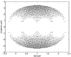
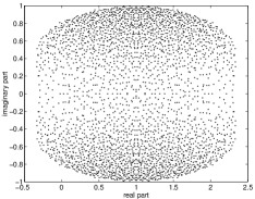
Figure 1: Eigenvalues for the Wilson fermion matrix $M$ for configurations A (left) and B (right)

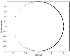
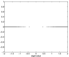
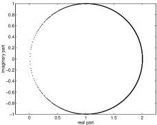
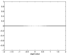
Figure 2: Eigenvalues of $D_{u}$ (left column) and $D_{h}$ (right column) all for $\rho=1.01$. The upper plots are for configuration A, the lower for configuration B.

Figure 2 gives plots of the eigenvalues of $D_{u}$ and $D_{h}$ for our example configurations with $\rho=1.01$. It illustrates some interesting consequences of Lemma 2 and Lemma 3: With $C(\rho,1)$ denoting the circle in the complex plane with radius 1 centered at $\rho$, we have

$$\mbox{{\rm spec}}(D_{u})\subseteq C(\rho,1),$$ (13)

and, moreover, $\mbox{{\rm spec}}(D_{u})$ is symmetric w.r.t. the real axis. On the other hand, $\mbox{{\rm spec}}(D_{h})$ is “almost symmetric” w.r.t. the origin, the only exceptions corresponding to the case $\sigma_{j}$ = 0, where an eigenvalue of the form $\rho+\phi_{j}$ with $\phi_{j}\in\{\pm 1\}$ not necessarily matches $-\rho+\psi_{j}$ with $\psi_{j}\in\{\pm 1\}$, since we do not necessarily have $\psi_{j}=-\phi_{j}$. Moreover,

$$\mbox{{\rm spec}}(D_{h})\subseteq[-(\rho+1),-(\rho-1)]\cup[(\rho-1),(\rho+1)].$$ (14)

Finally, let us note that we have some $\sigma_{j}$ equal to zero as soon as 0 is an eigenvalue of the massless operator $\gamma_{5}+\hbox{\rm\,sign}(Q)$, i.e., as soon as the configuration has non-trivial topology.

3.2 Dynamical simulations

In a simulation with dynamical fermions, the costly computational task is the inclusion of the fermionic part of the action into the “force” evolving the gauge fields. This requires to solve the “squared” system

$$D_{u}^{\dagger}D_{u}x=b\;\Longleftrightarrow\;D_{h}^{2}x=b.$$

We will denote $D_{n}$ the respective operator, i.e.,

$$D_{n}=D_{h}^{2}=D_{u}^{\dagger}D_{u}.$$

If we plug in the definition of $D_{u}$, we find that

$$D_{n}y=D_{u}^{\dagger}D_{u}y=\left((\rho^{2}+1)I+\rho(\gamma_{5}\hbox{\rm\,sign}(Q)+\hbox{\rm\,sign}(Q)\gamma_{5})\right)y=b,$$ (15)

from which we get the interesting relation

$$D_{u}D_{u}^{\dagger}=\gamma_{5}D_{u}^{\dagger}D_{u}\gamma_{5}=D_{u}^{\dagger}D_{u}.$$ (16)

As is well known, (15) becomes block diagonal, since, using (6) and (7), we have

$$D_{n}=\left(\begin{array}[]{cc}(\rho^{2}+1)I+2\rho S_{11}&0\\ 0&(\rho^{2}+1)I-2\rho S_{22}\end{array}\right)y=b.$$ (17)

In practical simulations, the decoupled structure of (17) can be exploited by running two seperate CG processes simultaneously, one for each (half-size) block. Since each of these CG processes only has to accomodate a part of the spectrum of $D_{n}$, convergence will be faster. An alternative usage of the block structure is to compute the action of the matrix sign function on a two-dimensional subspace corrresponding to the two blocks and to use a block type Krylov subspace method. We do not, however, pursue this aspect further, here. As another observation, let us note that if $\gamma_{5}b=\pm b$, then computing $D_{n}b$ requires only one evaluation of the sign function instead of two (“chiral projection approach”).

As with the other formulations, let us summarize the important spectral properties of the squared operator $D_{n}$.

Lemma 4

With the notation of Lemma 1, $\mbox{{\rm spec}}(D_{n})=\{\lambda_{j,\pm}^{n}\}$ with

$$\lambda^{n}_{j,\pm}=1+2\phi_{j}\rho+\rho^{2}\enspace\mbox{(double eigenvalue) } \quad\mbox{ if }\quad\sigma_{j}\not=0$$

$$\lambda_{j,+}=(\rho+\phi_{j})^{2},\;\lambda_{j,-}=(-\rho+\psi_{j})^{2} \quad\mbox{ if }\quad\sigma_{j}=0.$$

The corresponding eigenvectors are the same as for $D_{h}$ or, equivalently, the same as for $D_{u}$ or, again equivalently,

$$\left(\begin{array}[]{c}x^{1}_{j}\\ 0\end{array}\right),\;\left(\begin{array}[]{c}0\\ x^{2}_{j}\end{array}\right)\;.$$

Notice also that $\mbox{{\rm spec}}(D_{n})$ satisfies

$$\mbox{{\rm spec}}(D_{n})\subseteq[(\rho-1)^{2},(\rho+1)^{2}].$$ (18)

4 Optimal Krylov subspace methods

4.1 Propagator computation

Let us start with the non-hermitian matrix $D_{u}$. Due to its shifted unitary form, there exists an optimal Krylov subspace method based on short recurrences to solve (4). This method was published in JR94 and we would like to term it SUMR (shifted unitary minimal residual). SUMR is mathematically equivalent to full GMRES, so its residuals $r^{m}=b-D_{u}x^{m}$ at iteration $m$ are minimal in the 2-norm in the corresponding affine Krylov subspace $x^{0}+K_{m}(D_{u},r^{0})$ where $K_{m}(D_{u},r^{0})=\mbox{{\rm span}}\{r^{0},D_{u}r^{0},\ldots,D_{u}^{m-1}r^{0}\}$. From the algorithmic point of view, SUMR is superior to full GMRES, since it relies on short recurrences and therefore requires constant storage and an equal amount of arithmetic work (one matrix vector multiplication and some vector operations) per iteration. The basic idea of SUMR is the observation that the upper Hessenberg matrix which describes the recursions of the Arnoldi process is shifted unitary so that its representation as a product of Givens rotations can be updated easily and with short recurrences. For the full algorithmic description we refer to JR94 .

Based on the spectral properties of $D_{u}$ that we identified in Section 3, we can derive the following result on the convergence of SUMR for (4).

Lemma 5

Let $x^{k}$ be the $k$-th iterate of SUMR applied to (4) and let $r_{u}^{k}$ be its residual. Then the following estimate holds:

$$\|r_{u}^{k}\|_{2}\leq 2\cdot\left(\frac{1}{\rho}\right)^{k}\|r_{u}^{0}\|_{2}.$$ (19)

Proof

Since $D_{u}$ is normal, its field of values $F(D_{u})=\{\langle D_{u}x,x\rangle,\|x\|_{2}=1\}$ is the convex hull of its eigenvalues so that we have $F(D_{u})\subseteq C(\rho,1)$, the disk centered at $\rho$ with radius 1. A standard result for full GMRES (which is mathematically equivalent to SUMR) now gives (19), see, e.g., Gre97 .

Let us proceed with the hermitian operator $D_{h}$ from (5), which is highly indefinite. The MINRES method is the Krylov subspace method of choice for such systems: It relies on short recurrences and it produces optimal iterates $x^{k}$ in the sense that their residuals $r^{k}_{h}=\gamma_{5}b-D_{h}x^{k}$ are minimal in the 2-norm over the affine subspace $x^{0}+K_{m}(D_{h},r^{0}_{h})$.

Lemma 6

Let $x^{k}$ be the iterate of MINRES applied to (5) at iteration $k$ and let $r_{h}^{k}$ be its residual. Then the following estimate holds:

$$\|r_{h}^{k}\|_{2}\leq 2\cdot\left(\frac{1}{\rho}\right)^{\lfloor k/2\rfloor}\|r_{h}^{0}\|_{2}.$$ (20)

Here, $\lfloor k/2\rfloor$ means $k/2$ rounded downwards to the nearest integer.

Proof

(20) is the standard MINRES estimate (see Gre97 ) with respect to the information from (14).

As a last approach to solving the propagator equation, let us consider the standard normal equation

$$D_{u}D_{u}^{\dagger}z=b,\;x=D_{u}^{\dagger}z.$$ (21)

Note that there exists an implementation of the CG method for (21) known as CGNE GLo96 which computes $x^{k}=D_{u}^{\dagger}z^{k}$ and its residual with respect to (4) on the fly, i.e., without additional work.

4.2 Dynamical simulations

We now turn to the squared equation (15). Since $D_{n}$ is hermitian and positive definite, the CG method is the method of choice for the solution of (15), its iterates $y^{m}$ achieving minimal error in the energy norm (see Lemma 7 below) over the affine Krylov subspace $y^{0}+K_{m}(D_{n},r^{0})$.

Lemma 7

Let $y^{k}$ be the iterate of CG applied to (15) at stage $k$. Then the following estimates hold ($y^{*}=D_{n}^{-1}b$)

$$\|y^{k}-y^{*}\|_{D_{n}} \leq 2\cdot\left(\frac{1}{\rho}\right)^{k}\|y^{0}-y^{*}\|_{D_{n}},$$ (22)

$$\|y^{k}-y^{*}\|_{2} \leq 2\cdot\frac{\rho+1}{\rho-1}\left(\frac{1}{\rho}\right)^{k}\|y^{0}-y^{*}\|_{2}.$$ (23)

Here, $\|\cdot\|_{D_{n}}$ denotes the energy norm $\|y\|_{D_{n}}=\sqrt{y^{\dagger}D_{n}y}$.

Proof

The energy norm estimate (22) is the standard estimate for the CG method based on the bound $\mbox{{\rm cond}}(D_{n})\leq\left((\rho+1)/(\rho-1)\right)^{2}$ for the condition number of $D_{n}$. The $2$-norm estimate follows from the energy norm estimate using

$$\|y\|_{2}\leq\sqrt{\|D_{n}^{-1}\|_{2}}\cdot\|y\|_{D_{n}}\leq\sqrt{\|D_{n}\|_{2}}\cdot\|y\|_{2}$$

with $\|D_{n}^{-1}\|_{2}\leq 1/(\rho-1)^{2},\;\|D_{n}\|_{2}\leq(\rho+1)^{2}$.

5 Comparison of methods

Based on Lemma 5 to 7 we now proceed by theoretically investigating the work for each of the three methods proposed so far. We consider two tasks: A propagator computation where we compute the solution $x$ from (4) or (5), and a dynamical simulation where we need to solve (15).

5.1 Propagator computation

The methods to be considered are SUMR for (4), MINRES for (5) and CGNE for (21). Note that due to (16), Lemma 7 can immediately also be applied to the CGNE iterates $z^{k}$ which approximate the solution $z$ of (21). In addition, expressing (22) in terms of $x^{k}=D^{\dagger}_{u}z^{k}$ instead of $z^{k}$ turns energy norms into 2-norms, i.e. we have

$$\|x^{k}-x^{*}\|_{2}\leq 2\cdot\left(\frac{1}{\rho}\right)^{k}\|x^{0}-x^{*}\|_{2}.$$ (24)

In order to produce a reasonably fair account of how many iterations we need, we fix a given accuracy $\varepsilon$ for the final error and calculate the first iteration $k(\varepsilon)$ for which the results given in Lemmas 5 and 6 and in (24) guarantee

$$\parallel x^{k(\varepsilon)}-x^{\ast}\parallel_{2}\,\leq\varepsilon\cdot\parallel r^{0}\parallel_{2},\quad x^{\ast}\mbox{ solution of (\ref{unitary_eq})},$$

where $r^{0}=b-D_{u}x^{0}$, $x^{0}$ being an identical starting vector for all three methods (most likely, $x^{0}=0$). Since $k(\varepsilon)$ will also depend on $\rho$, let us write $k(\varepsilon,\rho)$. The following may then be deduced from Lemma 5 and 6 and (24) in a straightforward manner.

Lemma 8

• For SUMR we have

  $$\parallel x^{k}-x^{\ast}\parallel_{2}\,\leq\frac{1}{\rho-1}\cdot\parallel r^{k}_{u}\parallel_{2}\,\leq\frac{2}{\rho-1}\left(\frac{1}{\rho}\right)^{k}\cdot\parallel r^{0}\parallel_{2},$$

  and therefore

  $$k(\varepsilon,\rho)\,\leq\frac{-\ln(\varepsilon)}{\ln(\rho)}+\frac{-\ln(2/(\rho-1))}{\ln(\rho)}.$$

• For MINRES we have using $\|r_{h}^{0}\|=\|r_{u}^{0}\|$, since $r_{h}^{0}=\gamma_{5}r_{u}^{0}$

  $$\parallel x^{k}-x^{\ast}\parallel_{2}\,\leq\frac{1}{\rho-1}\cdot\parallel r^{k}_{h}\parallel_{2}\,\leq\frac{2}{\rho-1}\cdot\left(\frac{1}{\rho}\right)^{\lfloor\frac{k}{2}\rfloor}\cdot\parallel r^{0}_{h}\parallel_{2},$$

  and therefore

  $$k(\varepsilon,\rho)\,\leq 2\cdot\left(\frac{-\ln(\varepsilon)}{\ln(\rho)}+\frac{-\ln(2/(\rho-1))}{\ln(\rho)}\right).$$

• For CGNE we have

  $$\parallel x^{k}-x^{\ast}\parallel_{2}\,\leq 2\cdot\left(\frac{1}{\rho}\right)^{k}\cdot\parallel x^{0}-x^{\ast}\parallel_{2}\,\leq 2\cdot\left(\frac{1}{\rho}\right)^{k}\cdot\frac{1}{\rho-1}\cdot\parallel r^{0}\parallel_{2},$$

  and therefore

  $$k(\varepsilon,\rho)\,\leq\frac{-\ln(\varepsilon)}{\ln(\rho)}+\frac{-\ln(2/(\rho-1))}{\ln(\rho)}.$$

The arithmetic work in all these iterative methods is completely dominated by the cost for evaluating the matrix vector product $\hbox{\rm\,sign}(Q)v$. MINRES and SUMR require one such evaluation per iteration, whereas CGNE requires two. Taking this into account, Lemma 8 suggests that MINRES and CGNE should require about the same work to achieve a given accuracy $\varepsilon$, whereas SUMR should need only half as much work, thus giving a preference for SUMR. Of course, such conclusions have to be taken very carefully: In a practical computation, the progress of the iteration will depend on the distribution of the eigenvalues, whereas the numbers $k(\varepsilon,\rho)$ of Lemma 1 were obtained by just using bounds for the eigenvalues. For large values of $\rho$ the theoretical factor two between SUMR and MINRES/CGNE on the other hand, can be understood heuristically by the observation that SUMR can already reduce the residual significantly by placing one root of its corresponding polynomial in the center of the disc $C(\rho,1)$ whereas for the hermitian indefinite formulation two roots are necessary in the two separate intervals. For smaller values of $\rho$ the differences are expected to be smaller except for eigenvalues of $D_{u}$ close to $\rho+1$.

Figure 3 plots convergence diagrams for all three methods for our example configurations. The diagrams plot the relative norm of the residual $\|r^{k}\|/\|r^{0}\|$ as a function of the total number of matrix vector multiplications with the matrix $Q$. These matrix vector multiplications represent the work for evaluating $\hbox{\rm\,sign}(Q)v$ in each iterative step, since we use the multishift CG method on a Zolotarev approximation with an accuracy of $10^{-8}$ with 10 poles (configuration A) and 20 poles (configuration B) respectively to approximate $\hbox{\rm\,sign}(Q)v$. The true residual (dotted) converges to the accuracy of the inner iteration. Note that the computations for configuration B are much more demanding, since the evaluation of $\hbox{\rm\,sign}(Q)\cdot v$ is more costly. We did not use any projection techniques to speed up this part of the computation.

Figure 4 plots convergence diagrams for all three methods for additional examples on a $8^{4}$ lattice ($\beta=5.6$, $\kappa=0.2$, $\rho=1.06$) and a $16^{4}$ lattice ($\beta=6.0$, $\kappa=0.2$, $\rho=1.06$) respectively.

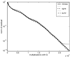
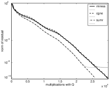
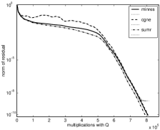
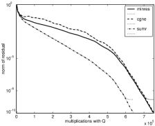
Figure 3: Propagator computation: Convergence of MINRES for (5), CGNE for (21) and SUMR for (4). Left column is for $\rho=1.01$, right column for $\rho=1.1$. The upper plots are for configuration A, the lower for configuration B.

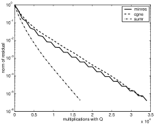
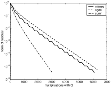
Figure 4: Propagator computation: Convergence of MINRES for (5), CGNE for (21) and SUMR for (4). Left plot is for a $8^{4}$ lattice, right plot for a $16^{4}$ lattice.

MINRES and CGNE behave very similarly on configuration A. This is to be expected, since the hermitian indefinite matrix $D_{h}$ is maximally indefinite, so that for an arbitrary right hand side the squaring of the matrix inherent in $D_{n}$ should not significantly increase the number of required iterations.

SUMR always performs best. The savings compared to MINRES and CGNE depend on $\rho$, $\beta$ and the lattice size and reached up to 50%.

As a side remark, let us mention that the dichotomy between hermitian indefinite and non-hermitian positive definite formulations is also a field of study in other areas. For example, FRS98 investigates the effect of multiplying some rows of a hermitian matrix with minus one in the context of solving augmented systems of the form

$$\left(\begin{array}[]{cc}A&B\\ B^{T}&0\\ \end{array}\right)\left(\begin{array}[]{c}x\\ y\\ \end{array}\right)=\left(\begin{array}[]{cc}b\\ 0\\ \end{array}\right)\Longleftrightarrow\left(\begin{array}[]{cc}A&B\\ -B^{T}&0\\ \end{array}\right)\left(\begin{array}[]{c}x\\ y\\ \end{array}\right)=\left(\begin{array}[]{cc}b\\ 0\\ \end{array}\right).$$

5.2 Dynamical simulations

Let us now turn to a dynamical simulation where we compute the solution $y^{*}$ from (15). The methods to be considered are CG for (15), a two-sweep SUMR-approach where we solve the two systems

$$D_{u}^{\dagger}x=b,\quad D_{u}y=x$$

using SUMR for both systems (note that $D_{u}^{\dagger}$ is of shifted unitary form, too), or a two-sweep MINRES-approach solving the two systems

$$D_{h}x=b,\quad D_{h}y=x.$$

It is now a bit more complicated to guarantee a comparable accuracy for each of the methods. Roughly speaking, we have to run both sweeps in the two-sweep methods to the given accuracy. Lemma 8 thus indicates that the two-sweep MINRES approach will not be competitive, whereas it does not determine which of two-sweep SUMR or CG is to be preferred. Our actual numerical experiments indicate that, in practice, CG is superior to two-sweep SUMR, see Figure 5.

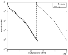
Figure 5: Dynamical simulation: Convergence of two-sweep SUMR (dash-dotted) and CG (solid) for (15) Left plot is for $\rho=1.01$, right plot for $\rho=1.1$. Both plots are for configuration A.

6 Conclusion

We have for the first time applied SUMR as the outer iteration when solving a propagator equation (4) for overlap fermions. Our theoretical analysis and the numerical results indicate that this new method is superior to CGNE as well as to MINRES on the symmetrized equation. In practice, savings tend to increase with larger values of $\rho$. We achieved savings of about 50% for physically interesting configurations.

We have also shown that when solving the squared equation (15) directly, as is required in a dynamical simulation, a two sweep approach using SUMR is not competitive to directly using CG with the squared operator. This is in contrast to the case of the Wilson fermion matrix, where it was shown in FHNLS94 that the two-sweep approach using BiCGstab performs better than CG.

In the context of the overall inner-outer iteration scheme, additional issues arise. In particular, one should answer the question of how accurately the result of the inner iteration (evaluating the product of $\hbox{\rm\,sign}(Q)$ with a vector) is really needed. This issue will be addressed in a forthcoming paper, ACE03 .

Acknowledgements. G.A. is supported under Li701/4-1 (RESH Forschergruppe FOR 240/4-1). N.C. enjoys support from the EU Research and Training Network HPRN-CT-2000-00145 “Hadron Properties from Lattice QCD”.

7 Definitions

The Wilson-Dirac matrix reads $M=I-\kappa D_{W}$ where

$$(D_{W})_{nm}=\sum_{\mu}(I-\gamma_{\mu})\otimes U_{\mu}(n)\delta_{n,m-\mu}+(I+\gamma_{\mu})\otimes U^{\dagger}_{\mu}(n-\mu)\delta_{n,m+\mu}$$ (25)

The Euclidean $\gamma$-matrices in the chiral representation are given as:

$${\gamma_{1}}:=\left[{\begin{array}[]{rrrr}0&0&i&0\\ 0&0&0&i\\ -i&0&0&0\\ 0&-i&0&0\end{array}}\right]{\gamma_{2}}:=\left[{\begin{array}[]{rrrr}0&0&-1&0\\ 0&0&0&1\\ -1&0&0&0\\ 0&1&0&0\end{array}}\right]{\gamma_{3}}:=\left[{\begin{array}[]{rrrr}0&0&0&i\\ 0&0&-i&0\\ 0&i&0&0\\ -i&0&0&0\end{array}}\right]{\gamma_{4}}:=\left[{\begin{array}[]{rrrr}0&0&0&1\\ 0&0&1&0\\ 0&1&0&0\\ 1&0&0&0\end{array}}\right].$$

The hermitian form of the Wilson-Dirac matrix is given by

$$Q=\gamma_{5}\,M,$$ (26)

with $\gamma_{5}$ defined as the product

$$\gamma_{5}:=\gamma_{1}\gamma_{2}\gamma_{3}\gamma_{4}=\left[{\begin{array}[]{rrrr}1&0&0&0\\ 0&1&0&0\\ 0&0&-1&0\\ 0&0&0&-1\end{array}}\right].$$ (27)

8 Massive Overlap Operator

Following Neuberger  hep-lat/9710089 , one can write the massive overlap operator as

$$D_{N}(\mu)=c\left((1+\mu)I+(1-\mu)M(M^{\dagger}M)^{-\frac{1}{2}}\right).$$ (28)

The normalisation $c$ can be absorbed into the fermion renormalisation, and will not contribute to any physics. For convenience, we have set $c=1/(1-\mu)$. Thus, the regularizing parameter $\rho$ as defined in eq. (2) is related to $\mu$ by

$$\rho=(1+\mu)/(1-\mu).$$ (29)

The physical mass of the fermion is then given by

$$m_{f}=\frac{2\mu}{\kappa(1-\mu)}.$$ (30)

References

- [1] G. Arnold, N. Cundy, J. van den Eshof, A. Frommer, S. Krieg, Th. Lippert, and K. Schäfer. Numerical methods for the QCD overlap operator: III. nested iterations. to appear.
- [2] R. G. Edwards, U. M. Heller, and R. Narayanan. A study of practical implementations of the overlap-dirac operator in four dimensions. Nucl. Phys., B540:457–471, 1999.
- [3] B. Fischer, A. Ramage, D. J. Silvester, and A. J. Wathen. Minimum residual methods for augmented systems. BIT, 38(3):527–543, 1998.
- [4] A. Frommer, V. Hannemann, B. Nöckel, Th. Lippert, and K. Schilling. Accelerating wilson fermion matrix inversions by means of the stabilized biconjugate gradient algorithm. Int. J. of Mod. Phys. C, 5(6):1073–1088, 1994.
- [5] U. Glässner, S. Güsken, Th. Lippert, G. Ritzenhöfer, K. Schilling, and A. Frommer. How to compute Green’s functions for entire mass trajectories within Krylov solvers. Int. J. Mod. Phys., C7:635, 1996.
- [6] G. H. Golub and C. F. Van Loan. Matrix Computations. The John Hopkins University Press, Baltimore, London, 3rd edition, 1996.
- [7] A. Greenbaum. Iterative Methods for Solving Linear Systems, volume 17 of Frontiers in Applied Mathematics. Society for Industrial and Applied Mathematics (SIAM), Philadelphia, PA, 1997.
- [8] C. F. Jagels and L. Reichel. A fast minimal residual algorithm for shifted unitary matrices. Numer. Linear Algebra Appl., 1(6):555–570, 1994.
- [9] R. Narayanan and H. Neuberger. An alternative to domain wall fermions. Phys. Rev., D62:074504, 2000.
- [10] H. Neuberger. Vector like gauge theories with almost massless fermions on the lattice. Phys. Rev., D57:5417–5433, 1998.
- [11] C. C. Paige and M. Wei. History and generality of the decomposition. Linear Algebra Appl., 208/209:303–326, 1994.
- [12] J. van den Eshof, A. Frommer, Th. Lippert, K. Schilling, and H.A. van der Vorst. Numerical methods for the QCD overlap operator: I. sign-function and error bounds. Comput. Phys. Comm., 146:203–224, 2002.