Lattice calculation of gluon screening masses

Abstract

We study $SU(3)$ gluon electric and magnetic masses at finite temperatures using quenched lattice QCD on a $20^{2}\times 32\times 6$ lattice. We focus on temperature regions between $T=T_{c}$ and $6T_{c}$, which are realized in BNL Relativistic Heavy Ion Collider and CERN Large Hadron Collider experiments. Stochastic quantization with a gauge-fixing term is employed to calculate gluon propagators. The temperature dependence of the electric mass is found to be consistent with the hard-thermal-loop perturbation, and the magnetic mass has finite values in the temperature region of interest. Both screening masses have little gauge parameter dependence. The behavior of the gluon propagators is very different in confinement/deconfinement physics. The short distance magnetic part behaves like a confined propagator even in the deconfinement phase. A simulation with a larger lattice, $32^{2}\times 48\times 6$, shows that the magnetic mass has a stronger finite size effect than the electric mass.

I Introduction

One of the most interesting features of QCD (quantum chromodynamics) is the transition from the confinement to the deconfinement phase. In this new state of QCD, quarks and gluons confined in the hadron at zero temperature move freely when the system reaches a sufficiently high temperature. The quark gluon plasma (QGP) was realized at high temperature in the early universe, and is expected to be produced in heavy-ion collision experiments at the CERN Super Proton Synchrotron (SPS), BNL Relativistic Heavy Ion Collider (RHIC), and CERN Large Hadron Collider (LHC). Thus it is an urgent task to accumulate theoretical knowledge about the QGP.

The massless gluon in the QGP medium is changed into a dressed massive gluon after quantum corrections. The screening effect is characterized by a mass pole of the propagator and is closely related to thermal QCD phenomenology. One example is a screened heavy quark potential, which is frequently discussed in relation to $J/\psi$ or $\Upsilon$ suppression. For calculations of jet quenching, which might be a fingerprint of a QGP, a model including the electric and magnetic masses has been proposed wang . A nonperturbative quantitative study in the vicinity of $T_{c}$ and up to several times $T_{c}$ is of great importance for understanding QGP physics.

The thermal field theory Gross ; Kapusta ; Bellac is the most basic method of studying the QGP and has provided many informative observations. At zero temperature, many calculations based on perturbative QCD have described experiment results Muta and there is no doubt that QCD is a theory of strong interaction. It is natural to employ the perturbative approach to thermal QCD. Because of the asymptotic freedom at high temperature, the coupling constant is expected to become small enough to carry out the perturbations. In such a high energy state, quarks and gluons must behave as an ideal gas; yet this simple consideration is spoiled by an infrared divergence Linde , which is known to bear a hierarchy on the energy scale in the QGP system Kapusta ; Bellac . One usually defines $1/T$ as a perturbative length scale, and furthermore $1/gT$ must be introduced as an electric (Debye) scale, whose influence appears as a Yukawa-type potential rather than a Coulomb-like one, and $1/g^{2}T$ as a magnetic scale. In QCD, the magnetic mass, which cannot be accessed perturbatively, acts as a cutoff factor in the infrared problem and consequently becomes an essential element of thermal QCD.

The QCD coupling constant strength near the critical temperature $T_{c}$ is still of the order of 1. Therefore perturbation theory is not applicable. However, these regions are currently being investigated with great interest in much theoretical and experimental research. After hard-thermal-loop (HTL) resummation was consistently formulated by Braaten and Pisarski, there were several improvements BP ; Niegawa for unsolved problems. Comparison of this method with lattice numerical data has been reported; one-loop HTL calculations of the free energy of a QGP are in good agreement with the lattice numerical result Andersen ; Andersen2 . However, a recent two-loop HTL calculation indicates that it does not yet have adequate convergence Andersen3 . As another approach, 3D reduction theory has also been widely studied and has yielded some promising arguments Kajantie , but this method, which is defined only for the high temperature limit, cannot be applied to confinement/deconfinement physics.

For reliable phenomenological analyses of high energy heavy-ion collisions, it is important to obtain information on the magnetic and electric masses of gluons nonperturbatively; a numerical study of lattice QCD as a first-principles calculation should play an important role here.

There have been many lattice studies of finite-temperature QCD, but only a few calculations of the electric and magnetic screening masses can be found in the literature Ogilvie , other than for the case of color $SU(2)$ Heller ; Cucchieri . The electric mass has been estimated from the Polyakov loop correlation functions to obtain the screened heavy-quark-antiquark potential Irback ; Gao ; Kaczmarek .

The main aim of our study is to obtain reliable $SU(3)$ electric and magnetic masses through large-scale lattice QCD simulations and to reveal their temperature dependence saito . We also compare our numerical data with the predictions of leading order perturbation (LOP), HTL resummation, and other analyses.

Since our mass extraction is based on measuring a gauge dependent gluon propagator, it is important to check the gauge invariance of both screening masses Cucchieri2 . This test is essential particularly for the magnetic mass because it has a poor definition in the frame of the perturbation.

Gluons are essential ingredients in QCD dynamics, and QCD undergoes a phase transition from the confinement to the deconfinement phase when the temperature increases. Therefore, we expect gluon propagators to show different behavior in each phase, and their study provides information on confinement/deconfinement dynamics Nakamura2 .

We measure gluon propagators, which depend on the gauge used, and therefore a gauge-fixing procedure is indispensable. However, gauge fixing on the lattice is difficult practically and conceptually. Usually, gauge fixing is carried out by the iterative technique Mandula , and it is very time consuming. The conceptual difficulty is that the gauge is not uniquely fixed; this is known as the Gribov copy problem Gribov . In order to overcome these difficulties, we adopt here a stochastic quantization with Zwanziger’s gauge-fixing term Zwanziger ; Seiler ; Mizutani , instead of the path integral method.

In this paper, we extend our previous results from the $20^{2}\times 32\times 6$ lattice simulations saito to the level that the present computer power can reach; we add more detailed values for the electric and magnetic masses and results at higher temperature from the larger lattice $32^{2}\times 48\times 6$ simulation. We also give a detailed description of the algorithm employed in this study. In Sec. II, we describe the stochastic gauge quantization together with the Gribov copy problem. The definitions of the gluon propagator and electric and magnetic masses are given. A large part of Sec. III is devoted to our simulation results on the small lattice $20^{2}\times 32\times 6$. First we describe all input parameters of the simulation and the statistics needed to measure reliable gluon propagators. Then we show the gluon behavior and the electric and magnetic masses extracted from it. The gauge dependence check and temperature dependence for both screening masses are also given. Finally, we compare the numerical data with the perturbative argument, add the higher temperature result, and comment on the finite volume effect. Section IV gives the conclusions.

The main part of the calculation was carried out on the SX-5(NEC) vector-parallel computer of RCNP(CMC), Osaka University. We used a parallel queue with 4, 8 and 16 CPUs and required about six months to complete this work.

II Stochastic gauge fixing on lattices and gluon propagators

II.1 Lattice gauge action

The lattice regularization scheme of QCD is the gauge invariant Euclidean theory which enables us to perform a nonperturbative calculation based on the Monte Carlo numerical technique Wilson . The simplest standard Wilson gauge action of lattice QCD can be defined from the continuum QCD as

$$S_{g}=\beta\sum(1-\frac{1}{3}\mbox{Re Tr}\left[U_{\nu}(x)U_{\mu}(x+\hat{\nu})U^{\dagger}_{\nu}(x+\hat{\mu})U^{\dagger}_{\mu}(x)\right]),\\ \hskip 5.69046pt\beta=\frac{2N_{c}}{g^{2}}.$$ (1)

Here a link variable, $U_{\mu}(x)$, stands for the $SU(3)$ color gauge field:

$$U_{\mu}(x)=e^{iga_{\mu}A_{\mu}(x)},$$ (2)

where $a_{\mu}$ is the lattice spacing, i.e, the lattice cutoff, and $A_{\mu}$ represents the gauge potential of the gluon. In this study, we adopt the quenched lattice simulation (pure gauge QCD) without a dynamical quark effect, using Eq. (1).

II.2 Gauge fixing and Gribov copy on lattices

We are interested in a direct calculation of the gluon propagator, and the extraction of electric and magnetic screening masses from it. Therefore we must fix the gauge of the gluon fields on the lattice, where the gauge transformation is given by

$$U_{\mu}(x)\rightarrow\omega^{\dagger}(x)U_{\mu}(x)\omega(x+\hat{\mu}).$$ (3)

$\omega$ stands for a gauge rotation matrix $\in SU(3)$ on the lattice.

In this study, we focus on a Lorentz-type gauge, which is defined in the continuum as

$$\partial_{\mu}A_{\mu}(x)=0,$$ (4)

while in the discrete lattice theory

$$\Delta^{a}(x)\equiv\sum_{\mu=1}^{4}2\mbox{ Im Tr }t^{a}\{U_{\mu}(x)-U_{\mu}(x-\hat{\mu})\}=0.$$ (5)

Here $t^{a}$ is the $SU(N)$ generator with the relation $\mbox{Tr}[t^{a}t^{b}]=\frac{1}{2}\delta^{ab}$. The above condition (5) is equivalent to

$$\begin{array}[]{lll}\delta_{\omega}I&=&0,\\ I&\equiv&\sum_{x,\mu}\mbox{Re Tr}\omega^{\dagger}(x)U_{\mu}(x)\omega(x+\hat{\mu}).\end{array}$$ (6)

Wilson Wilson80 and Mandula and Ogilvie Mandula suggested the following condition for the gauge fixing method on the lattice:

$$\mbox{Max.}_{\omega}I.$$ (7)

The continuum version of Eq. (7) was discussed in Refs. Maskawa and Semenov .

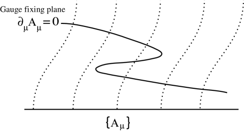
Figure 1: Gribov Gribov pointed out that a gauge is not uniquely fixed for non-Abelian theories, which is called the Gribov copy problem. This does not appear in the perturbative frame. The existence of the Gribov copy has been confirmed in several works Nakamura ; Hioki ; Bornyakov .

The conditions (6) and (7) are not equivalent to each other since there may be local maxima or minima of $I$ which satisfy Eq. (6). The gauge-fixing configuration cannot be uniquely fixed; this is called the “Gribov copy” Gribov and is illustrated in Fig. 1. If we study this problem using a numerical lattice simulation based on the iterative procedure, it is very difficult to find a true maximum.

II.3 Stochastic gauge fixing

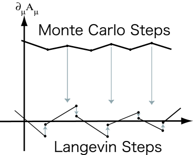
Figure 2: The figure illustrates the gauge-fixing procedure by the Wilson-Mandula-Ogilvie iterative method and by stochastic gauge fixing. Gray arrows indicate the gauge rotation for each algorithm. In the first algorithm, Monte Carlo update steps are performed without restriction on the $\partial_{\mu}A_{\mu}=0$ plane. When a gauge fixed configuration is needed, the gauge configuration is rotated to the gauge-fixed plane, $\partial_{\mu}A_{\mu}=0$, by iteration Mandula . On the other hand, in the case of Langevin gauge fixing, configurations are updated by fluctuation around $\partial_{\mu}A_{\mu}=0$.

Our approach to the gauge-fixing procedure is to use the stochastic gauge quantization instead of the Monte Carlo path integral. The stochastic quantization is based on the Langevin equation which introduces virtual time in addition to the Euclidean coordinate. Zwanziger introduced a gauge-fixing term as

$$\frac{dA_{\mu}^{a}}{d\tau}=-\frac{\delta S}{\delta A_{\mu}^{a}}+\frac{1}{\alpha}D^{ab}_{\mu}(A)\partial_{\nu}A_{\nu}^{b}+\eta_{\mu}^{a},$$ (8)

where $D_{\mu}^{ab}(A)$ is a covariant derivative, $\tau$ stands for Langevin time, and $\eta$ is a Gaussian noise term. The second term on the right-hand side is a gauge-fixing term. $\alpha$ is a gauge parameter; $\alpha=0$ corresponds to the Lorentz gauge and $\alpha=1$ to the Feynman gauge.

Mizutani and Nakamura Mizutani developed the lattice version of the stochastic gauge fixing. The link variables are rotated through the following gauge transformation depending on the virtual time:

$$U_{\mu}(x,\tau+\Delta\tau)=\omega^{\dagger}(x,\tau)e^{if_{\mu}^{a}t^{a}}U_{\mu}(x,\tau)\omega(x+\hat{\mu},\tau).$$ (9)

Here $f$ stands for the force

$$f_{\mu}^{a}=-\frac{\partial S}{\partial A_{\mu}^{a}}\Delta\tau+\eta^{a}\sqrt{\Delta\tau},$$ (10)

and the gauge rotation matrix is given by

$$\omega=e^{i\beta\Delta^{a}t^{a}\Delta\tau/\alpha}.$$ (11)

If $\omega=I$, Eq. (9) is a lattice Langevin process. Gauge rotation, Eq. (9), with Eq. (11), leads to the gauge fixing term as $\Delta\tau\rightarrow 0$. Equation (9) means that the gauge rotation and Langevin step are executed alternately, as illustrated in Fig. 2.

In this stochastic quantization with Lorentz-type gauge fixing, $\Delta^{a}$ fluctuates around the gauge-fixing plane $\Delta^{a}=0$. For example, when we take $\alpha=1.0$ and $\Delta\tau=0.01$, $\Delta^{a}$ on $4^{3}\times 8$ with $\beta=6.0$ behaves as shown in Fig. 3. We confirm that $\Delta^{a}$ fluctuates around $\Delta^{a}=0$ which indicates that good gauge fixing is achieved.

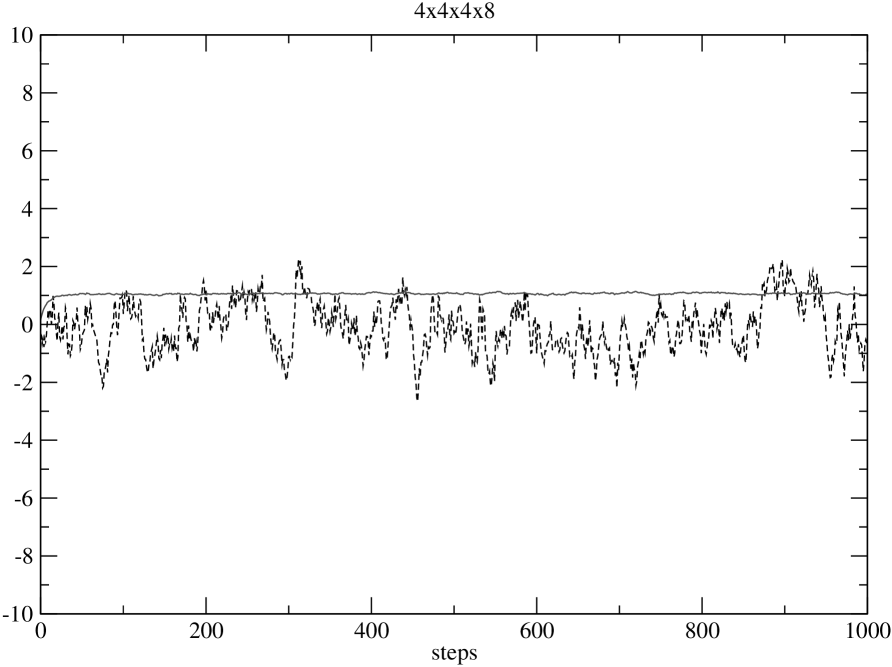
Figure 3: These data are produced on the lattice $4^{3}\times 8$ with $\Delta\tau=0.01$(Langevin step interval), $\alpha=1.0$ (gauge parameter) at $\beta=6.0$. The solid line means the average of $\sum_{x,a}\{\Delta^{a}(x)\}^{2}$, while the dashed line is the value of $\Delta^{1}(1)$. $\Delta^{a}$ fluctuates around $\Delta^{a}=0$ and gauge configurations are sufficiently fixed on the $\partial_{\mu}A_{\mu}=0$ plane.

There are two reasons for using the stochastic gauge-fixing method in this study. One is a practical issue. When we use the standard Wilson-Mandula gauge-fixing method Mandula , the iterative procedure is applied to accepted gauge configurations for each Monte Carlo step in Fig. 2. Then the number of iterations is unpredictable, particularly for large lattices. On the other hand, in algorithm (9), we simultaneously repeat the step of update and gauge rotation in Fig. 2 and are free from the convergence problem of gauge fixing. Therefore we can estimate the CPU time precisely. Moreover, this algorithm, in which the gauge parameter $\alpha$ can be changed at will, is advantageous when testing gauge invariance.

A conceptual problem is the Gribov ambiguity Gribov . The algorithm has a noteworthy feature, i.e., the second term of Eq. (8) gives rise to a configuration such that

$$\begin{array}[]{lll}\frac{d}{d\tau}\sum_{x}\Delta^{2}&<&0\mbox{\ in\ \ \ \ \ \ }\Omega\\ &>&0\mbox{\ out of\ }\Omega.\end{array}$$ (12)

Here $\Omega$ stands for the Gribov region,

$$\mbox{Gribov\ region}:\Omega\equiv\{A_{\mu}^{a}(x)|\partial_{\mu}A_{\mu}^{a}(x)=0,-\partial_{\mu}D_{\mu}^{ab}>0\}.$$ (13)

That is, the stochastic gauge-fixing term is attractive (repulsive) inside (outside) the Gribov region Zwanziger ; Seiler if we start from the trivial configuration $\{A_{\mu}=0\}$. Although our algorithm may not completely eliminate copies, we conclude that it is a more effective method.

Since the update algorithm described here is not as popular as the Metropolis or pseudo-heat-bath method, we show the autocorrelation of the Polyakov lines $L(\tau)L(\tau+n\tau)$ in Fig. 4 together with that of the pseudo-heat-bath.

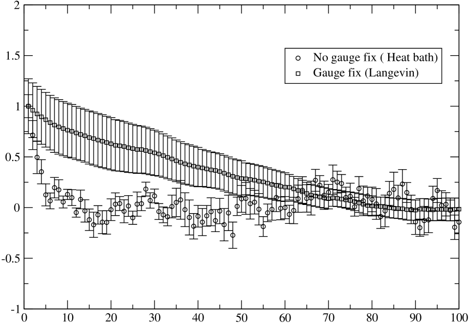
Figure 4: Autocorrelation of the Polyakov loops for the Langevin algorithm with the stochastic gauge fixing ($\Delta\tau=0.03$) and the pseudo-heat-bath update algorithms as a function of the iteration steps. This calculation is done at $\beta=6.1$ on the $8^{3}\times 4$ lattice.

II.4 Definition of gluon propagators

We define the gauge field $A_{\mu}(x)$ in terms of the link variables as

$$A_{\mu}(x)=2\sum_{a}t^{a}\mbox{Im}\mbox{Tr}t^{a}U_{\mu}(x).$$ (14)

We calculate massless gluon correlation functions with finite momentum,

$$G_{\mu\nu}(p_{x},p_{y},p_{t},z)=\langle\mbox{Tr}A_{\mu}(p_{x},p_{y},p_{t},z)A_{\nu}(-p_{x},-p_{y},-p_{t},0)\rangle.$$ (15)

In our study, to avoid a mixture of the longitudinal and transverse modes, we adopt the transverse conditions $p_{i}\cdot A_{i}=0$ and measure the partially Fourier transformed propagator including one momentum $p_{x}=2\pi/N_{x}$ or $p_{y}=2\pi/N_{y}$ Nakamura . We will obtain the gluon mass using a lattice energy momentum relation. This is different from other calculations Heller ; Ogilvie , where the mass extraction from zero momentum propagator was studied.

In thermal perturbative QCD Gross ; Kapusta ; Bellac , the electric mass is defined from the temporal part of the gluon polarization tensor $\Pi_{\mu\nu}$, while its spatial part is considered as the magnetic mass. Thus we can construct an electric propagator using a temporal one:

$$G_{e}(p,z)\sim\frac{1}{2}\left[G_{tt}(\frac{2\pi}{N_{x}},0,0,z)+G_{tt}(0,\frac{2\pi}{N_{y}},0,z)\right].$$ (16)

In the same way, a magnetic propagator is defined by spatial components:

$$G_{m}(p,z)\sim\frac{1}{2}\left[G_{xx}(0,\frac{2\pi}{N_{y}},0,z)+G_{yy}(\frac{2\pi}{N_{x}},0,0,z)\right].$$ (17)

Because the screening mass is given as a pole of the denominator of the momentum space propagator, $1/(p^{2}+m^{2})$, $G_{e}(z)$ and $G_{m}(z)$ are expected to behave as exponential damping functions in the z direction on distances, $Z\geqslant 1/T$ with the masses,

$$G_{e(m)}(z)\sim e^{-E_{e(m)}(p)z}.$$ (18)

III Results

III.1 Simulation parameters

We use mainly the lattice of the size $N_{x}N_{y}N_{z}N_{t}=20^{2}\times 32\times 6$ which satisfies the condition $N_{x}\geqslant 3N_{t}$. On this lattice the long range area corresponds to $z\geqslant 1/T$ and thus reliable information for screening physics may be produced.

We summarize lattice cutoff values and the corresponding temperature in Table 1. Varying $\beta$, i.e., the lattice coupling constant, we change the temperature $T=1/N_{t}a$. The pure gauge lattice with $N_{t}=6$ has critical $\beta_{c}\sim 5.89$ and we adopt $T_{c}\sim 256$ Boyd as the critical temperature. To estimate the lattice cutoff value, we employ the results in Refs. QCD_TARO ; Allton .

In addition, we prepare a lattice of the size $32^{2}\times 48\times 6$ in order to investigate the finite size effect of screening masses, and to obtain them at higher temperature.

Table 1: We estimate a lattice cutoff and its temperature scale by using mainly QCD_TARO fit function QCD_TARO ; Allton . We adopt $T_{c}\sim 256$ Boyd .

$\beta$	$a^{-1}$[GeV]	T[MeV]	$T/T_{c}$	$\beta$	$a^{-1}$[GeV]	T[MeV]	$T/T_{c}$
5.8	1.33	222	0.86	6.4	3.52	586	2.29
5.90	1.62	270	1.05	6.5	4.12	690	2.69
5.95	1.77	295	1.15	6.6	4.60	767	2.99
6.0	2.04	340	1.32	6.7	5.24	874	3.41
6.05	2.09	349	1.36	6.8	5.96	994	3.88
6.1	2.27	378	1.47	6.9	6.76	1128	4.40
6.2	2.64	447	1.74	7.0	7.64	1274	4.97
6.3	3.05	509	1.99	7.1	8.61	1436	5.61

III.2 Necessary statistics to obtain reliable gluon propagators

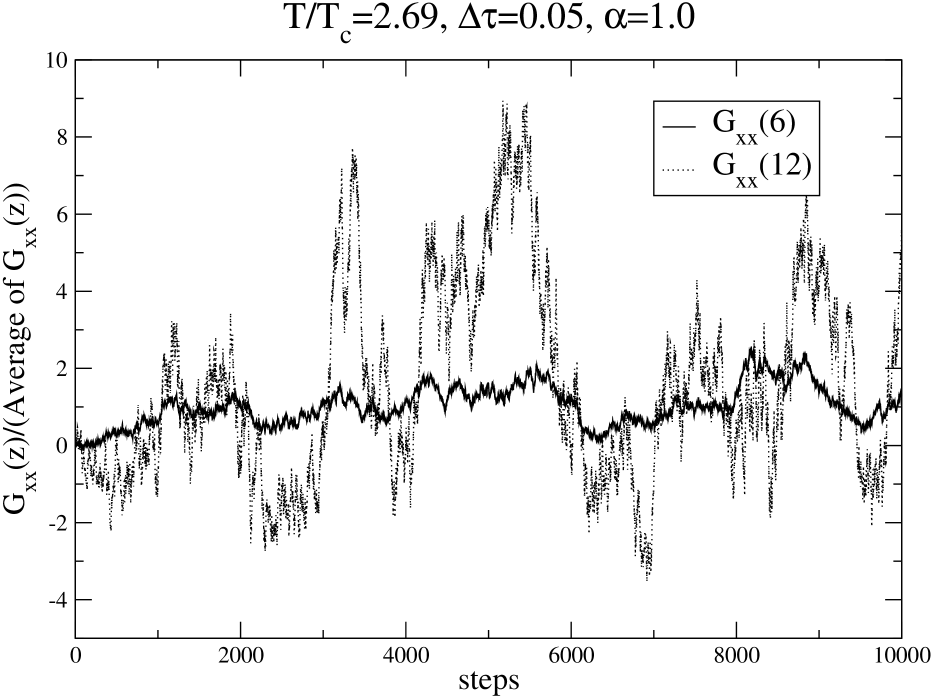
Figure 5: Typical gluon propagator behavior as a function of Langevin steps on the lattice $20^{2}\times 32\times 6$. We find that fluctuations of $G_{xx}(12)$ are much larger than those of $G_{xx}(6)$. In order to investigate the screening effect, the long range contribution should be adopted. Consequently, we need a large number of statistics.

We observe a large fluctuation of the gauge propagators, particularly at long distances, i.e., we suffer from a long autocorrelation time. We show in Fig. 5 the typical behavior of gluon propagators $G(z)$ as a function of the Langevin step. In order to analyze the gluon propagator and measure the screening masses we require $0.2-0.4\times 10^{6}$ steps as the typical number of simulation data.

III.3 Gluon propagators

Although the gluon propagator itself is gauge dependent, it gives us some insights into the gluon dynamics of the confinement/deconfinement physics.

The electric propagator is shown in Fig. 6 , where the free massless propagator is also shown by the dashed line. Gluons at short distances, i.e., $z<6=1/T$, have very similar behavior to the free propagator. However, at long distances, gluon propagators decrease more rapidly than the free one. This indicates that the electric screening mass does not vanish at all temperatures.

Comparing data below and above $T_{c}$, we find that the dynamics of the gluon is completely different in the confinement and deconfinement regions. The electric gluon mass in the confinement region becomes heavier; the electric gluon is completely screened in the confinement regions. This was first observed in Ref. Nakamura2 . Consequently, we cannot employ the assumption Eq. (18). On the contrary, the propagator in the deconfinement regions decreases exponentially even at long distances with a finite mass.

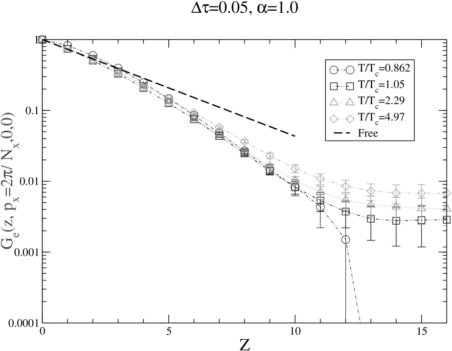
Figure 6: The electric propagator in the confinement (circle) and deconfinement regions (other symbols) with $P_{x(y)}=2\pi/N_{x(y)}$. All propagators are found to become massive compared with the free propagator (long dashed line). In the confinement regions, the propagator at long distances behaves like a very massive particle and vanishes, whereas the propagator beyond $T_{c}$ has a finite mass.

Similar behavior is seen in the magnetic parts in Fig. 7; although the long distance magnetic gluons have large errors here, all magnetic gluons are found to be massive at long distances in the confinement/deconfinement phase, and their effective mass in the confinement phase is heavier. We notice that the short distance behavior of magnetic gluons in the deconfinement regions looks unconventional. The magnetic gluon propagators follow a convex curve at short distances while the electric ones do not. The magnetic gluons behave as if they had an imaginary screening mass or negative spectral function, which may be the reason why the magnetic mass is not screened at least in LOP calculation.

As clearly seen in Fig. 7 and as we discuss below, the effective mass of the magnetic mass is $z$ dependent. We take the value around $z=1/T$ as the electric case, since it is a relevant quantity at finite temperature screening.

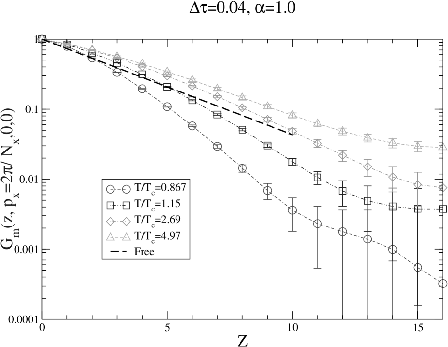
Figure 7: The magnetic gluon propagator in the confinement (circle) and deconfinement regions (other symbols) with $P_{x(y)}=2\pi/N_{x(y)}$. Although the magnetic gluon propagators in this figure have large errors at long distances, they seem to have similar behavior to the electric part, except for the short distance behavior in the deconfinement regions.

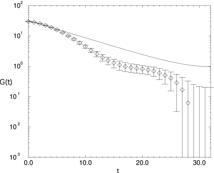
Figure 8: Transverse gluon propagator, $G_{T}(t)$ with ${\bf p}=((2\pi/N_{x}),0,0)$, on $48^{3}\times 64$ at $\beta=6.8$ (confinement phase). Solid line represents the free propagator Nakamura2 .

Gluons are essential ingredient of QCD but they are confined below $T_{c}$. As shown in Fig. 8, their propagator is convex upward at several regions. This is possible only when the spectral function is not positive definite. This peculiar behavior was first observed in Ref. Mandula and confirmed in Ref. Nakamura95 . The feature does not contradict the fundamental postulate of quantum field theories, because gluons in the confinement region are not physically observable particles. Instead, this is a glimpse of the confinement mechanism in the infrared region which is still far from our understanding. Gribov’s conjecture for the gluon propagator

$$G(p)\sim\frac{Z}{p^{2}+b^{4}/p^{2}},$$ (19)

vanishes at $p^{2}=0$, and its Fourier transformation to the coordinate space is not convex downward,

$$\tilde{G}(t)\sim\frac{Z}{r}e^{rt\cos\phi}\cos(rt\sin\phi+\phi),$$ (20)

where $r\equiv(|\vec{p}|^{4}+b^{4})^{1/4}$ and $\phi\equiv\frac{1}{2}\tan^{-1}({b^{2}}/{\vec{p}^{2}})$. The upward convex shape of the gluon propagators in the deconfinement region may provide us with hints about the glue dynamics.

Below the critical temperature $T_{c}$, we obtain a similar result even for electric gluons at short distances. This seems natural since the perturbative argument in the confinement regions is generally not suitable and the confining correlation function would also give the negative spectral function.

III.4 Mass as a pole

To obtain the screening mass from the propagators, the following formula is used:

$$G_{e(m)}\sim\cosh[E_{e(m)}(p)(z-N_{z}/2)].$$ (21)

We employ data for $z\geqslant 1/T(=N_{t}a)$, because the screening effect occurs at sufficiently long distances. All fittings are done from $z=6$ to $N_{z}/2$, and $\chi^{2}/NDF\sim O(1)$, where $NDF$ indicates the number of degrees of freedom.

To obtain the final result at $\Delta\tau=0$, we must extrapolate the data with respect to Langevin step width. The Runge-Kutta algorithm is applied to reduce the finite Langevin step $\Delta\tau$ dependence Batrouni . We perform simulations for a set of parameters with $\Delta\tau=0.03\sim 0.05$. Table 2 and Fig. 9 represent $E(p)$ measured here versus $\Delta\tau$. The slight dependence of $\Delta\tau$ enables us to use a linear function when fitting data.

Figure 9: $\Delta\tau$ dependence of masses is slight. Finally to obtain a final value at $\Delta\tau=0$, we use the linear function for the extrapolation.

We finally obtain the mass from $E(p)$ by the following lattice energy-momentum relation Heller :

$$\sinh^{2}\frac{Ea}{2}=\sinh^{2}\frac{ma}{2}+\sum_{i=1}^{3}\sin^{2}\frac{p_{i}a}{2}.$$ (22)

Table 2: This shows the typical example of the Langevin step dependence at $T/T_{c}=2.69$. For all simulations for $\Delta\tau=0.03-0.05$, approximately $0.2-0.4\times 10^{6}$ steps (measurements) are used after eliminating about $3000-5000$ steps as thermalization. “${\bf p}\neq 0$” means including the momentum $P_{x(y)}=2\pi/N_{x(y)}$. We extrapolate these data to $\Delta\tau=0$ and then obtain $m_{e}a(p_{\mu}=0)=0.470(38)$ and $m_{m}a(p_{\mu}=0)=0.199(52)$ using lattice energy-momentum relation.

$\Delta\tau$	Number of steps	$m_{m}a({\bf p}\neq 0)$	$m_{e}a({\bf p}\neq 0)$
0.05	275000	0.400(08)	0.544(22)
0.045	240000	0.364(12)	0.527(21)
0.04	380000	0.381(11)	0.508(21)
0.035	280000	0.369(08)	0.551(24)
0.0325	300000	0.336(09)	0.565(28)
0.03	320000	0.367(14)	0.551(24)
0.00		0.369(46)	0.561(40)

III.5 Gauge invariance

The screening mass is physical and expected to be gauge invariant. However, since the gluon propagators defined by Eqs. (16) and (17) are gauge dependent, it is important to check whether the screening masses obtained here are gauge invariant or not. In addition, since the magnetic mass cannot be defined by a perturbative calculation, it is particularly important to check its gauge dependence. In Fig. 10, we show the gauge parameter $\alpha$ dependence of electric and magnetic masses. The gauge dependence of both screening masses is found to be very slight, namely, the result strongly suggests that they are gauge invariant and physical observables.

Figure 10: Gauge dependence for electric and magnetic screening masses. Gauge dependence of both screening masses is very slight.

III.6 Temperature dependence

We study the temperature dependence of the screening mass in the range $T/T_{c}=1-6$ which would be realized in high energy heavy-ion collision experiments such as RHIC or LHC Muller . Table 3 and Fig. 11 show electric and magnetic masses as a function of the temperature. The magnetic part definitely has nonzero mass in this temperature region. As $T$ increases, both $m_{e(m)}/T$ decrease monotonically, and at almost all temperatures, the magnetic mass is less than the electric one, except very near $T_{c}$ where the electric mass decreases very quickly as $T$ approaches $T_{c}$.

Table 3: Temperature dependence of the electric and magnetic masses which are extrapolated to the Langevin step $\Delta\tau=0$.

$T/T_{c}$	$m_{e}/T$	$m_{m}/T$	$T/T_{c}$	$m_{e}/T$	$m_{m}/T$
1.05	1.506(438)	2.802(054)	2.69	2.820(228)	1.194(312)
1.15	2.694(288)	2.484(258)	2.99	2.892(234)	1.590(318)
1.32	3.348(408)	2.406(246)	3.41	2.190(450)	0.960(168)
1.36	2.904(336)	1.986(296)	3.88	2.292(222)	0.852(318)
1.47	3.138(342)	1.866(222)	4.40	2.598(168)	1.134(414)
1.74	2.700(426)	1.620(300)	4.97	2.310(084)	0.804(638)
1.99	2.898(498)	1.608(270)	5.61	2.106(390)	0.486(336)
2.29	2.484(234)	0.990(264)

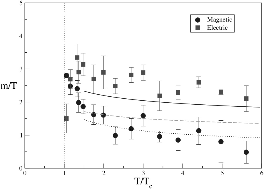
Figure 11: Temperature dependence of electric and magnetic screening masses. The dotted line is fitted by the assumption, $m_{g}\sim g^{2}T$. For the electric mass, the dashed and solid lines represent LOP and HTL resummation results, respectively.

III.7 Comparison with LOP and HTL resummation results

We perform a fitting analysis for our numerical results using the following ansatz:

$$\frac{m_{e}}{T}=C_{e}g(T),\hskip 7.11317pt\frac{m_{m}}{T}=C_{m}g^{2}(T),$$ (23)

whose g dependence is predicted by the perturbative and 3D reduction analysis Kapusta ; Bellac and we assume $C_{e}$ and $C_{m}$ are free parameters. In the following discussion, the data above $T\sim 1.5T_{c}$ are used. Here we use the running couplings as

$$g^{2}(\mu)=\frac{1}{2b_{0}\log(\mu/\Lambda)}\left(1-\frac{b_{1}}{2b_{0}}\frac{\log(2\log\mu/\Lambda)}{\log(\mu/\Lambda)}\right),$$ (24)

and we set $\mu=2\pi T$, which is the Matsubara frequency as the renormalization point and $\Lambda=1.03T_{c}$ Andersen as the QCD mass scale. $b_{0}$ and $b_{1}$ are the first two universal coefficients of the renormalization group,

$$b_{0}=11N_{c}/48\pi^{2},\quad b_{1}=(34/3)(N_{c}/(16\pi^{2}))^{2}.$$ (25)

As a result, we obtain

$$\begin{array}[]{clc}C_{e}&=1.63(3),&\chi^{2}/\mbox{NDF}=0.715,\\ C_{m}&=0.482(31),&\chi^{2}/\mbox{NDF}=0.979.\end{array}$$ (26)

The scalings expected in Eq. (23) for electric and magnetic masses are found to work well. However, the magnitude of $C_{e}$ is larger than $C_{e}^{LOP}=1$. On the other hand, for magnetic mass, a self-consistent inclusion technique in Ref. Alexanian gives $m_{g}=0.568g^{2}T$, which is close to our fitting result.

The HTL resummation technique applying the free energy of hot gluon plasma has been widely discussed Andersen ; Andersen2 . Rebhan gave a formula for the electric mass in the one-loop HTL perturbation theory Rebhan and for the case of $SU(3)$,

$$m_{e}^{2}=m_{e,0}^{2}\left[1+\frac{3g}{2\pi}\frac{m_{e}}{m_{e,0}}\left(\log\frac{2m_{e}}{m_{m}}-\frac{1}{2}\right)+O(g^{2})\right],m_{e,0}=gT.$$ (27)

Here we assume the magnetic mass to be of the order of $g^{2}$. Substituting our fitted value for $m_{m}$, we can solve the above equation iteratively. In Fig. 11, we show this HTL resummation together with the LOP result. The HTL result gives a better description than the naive perturbation, upon comparing with our numerical experiment.

The electric mass was obtained also by a heavy $q\bar{q}$ potential from the $SU(3)$ Polyakov loop correlator at finite temperature in Refs. Gao ; Kaczmarek . Our results here are inconsistent with theirs, since the mass extraction from the heavy $q\bar{q}$ potential cannot be consistently performed due to ambiguity of its fitting assumption. In addition, a 3D reduction argument Kajantie has shown that $m_{e}/gT$ goes down when $T$ increases, but even at $T\sim 1000\Lambda_{\overline{MS}}$ the electric mass is still about $3m_{e,0}$. This observation agrees qualitatively with our analysis.

III.8 Higher T and finite size effect

Although the main result in this paper is based on studies for the small lattice size $20^{2}\times 32\times 6$ as discussed in the previous section, we additionally perform the simulation on the large lattice $32^{2}\times 48\times 6$ to go to higher temperature regions and to check the finite-size effect of the screening masses. However, as the lattice size increases, the behavior of the long distance gluon cannot be controlled because of a large fluctuation. A typical result on the large lattice is shown in Fig. 12. Even after the $0.3-0.4\times 10^{6}$ measurements, we could not determine the electric gluon propagator at long distances ($z\geqslant 16$), while the magnetic gluon is properly correlated. Nevertheless, provided that we adopt only the data for the intermediate regions above $z=6$ until the disappearance of the propagator, we obtain similar results for the electric and magnetic masses as seen in Fig. 12 in the same temperature regions.

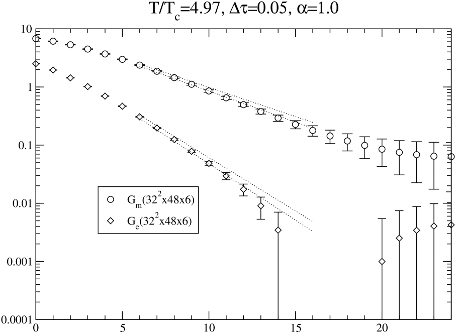
Figure 12: Typical electric and magnetic propagators on the large lattice $32^{2}\times 48\times 6$ (open), and the data for $20^{2}\times 32\times 6$ (band between dotted lines with error) are reproduced by using the values in Table 3. Both calculations give very similar value for electric and magnetic parts.

Using the criterion describing above, we may consistently obtain both screening masses on the large lattice, and can argue that the magnetic mass has a stronger finite-size effect than the electric one. $E(p)$ appearing in Eq.(17) are shown in Table 4 at $T/T_{c}=8.99$ and $16.12$. The momenta for the small and large lattices are $p_{x}=2\pi/N_{x}\sim 0.314$ and $p_{x}=2\pi/N_{x}\sim 0.196$, respectively; namely, the result on the small lattice implies that the magnetic mass at high temperature ($T/T_{c}>5$) seems to be going to zero, while on the large lattice it remains finite.

Although it is very difficult to measure the long distance gluon propagators, we can add the higher temperature results ( $T/T_{c}=8.99,16.12$ ) summarized in Table 5. In Fig. 13 we again fit the data including these new points. The fit for the large lattice data by Eq. (23) hence results in

$$\begin{array}[]{clc}C_{e}&=1.69(4),&\chi^{2}/NDF=0.66,\\ C_{m}&=0.549(16),&\chi^{2}/NDF=1.27\end{array}$$ (28)

These results are shown in Fig. 13. It should be noticed that $C_{e}$ is the same value as given in Eq. (26), while $C_{m}$ $\sim 10\%$ larger on the large lattice and is very close to $m_{g}=0.568g^{2}T$ calculated by the self-consistent inclusion technique in Ref. Alexanian .

Table 4: Data extracted from the small and large lattices in the same coupling regions, $\beta=7.5$ and $\beta=8.0$.

$\beta$	$\Delta\tau$	$m_{m}a({\bf p}\neq 0)$	$m_{e}a({\bf p}\neq 0)$
small lattice size $20^{2}\times 32\times 6$
7.5	0.05	0.301(15)	0.455(09)
8.0	0.04	0.311(09)	0.457(14)
large lattice size $32^{2}\times 48\times 6$
7.5	0.05	0.231(03)	0.433(08)
8.0	0.04	0.214(04)	0.406(14)

Table 5: Simulation parameters and screening masses for the large lattice $32^{2}\times 48\times 6$. Lattice scales are estimated by Refs. QCD_TARO ; Allton .

$\beta$	$a^{-1}$[GeV]	T[MeV]	$T/T_{c}$	$m_{m}/T$	$m_{e}/T$
7.0	7.64	1274	4.97	1.128(78)	2.556(156)
7.5	13.8	2303	8.99	1.014(54)	2.178(144)
8.0	24.7	4127	16.12	0.984(60)	2.256(120)

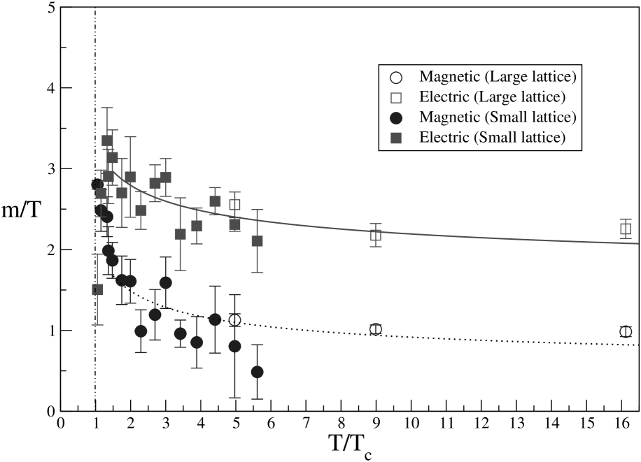
Figure 13: The temperature dependence including higher temperature points on the large lattice $32^{2}\times 48\times 6$.

IV Conclusions

We have measured the gluon propagators and obtained the electric and magnetic masses by lattice QCD simulations in the quenched approximation for SU(3) between $T=T_{c}$ and $6T_{c}$. Features of the QGP in this temperature region will be extensively studied theoretically and experimentally in the near future.

Our screening mass studies are the first reliable measurement in $SU(3)$ lattice calculation. We mainly investigate the temperature dependence for the electric and magnetic masses which do not vanish on $20^{2}\times 32\times 6$ lattices. In all temperature regions we find that the electric mass $m_{e}$ is always larger than the magnetic one $m_{m}$, except near critical temperature point. As the temperature goes down toward $T_{c}$, $m_{e}/T$ drops down quickly, while $m_{m}/T$ is still going up. Consequently, using data above $T/T_{c}\sim 1.5$ we conclude that the scalings $m_{e}\sim gT$ and $m_{m}\sim g^{2}T$ work well. Furthermore, a HTL resummation calculation has recently been developed and compared with nonperturbative lattice simulations. We have also compared our numerical results with LOP and HTL resummation and find a good improvement of the HTL electric mass. These comparison studies of $SU(3)$ screening masses qualitatively seem to agree with the case of $SU(2)$ Heller .

The electric masses obtained here are not consistent with those obtained by heavy $q\bar{q}$ potential calculations from an $SU(3)$ Polyakov loop correlator at finite temperature in Refs. Gao ; Kaczmarek . In Ref. Kaczmarek , the authors did extensive analyses with three different temporal extents and two different gauge actions, obtaining a very reliable potential as a function of the temperature. They observe that the potential above $T_{c}$ cannot be described properly by the leading order perturbation calculation up to a few $T_{c}$: They exclude the two-gluon exchange as the dominant screening mechanism, and suggest that some kind of one-gluon exchange may describe the potential effectively as a result of the complex interaction, and that at about $(1.5-3)T_{c}$ a mixture of one- and two-gluon exchange may explain the behavior. Therefore, due to the ambiguity of the fitting assumptions, it is not clear whether we can compare our screening masses directly with those obtained by the potential calculation.

In order to investigate the nature of the QGP, especially the excitation modes in the plasma, Datta and Gupta recently calculated glueball masses at finite temperature and made an interesting observation. They measured the screening masses of $A_{1}^{++}$ (scalar) and $A_{2}^{--}$ (glueball), which allow two- and three-gluon exchange, and their ratio $\sim 1.7$ is near 3/2. The $A_{2}^{--}$ mass is twice that obtained by Kaczmarek et al, and shows similar temperature dependence. There are now several nonperturbative methods to study QGP: our direct measurement of the gluon propagators, glueball screening masses, and Polyakov line correlators. These analyses strongly suggest that the QGP above $T_{c}$ is far from a free gas and has a nontrivial structure. Much more detailed analyses in future are highly desirable.

The screening mass on the lattice is extracted from the gauge dependent propagator, and the magnetic mass is not well defined in perturbation theory. We have nonperturbatively confirmed the gauge invariance of both screening masses. In Ref. Cucchieri2 it was reported that the $SU(2)$ magnetic propagator exhibits a complicated gauge dependent structure at low momentum. Therefore, since the gauge dependence for the screening masses is investigated within Lorentz-type gauge fixing based on stochastic gauge quantization in this study, we plan to extend our analysis to a simulation with Coulomb-type gauge fixing.

We have seen a qualitative difference of the gluon dynamics between the confinement and deconfinement phase by direct propagator measurement. The electric and magnetic gluons in the confinement phase indicate a very massive particle behavior, while after the phase transition, they have a finite mass. In addition, in the deconfinement phase, the magnetic gluon at short distances seems to be still in the confinement phase. This may be related to the difficulty of the perturbative argument for spatial gluon components and the fact that a magnetic Wilson loop gives non-zero spatial string tension even at high temperatures Fingberg .

The magnetic mass has been the subject of many discussions. Perturbatively, it is difficult to handle. To our knowledge, there is no complete perturbative calculation which is free from any assumption or model. The naive expectation is that it vanishes, but it is necessary to have a finite value as a cutoff factor in the infrared regime. On the other hand, the finite spatial string tension even at $T>T_{c}$ indicates “confinement” in the magnetic sector.

Our screening gluon magnetic propagators indeed show nontrivial behavior. At very short distances, this may be consistent with massless behavior, but at finite distance we cannot fit them by a simple ansatz. The behavior is distance dependent. Confinement is a long range property, and the propagators there drop. Therefore it will be a very interesting task in future to investigate the magnetic propagators at very long distance.

We calculated the gluon propagators on the larger lattice $32^{2}\times 48\times 6$ and observed a large error and strange behavior at long distances. Nevertheless, the screening masses were estimated, and we find that the magnetic mass is sensitive to the lattice size effect. Thus on a too small lattice we cannot deal with the magnetic mass consistently. Moreover, the simulations even at higher temperature $T/T_{c}\sim 9$ and $16$ show that nonperturbative results are far from LOP. This observation is compatible with that of Ref. Kajantie ; Heller .

For quantization with gauge fixing, stochastic gauge fixing was adopted. We think the stochastic gauge fixing has better features to reduce some of the difficulties of nonperturbative gauge fixing. It is consequently possible to do a practical simulation of gluon screenings effectively. However, we also see that the gluon propagators have large fluctuations and unexpected behavior at long distances and may need further calculations.

The color screening data we obtained here are useful information for QGP phenomenology, for instance, jet quenching or the heavy quark potential. We plan to study the $q\bar{q}$ as well as the $qq$ potential relating a baryon bound state, a nonperturbative QCD vertex calculation, quark propagators, etc., using stochastic gauge fixing, which will help us to understand QGP.

V Acknowledgement

We would like to thank A. Ni$\acute{\mbox{e}}$gawa, S. Muroya, T. Inagaki and I. Pushkina for many helpful discussions. The calculation was done on an SX-5(NEC) vector-parallel computer. We really appreciate the warm hospitality and support of the RCNP administrators. An HPC computer at INSAM, Hiroshima University was also used. This work was supported by Grant-in-Aids for Scientific Research by Monbu-Kagaku-sho (No.11440080, No. 12554008, and No. 13135216)

References

- (1) X.N. Wang, Phys. Lett. B 485, 157 (2000).
- (2) D.J. Gross, R.D. Pisarski and L.G. Yaffe, Rev. Mod. Phys. 53, 43 (1981).
- (3) J.I. Kapusta, Finite-Temperature Field Theory (Cambridge monographs on mathematical physics, Cambridge University Press, Cambridge, 1989).
- (4) M. Le Bellac, Thermal Field Theory (Cambridge monographs on mathematical physics, Cambridge University Press, Cambridge, 1996).
- (5) T. Muta, FUNDATION OF QUANTUM CHROMODYNAMICS 2ND EDITION (World Scientific Lecture Notes in Physics - Vol. 57 World Scientific Publishing Co. Pte. Ltd., 1998).
- (6) A.D. Lind, Phys. Lett. 96B, 289 (1980).
- (7) R.D. Pisarski, Phys. Rev. Lett. 63, 1129 (1989); E. Braaten and R.D. Pisarski, Phys. Rev. Lett. 64, 1338 (1990); E. Braaten and R.D. Pisarski, Nucl. Phys. B337, 569 (1990).
- (8) A. Nigawa, Phys. Rev. Lett. 73, 2023 (1994).
- (9) J.O. Andersen, E. Braaten and M. Strickland, Phys. Rev. Lett. 83, 2139 (1999).
- (10) J.-P. Blaizot, E. Iancu and A. Rebhan, Phys. Rev. Lett. 83, 2906 (1999); Phys. Lett. B 470, 181 (1999); Phys. Rev. D 63, 065003 (2001).
- (11) J.O. Andersen, E. Braaten, E. Petitgirard and M. Strickland, Phys. Rev. D 66, 085016 (2002).
- (12) K. Kajantie, M. Laine, J. Peisa, A. Rajantie, K. Rummukainen and M. Shaposhnikov, Nucl. Phys. B(Proc.Suppl.) 63A-C, 418 (1998); Phys. Rev. Lett. 79, 3130 (1997).
- (13) J.E. Mandula and M. Ogilvie, Phys. Lett. B 201, 117 (1988).
- (14) U.M. Heller, F. Karsch and J. Rank, Phys. Lett. B 355, 511 (1995); Phys. Rev. D 57, 1438 (1998).
- (15) A. Cucchieri, F. Karsch and P. Petreczky, Phys. Lett. B 497 80 (2001).
- (16) A. Irbck, P. Lacock, D. Miller, B. Petersson and T. Reisz, Nucl. Phys. B 363, 34 (1991).
- (17) M. Gao, Phys. Rev. D 41, 626 (1990).
- (18) O. Kaczmarek, F. Karsch, E. Laermann and M. Ltgemeier, Phys. Rev. D 62, 034021 (2000).
- (19) A. Nakamura, I. Pushkina, T. Saito and S. Sakai, Phys. Lett. B, 549, 133(2002).
- (20) A. Cucchieri, F. Karsch and P. Petreczky, Phys. Rev. D 64 036001 (2001).
- (21) A. Nakamura, Prog. Theor. Phys. Suppl. 131, 585, 1998.
- (22) J.E. Mandula and M. Ogilvie B 185, 127 (1987).
- (23) V.N. Gribov, Nucl. Phys. B139, 1 (1978); Gribov Theory of Quark Confinement, Ed. by J. Nyiri, (World Scientific, Singapore, 2001).
- (24) D. Zwanziger, Nucl. Phys. B192, 259 (1981).
- (25) E. Seiler, I.O. Stamatescu and D. Zwanziger, Nucl. Phys. B239, 177 (1984).
- (26) A. Nakamura and M. Mizutani, Vistas in Astronomy (Pergamon Press), vol. 37, 305 (1993); M. Mizutani and A. Nakamura, Nucl. Phys. B(Proc. Suppl.) 34, 253 (1994).
- (27) K.G. Wilson Phys. Rev. D 10 , 2445 (1974).
- (28) K.G. Wilson, in Recent Developments in Gauge Theories, ed. G. t’Hooft (Plenum Press, New York, 1980), 363.
- (29) T. Maskawa and H. Nakajima, Prog. Theor. Phys. 63 641 (1980).
- (30) Semenov-Tyan-Shanskii and Franke, Zapiski Nauchnykh Seminarov, Leningradskage Otdelleniya Mathemat. Instituta im Steklov ANSSSR Vol. 120, 159 (1982).
- (31) A. Nakamura and M. Plewnia, Phys. Lett. B 255, 274 (1991).
- (32) S. Hioki, S. Kitahara, Y. Matsubara, O. Miyamura, S. Ohno and T. Suzuki, Phys. Lett. B 271, 201 (1991).
- (33) V.G. Bornyakov, V.K. Mitrjushkin, M. Muller-Preussker and F. Pahl, Phys. Lett. B 317, 596 (1993).
- (34) QCDTARO collaboration, K. Akemi, et al., Phys. Rev. Lett. 71, 3063 (1993).
- (35) C.R. Allton, hep-lat/9610016 (1996).
- (36) G. Boyd, J. Engels, F. Karsch, E. Laermann, C. Legeland, M. Ltgemeier and B. Petersson, Phys. Rev. Lett. 75, 4169 (1995).
- (37) H.Aiso, M.Fukuda, T.Iwamiya, M.Mizutani, A.Nakamura, T.Nakamura and M.Yoshida, Nucl.Phys. B (Proc.Suppl.) 42, 1995, 899; H.Aiso, M.Fukuda, T.Iwamiya, A.Nakamura, T.Nakamura and M.Yoshida Prog. Theor. Physics, Suppl. No.122, 1996, 123.
- (38) A. Ukawa and M. Fukugita, Phys. Rev. Lett. 55, 1854 (1985); G.G. Batrouni, G.R. Katz, A.S. Kronfeld, G.P. Lepage, B. Svetitsky and K.G. Wilson, Phys. Rev. D 32, 2736 (1985).
- (39) B. Mller, Nucl. Phys. A 630 , 461c, (1998).
- (40) G. Alexanian and V.P. Nair, Phys. Lett. B 352, 435 (1995).
- (41) A.K. Rebhan, Phys. Rev. D 48, R3967 (1993); Nucl. Phys. B430, 319 (1994).
- (42) S. Datta and S. Gupta, Phys. Rev. D 67, 054503 (2003).
- (43) G. S. Bali, J. Fingberg, U. M. Heller, F. Karsch, and K. Schilling, Phys. Rev. Lett. 71, 3059(1993).