Abstract

We determine the relative pion mass shift $M_{\pi}(L)/M_{\pi}-1$ due to the finite spatial extent $L$ of the box by means of two-flavor chiral perturbation theory and the one-particle Lüscher formula. We use as input the expression for the infinite volume $\pi\pi$ forward scattering amplitude up to next-to-next-to-leading order and can therefore control the convergence of the chiral series. A comparison to the full leading order chiral expression for the pion mass in finite volume allows us to check the size of subleading terms in the large-$L$ expansion.

1 Introduction

Shifts in particle masses and matrix elements due to the finite extent of the box are systematic effects in the Monte Carlo treatment of any lattice field theory. These shifts become particularly large when the spectrum contains light particles, and apply to all particles, no matter how heavy, provided they couple to the light ones. In QCD with light quarks, e.g. the nucleon mass receives such a correction, which disappears only as the product of the pion mass times the length of the box ($M_{\pi}L$) gets large.

Fortunately, as long as pions are light, chiral symmetry imposes strong constraints on the way observables deviate from their infinite-volume limit: chiral perturbation theory (CHPT) allows one to perform a systematic expansion around this limit and hence to control the finite-volume effects analytically [1, 2, 4, 3, 5]. In some cases one can directly translate the results of finite volume simulations into information about infinite-volume quantities without any need to extrapolate in the box size $L$ [6]. CHPT is an expansion in the pion mass and particle momenta which have to be small in comparison to the chiral symmetry breaking scale, usually identified with $4\pi F_{\pi}$. The conditions of applicability read

$${p\over 4\pi F_{\pi}}\ll 1\;,\quad{M_{\pi}\over 4\pi F_{\pi}}\ll 1\;.$$ (1)

Particles inside a box of spatial length $L$ with periodic boundary conditions and comparatively large or infinite time extent may only have discrete values of their spatial momenta, $p_{k}=2\pi n_{k}/L$ with $n_{k}\in\mathbf{Z}$. In this case the first condition in (1) becomes a bound on the box size:

$$L\gg{1\over 2F_{\pi}}\sim 1\,\mathrm{fm}\;.$$ (2)

Note that these conditions have no say whether $L$ is large compared to the Compton wavelength of the pion or not. Both options are acceptable [5], but they imply different ways to organize the chiral series:

$$M_{\pi}L\gg 1\quad\leftrightarrow\quad\mbox{``$p$-expansion''}\,\,$$ (3)

$$M_{\pi}L\ll 1\quad\leftrightarrow\quad\mbox{``$\epsilon$-expansion''}\;.$$ (4)

We shall here restrict ourselves to the former case but investigate what the conditions (1b, 2) mean quantitatively, by considering more than the leading order in the chiral expansion. The underlying assumption is that CHPT itself will tell us when the conditions of applicability are not respected any more, via a bad convergence behavior.

Figure 1: The mass shift due to quantized momenta in the self-energy corrections amounts to a finite-size effect from pion exchange “around the world” (left), depicted by a “thermal insertion” (cross) in diagrammatic language (right).

In this paper we study the pion mass, $M_{\pi}(L)$, defined as eigenvalue of the QCD Hamiltonian in a $L\!\times\!L\!\times\!L$ box (with periodic boundary conditions), as it is extracted on an Euclidean lattice for sufficiently large time $T$. The finite volume shift, $M_{\pi}(L)-M_{\pi}$, is – in coordinate space view – due to the possibility of the pion wrapping “around the world” or – in momentum space view – due to the discrete momenta, as depicted in Fig. 1. The ultraviolet properties of the theory are untouched – with toroidal boundary conditions no new counterterms are introduced and the finite size effect is automatically finite. Our goal is to study the shift $M_{\pi}(L)-M_{\pi}$ (with $M_{\pi}$ we always denote the infinite-volume value) as a function of $M_{\pi}$ and $L$. A preliminary account has been given in [7]. Here, we include one more order in the chiral expansion (at large $L$) and carefully analyze the uncertainty due to the errors of the QCD low-energy constants involved. In addition, we compare to the full one-loop result by Gasser and Leutwyler (which is leading in the chiral expansion, but includes the large-$L$ suppressed terms).

2 The pion mass in finite volume

2.1 Finite volume calculations in CHPT

In a series of remarkable papers [2, 4, 3], Gasser and Leutwyler have shown that chiral symmetry does severely constrain physical observables at low energy even if the system is confined to a finite box. The only condition is that the box length $L$ must be several fermi, cf. (2).

Using the method of the effective chiral Lagrangian, one can establish low energy theorems for physical quantities of interest, which have the generic form

$$Q = Q_{0}\left[1+\xi q_{1}+\xi^{2}q_{2}+O(\xi^{3})\right]$$ (5)

$$\xi \equiv {M_{\pi}^{2}\over(4\pi F_{\pi})^{2}}\;\;,$$ (6)

and the coefficients $q_{i}$ are quantities of order one in the chiral expansion. They depend on the low–energy constants (LEC), on ratios of momenta and quark masses, and, in finite volume, on

$$\lambda\equiv M_{\pi}L\;\;.$$ (7)

$n$	1	2	3	4	5	6	7	8	9	10	11	12	13	14	15	16	17	18	19	20
$m(n)$	6	12	8	6	24	24	0	12	30	24	24	8	24	48	0	6	48	36	24	24

Table 1: The multiplicities $m(n)$ in (11) for $n\leq 20$.

For the pion mass and decay constant, the coefficient $q_{1}$ in the $p$-expansion (3) has been explicitly evaluated in Ref. [2],

$$M_{\pi}(L) = M_{\pi}\left[1+{1\over 2N_{\!f\,}}\xi\,\tilde{g}_{1}(\lambda)+O(\xi^{2})\right]$$ (8)

$$F_{\pi}(L) = \;F_{\pi}\left[1-\;{N_{\!f\,}\over 2}\,\xi\,\tilde{g}_{1}(\lambda)+O(\xi^{2})\right]$$ (9)

with

$$\tilde{g}_{1}(\lambda)=\sum\nolimits^{\prime}\int_{0}^{\infty}dx\;e^{-{1\over x}-{x\over 4}(n_{1}^{2}+n_{2}^{2}+n_{3}^{2})\lambda^{2}}\;\;,$$ (10)

where the sum runs over all integer values of $n_{1,2,3}$, excluding the term with $(n_{1},n_{2},n_{3})=(0,0,0)$ as indicated by the prime over the summation symbol. For a given value of $n:=n_{1}^{2}+n_{2}^{2}+n_{3}^{2}$ the integral can be performed analytically, and we can rewrite $\tilde{g}_{1}$ as

$$\tilde{g}_{1}(\lambda)=\sum_{n=1}^{\infty}{4m(n)\over\sqrt{n}\,\lambda}\;K_{1}\left(\sqrt{n}\,\lambda\right)\;\;,$$ (11)

where $K_{1}$ is a Bessel function of the second kind and the multiplicity $m(n)$ indicates how many times the value $n$ is generated in the sum in Eq. (10). The values of $m(n)$ for $n\leq 20$ are given in Table 1. For large argument the Bessel function $K_{1}$ drops exponentially: $K_{1}(x)\simeq e^{-x}/\sqrt{x}$. Since $\lambda\!\gg\!1$ by assumption, the sum (11) converges very rapidly, and it is easy to check how many terms are needed to get a good approximation for the complete sum. The convergence of the chiral expansion, on the other hand, is more difficult to test: the coefficient $q_{2}$ has not yet been calculated neither for $M_{\pi}$ nor for $F_{\pi}$. This would require a full two–loop calculation in CHPT in finite volume. We are going to argue, however, that there is a fast and reliable way to check the convergence of the chiral expansion – a way that is based on a formula due to Lüscher [8] which we will discuss in detail. Before doing so, it is useful to rearrange Eq. (8, 9) by making explicit the expansion of each coefficient $q_{m}$ in a series of rapidly decreasing exponentials (in $\lambda$)

$$M_{\pi}(L) = M_{\pi}\Big{[}1+\left(\xi q^{M}_{11}+\xi^{2}q^{M}_{21}+O(\xi^{3})\right)K_{1}(\lambda)$$ (12)

$$\qquad\;\;\,+\left(\xi q^{M}_{12}+\xi^{2}q^{M}_{22}+O(\xi^{3})\right)K_{1}(\sqrt{2}\lambda)+\;\ldots\Big{]}$$

$$= M_{\pi}\left[1+\sum_{m=1}^{\infty}\sum_{n=1}^{\infty}\xi^{m}q^{M}_{mn}\,K_{1}(\sqrt{n}\,\lambda)\right]$$

$$F_{\pi}(L) = \,F_{\pi}\,\left[1+\sum_{m=1}^{\infty}\sum_{n=1}^{\infty}\xi^{m}q^{F}_{mn}\,K_{1}(\sqrt{n}\,\lambda)\right]\;\;,$$ (13)

where at leading order in the chiral expansion the coefficients $q_{1n}$ follow from Table 1,

$$q^{M}_{1n}=+{2m(n)\over N_{\!f\,}\sqrt{n}\,\lambda}\;\;,\qquad\qquad q^{F}_{1n}=-{2N_{\!f\,}m(n)\over\sqrt{n}\,\lambda}\;\;.$$ (14)

Notice that the Bessel functions that we have factored out in Eqs. (12, 13) need not necessarily appear in this form also at higher orders in the chiral expansion – the coefficients $q^{M,F}_{mn}$ are presumably complicated functions of $\lambda$, in general. We do expect, however, that also at higher orders the result may be expressed as a series of exponentials, whose leading asymptotic behavior should be captured by the Bessel functions in (12,13).

2.2 Lüscher’s formula for $M_{\pi}(L)$

Lüscher considered the problem of evaluating the finite size effects on a particle mass from a different point of view. Via graph–theoretic arguments he proved an elegant relation between the (Euclidean) finite volume mass shift and the (Minkowski space) $\pi\pi$ forward scattering amplitude $F(\nu)$ in infinite volume [8]:

$$M_{\pi}(L)-M_{\pi}=-{3\over 16\pi^{2}M_{\pi}L}\;\int_{-\infty}^{\infty}\!dy\;F({\rm i}y)\,e^{-\sqrt{M_{\pi}^{2}+y^{2}}\,L}+O(e^{-\overline{M}L})\;\;.$$ (15)

The integration runs along the imaginary axis, where the amplitude is far away from its cuts (cf. Fig. 2): only the real part of $F({\rm i}y)$ contributes to the integral. The one-particle Lüscher formula (15) is an asymptotic relation for large $L$; it is proven to all orders in perturbation theory for an arbitrary massive QFT, and the subleading piece is tamed by the bound $\overline{M}\!\geq\!\sqrt{3/2}\>M_{\pi}$ [8]. An extra term originating from the 3-particle vertex in the original formula [8] does not appear in our case, due to the odd intrinsic parity of the pion and parity conservation in QCD. Since eq. (15) builds on the unitarity of the theory, it holds only in full QCD. A variant for the quenched approximation is not known, if at all possible.

Figure 2: Integration contour in the complex $\nu$ plane where $\nu$ is the crossing variable in the (Minkowski space) forward scattering amplitude. The cut is generated only at NLO in the chiral expansion.

Neither the formula, nor its derivation make use of the chiral expansion (indeed the formula was derived before CHPT was applied to finite volume effects). However, for practical applications we need to insert an explicit, analytic representation for the $\pi\pi$ forward scattering amplitude, and for this we shall rely on CHPT. A comparison to the expression (12) shows that by inserting the chiral expansion for $F$ in (15) and evaluating the integral one can obtain the coefficients $q^{M}_{m1}$. If we write (extracting a factor $16\pi^{2}$ for later convenience)

$$F({\rm i}y)=16\pi^{2}\left[\xi F_{2}+\xi^{2}F_{4}+\xi^{3}F_{6}+O(\xi^{4})\right]\;\;,$$ (16)

the integration of the term $F_{2m}$ yields the coefficient $q^{M}_{m1}$. Since for 2 degenerate dynamical flavors the $\pi\pi$ scattering amplitude is known to next-to-next-to-leading order [9] in the chiral expansion, i.e. up to $F_{6}$, we can evaluate the coefficients $q^{M}_{m1}$, $m\!=\!1,2,3$ for $N_{\!f\,}\!=\!2$. All this without having to do a single new loop calculation in CHPT in finite volume.

We stress that the Lüscher formula is designed to yield the leading term in the large $L$ expansion: whenever the relative suppression factor

$${\mbox{subleading}\over\mbox{leading}}=O\Big{(}e^{-(\overline{M}-M_{\pi})L)}\Big{)}$$ (17)

is not small, subleading effects may be of practical relevance. In order to estimate subleading effects in the large $L$ expansion we will go back to the expansion of $\tilde{g}_{1}(\lambda)$.

The rest of this article is devoted to such a combined use of Lüscher’s formula (15) and the chiral expansion (16) for two-flavor QCD. It is useful to keep in mind that the chiral formulae contain low-energy constants that have been pinned down in real Minkowski space experiments; some stem indeed from $\pi\pi$ scattering data, which determine the amplitude in the physical region, e.g. for forward kinematics, on the cuts in Fig. 2. The very fact that the chiral expression for $F(\nu)$ holds in the whole complex $\nu$ plane is a key ingredient of this work – we rely on the good analyticity properties of the chiral amplitudes.

2.3 Combining CHPT and the Lüscher formula

The forward scattering amplitude which is needed in Lüscher’s formula can be expressed in terms of the isospin invariant amplitude $A(s,t,u)$ as follows

$$F(\nu) = T(2M_{\pi}(M_{\pi}+\nu),0,2M_{\pi}(M_{\pi}-\nu))$$

$$T(s,t,u) = A(s,t,u)+3A(t,s,u)+A(u,s,t)\;\;,$$ (18)

where the only independent kinematical variable $\nu$ reads

$$\;\;\nu\equiv{p_{a}\cdot p_{b}\over M_{\pi}}={s\over 2M_{\pi}}-M_{\pi}\;\;,$$ (19)

in terms of the momenta $p_{a,b}$ of the two initial pions. Since $A(s,t,u)$ is symmetric under $t,u$ exchange, the forward scattering amplitude is an even function of $\nu$: $F(\nu)\!=\!F(-\nu)$.

We find it convenient to use a dimensionless integration variable and introduce

$$\tilde{y}=y/M_{\pi}\;\;,\qquad\tilde{\nu}=\nu/M_{\pi}\;\;.$$ (20)

In these variables and with $N\!=\!16\pi^{2}$ the chiral expansion of the forward scattering amplitude is

$$F(\nu)=N\left[\xi F_{2}(\tilde{\nu})+\xi^{2}F_{4}(\tilde{\nu})+\xi^{3}F_{6}(\tilde{\nu})+O(\xi^{4})\right]\;\;.$$ (21)

If we combine Lüscher’s formula with the chiral expansion for $F$ we obtain a simple expression:

$${M_{\pi}(L)-M_{\pi}\over M_{\pi}} \equiv R_{M}(M_{\pi},L)\;\;,$$

$$R_{M}(M_{\pi},L) = -{3\over\lambda}\int_{-\infty}^{\infty}d\tilde{y}\;e^{-\sqrt{1+\tilde{y}^{2}}\,\lambda}\left[\xi F_{2}({\rm i}\tilde{y})+\xi^{2}F_{4}({\rm i}\tilde{y})+\xi^{3}F_{6}({\rm i}\tilde{y})+O(\xi^{4})\right]+\ldots$$ (22)

$$= -{3\over\lambda}\left[\xi I_{2}(\lambda)+\xi^{2}I_{4}(\lambda)+\xi^{3}I_{6}(\lambda)+O(\xi^{4})\right]+\ldots\;\;,$$

where the ellipsis indicate terms of order $e^{-\bar{M}_{\pi}L}$ and

$$I_{2m}(\lambda)=\int_{-\infty}^{\infty}d\tilde{y}\;e^{-\sqrt{1+\tilde{y}^{2}}\,\lambda}\,F_{2m}({\rm i}\tilde{y})\;\;.$$ (23)

Using the expression for $A$ in [9] (which is specific to $N_{\!f\,}=2$) and splitting its $b_{i}$ coefficients

$$\begin{array}[]{lcll}b_{i}&\equiv&\bar{b}_{i}/N&\mathrm{for}\quad i=1,\ldots,4\\ b_{i}&\equiv&\bar{b}_{i}/N^{2}&\mathrm{for}\quad i=5,6\\ \bar{b}_{i}&\equiv&\bar{b}_{i}^{0}+\xi\bar{b}_{i}^{1}&\mathrm{for}\quad i=1,\ldots,4\;\;,\end{array}$$ (24)

the calculation of the coefficients $I_{2m}$ in (22) can be made in large parts analytically:

$$I_{2}(\lambda) = -B^{0}(\lambda)$$

$$I_{4}(\lambda) = B^{0}(\lambda)\Big{(}5\bar{b}_{1}^{0}+4\bar{b}_{2}^{0}+8\bar{b}_{3}^{0}+8\bar{b}_{4}^{0}\Big{)}$$

$$+ B^{2}(\lambda)\Big{(}-8\bar{b}_{3}^{0}-56\bar{b}_{4}^{0}\Big{)}$$

$$+ {13\over 3}R_{0}^{0}(\lambda)-{16\over 3}R_{0}^{1}(\lambda)-{40\over 3}R_{0}^{2}(\lambda)$$

$$I_{6}(\lambda) = B^{0}(\lambda)\Big{(}5\bar{b}_{1}^{1}+4\bar{b}_{2}^{1}+8\bar{b}_{3}^{1}+8\bar{b}_{4}^{1}+16\bar{b}_{5}+16\bar{b}_{6}\Big{)}$$ (25)

$$+ B^{2}(\lambda)\Big{(}-8\bar{b}_{3}^{1}-56\bar{b}_{4}^{1}-48\bar{b}_{5}+16\bar{b}_{6}\Big{)}$$

$$+ R_{0}^{0}(\lambda)\Big{(}50+10\bar{b}_{1}^{0}+{56\over 3}\bar{b}_{2}^{0}+{104\over 3}\bar{b}_{3}^{0}+{56\over 3}\bar{b}_{4}^{0}\Big{)}$$

$$+ R_{0}^{1}(\lambda)\Big{(}-{1402\over 27}-{32\over 3}\bar{b}_{2}^{0}-{128\over 3}\bar{b}_{3}^{0}-{32\over 3}\bar{b}_{4}^{0}\Big{)}$$

$$+ R_{0}^{2}(\lambda)\Big{(}-{1756\over 27}-{80\over 3}\bar{b}_{2}^{0}-{392\over 3}\bar{b}_{3}^{0}+{136\over 3}\bar{b}_{4}^{0}\Big{)}$$

$$+ R_{0}^{3}(\lambda)\Big{(}-{116\over 27}+16\bar{b}_{3}^{0}-48\bar{b}_{4}^{0}\Big{)}$$

$$+ R_{1}^{0}(\lambda)\Big{(}{1\over 9}-{\pi^{2}\over 18}\Big{)}+R_{1}^{1}(\lambda)\Big{(}{128\over 9}-{\pi^{2}\over 72}\Big{)}+R_{1}^{2}(\lambda)\Big{(}-{100\over 9}-{\pi^{2}\over 24}\Big{)}$$

$$+ R_{2}^{0}(\lambda)\Big{(}{7\over 6}-{\pi^{2}\over 18}\Big{)}+R_{2}^{1}(\lambda)\Big{(}{16\over 9}+{7\pi^{2}\over 72}\Big{)}+R_{2}^{2}(\lambda)\Big{(}{\pi^{2}\over 24}\Big{)}$$

$$- {46\over 9}R_{3}^{0}(\lambda)-{32\over 9}R_{3}^{1}(\lambda)-{32\over 3}R_{3}^{2}(\lambda)$$

$$+ {40\over 3}R_{4}^{0}(\lambda)+{40\over 3}R_{4}^{1}(\lambda)\;\;,$$

where the integrals $B^{2k}$ admit a simple analytical representation

$$B^{2k}(\lambda) = \int_{-\infty}^{\infty}d\tilde{y}\;\tilde{y}^{2k}\,e^{-\sqrt{1+\tilde{y}^{2}}\lambda}={\Gamma(k+1/2)\over\Gamma(3/2)}\left({2\over\lambda}\right)^{k}K_{k+1}(\lambda)\;\;,$$

$$B^{0}(\lambda) = \,2\,K_{1}(\lambda)\;\;,$$

$$B^{2}(\lambda) = {2\over\lambda}K_{2}(\lambda)\;\;.$$ (26)

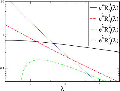
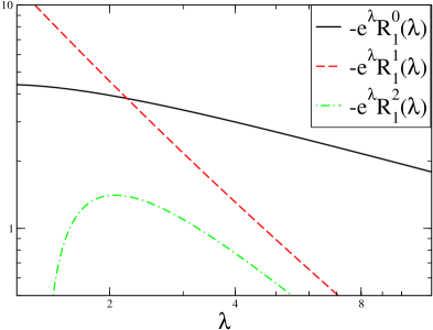
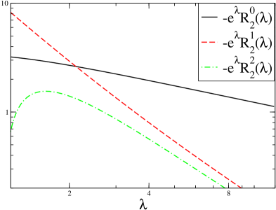
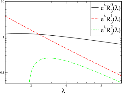
The integrals denoted by $R_{i}^{k}$, $i=0,\ldots,4$ are defined as follows

$$R_{i}^{k}(\lambda)=N^{2}\,\left\{{\mathrm{Re}\atop\mathrm{Im}}\right.\int_{-\infty}^{\infty}d\tilde{y}\;\tilde{y}^{k}\,e^{-\sqrt{1+\tilde{y}^{2}}\,\lambda}\,K_{i}^{\pi\pi}\left(2(1+{\rm i}\tilde{y})\right)\qquad\mathrm{for}\left\{{k\;\mathrm{even}\atop k\;\mathrm{odd}}\right.\\$$

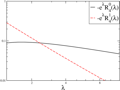
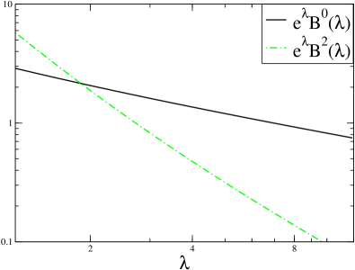
(the $K_{i}^{\pi\pi}$ functions appear in the $\pi\pi$ scattering amplitude at the two–loop level [9] – there they are defined without the $\pi\pi$ superscript – and collected in Appendix B) and can be easily calculated numerically, while an analytic representation is not available. The integrals $B^{2k}$ and $R_{i}^{k}$ are plotted in Fig. 3. As can be seen there, they are all of a similar magnitude – in the representation (22) the small parameter $\xi$ appears explicitly such that all the remaining coefficients are not expected to show any special hierarchy.

Figure 3: The integrals $B^{2k}$ and $R_{i}^{k}$ which are needed for the evaluation of the finite volume corrections to NNLO. The $B^{2k}$ are known analytically, the $R_{i}^{k}$ have been determined numerically.

The last ingredient needed for an evaluation of $R_{M}(M_{\pi},L)$ is the numerical values of the LEC which appear in the coefficients $\bar{b}_{i}$ (which are specific for $N_{\!f\,}=2$), and in $F_{\pi}$, if the latter needs to be computed from $M_{\pi}$. The expression of the $\bar{b}_{i}$ in terms of the relevant LEC can be found in the appendix. At order $p^{2}$ no LEC appears. At order $p^{4}$ four LEC appear: three of them were determined rather precisely in [10], whereas for the one that dictates the NLO quark mass dependence of $M_{\pi}^{2}$, we rely on the estimate in [1]. Altogether, this means that we use

$$\tilde{\ell}_{i} \equiv \log{\Lambda_{i}^{2}\over\mu^{2}}$$

$$\Lambda_{1} = 0.12\stackrel{{\scriptstyle+0.04}}{{{}_{-0.03}}}\;\,\mathrm{GeV}\;\;,\qquad\qquad\Lambda_{2}=1.20\stackrel{{\scriptstyle+0.06}}{{{}_{-0.06}}}\;\,\mathrm{GeV}\;\;,$$

$$\Lambda_{3} = 0.59\stackrel{{\scriptstyle+1.40}}{{{}_{-0.41}}}\;\,\mathrm{GeV}\;\;,\qquad\qquad\Lambda_{4}=1.25\stackrel{{\scriptstyle+0.15}}{{{}_{-0.13}}}\;\,\mathrm{GeV}\;\;.$$ (27)

At order $p^{6}$ six new LEC appear. Two of them were determined in [10], whereas for the remaining four we rely on the resonance saturation hypothesis [9], with a (conservative) 100% error estimate:

$$\tilde{r}_{1} = -1.5\times(1\pm 1)\;\;,\qquad\qquad\tilde{r}_{2}=3.2\times(1\pm 1)\;\;,$$

$$\tilde{r}_{3} = -4.2\times(1\pm 1)\;\;,\qquad\qquad\tilde{r}_{4}=-2.5\times(1\pm 1)\;\;,$$

$$\tilde{r}_{5} = 3.8\pm 1.0\;\;,\qquad\qquad\qquad\;\;\tilde{r}_{6}=1.0\pm 0.1\;\;.$$ (28)

Inserting these values and evaluating the corresponding $\bar{b}_{i}$ one can then determine the integrals $I_{2},...,I_{6}$ in the $\xi$-expansion (22), and hence $R_{M}(M_{\pi},L)$, the details being given in section 3 and the appendix.

3 Numerical evaluation

3.1 Quark mass dependence of $F_{\pi}$

In CHPT the expansion parameter is $\xi$, and in (12, 22) the finite volume effects have been expressed as a power series in this parameter. If, in a lattice calculation, both $M_{\pi}(L)$ and $F_{\pi}(L)$ have been determined, then the square of $M_{\pi}(L)/(4\pi F_{\pi}(L))$ may be taken as a first approximation to $\xi$, with iterative refinement through (12, 13). In order to give a numerical prediction with only $M_{\pi}$ as input, we must know how $\xi$ depends on the quark mass, or – equivalently – we are left with the problem of evaluating the pion mass dependence of $F_{\pi}$. The analytic expression of the latter is known to next–to–next–to leading order [11], and reads in our variables

$$F_{\pi} = F\Bigg{\{}1+X\Big{[}\tilde{L}+\tilde{\ell}_{4}\Big{]}+X^{2}\Big{[}-{3\over 4}\tilde{L}^{2}+\tilde{L}\Big{(}-{7\over 6}\tilde{\ell}_{1}-{4\over 3}\tilde{\ell}_{2}+\tilde{\ell}_{4}-{29\over 12}\Big{)}$$ (29)

$$\qquad\qquad\qquad\qquad\qquad\quad\;+{1\over 2}\tilde{\ell}_{3}\tilde{\ell}_{4}-{1\over 12}\tilde{\ell}_{1}-{1\over 3}\tilde{\ell}_{2}-{13\over 192}+\tilde{r}_{F}(\mu)\Big{]}\Bigg{\}}$$

where $\tilde{L}=\log(\mu^{2}/M_{\pi}^{2})$, $X=M_{\pi}^{2}/(NF^{2})$ and $\tilde{r}_{F}(\mu)$ is the relevant combination of $O(p^{6})$ LEC. In order get a numerical value of $F_{\pi}$ at fixed $M_{\pi}$ we need to specify our input parameters; the $\tilde{\ell}_{i}$ have been given in the previous section, whereas for the new LEC we take $\tilde{r}_{F}(\mu)=0\pm 3$ and vary the renormalization scale between $\mu=0.5$ and 1 GeV. The only remaining parameter is the value of $F$, the decay constant in the chiral limit. We fix it by inverting Eq. (29) – now at the physical pion mass – and expressing $F$ in terms of $F_{\pi}$. From $F_{\pi}=92.4\pm 0.3$ MeV we obtain

$$F=(86.2\pm 0.5)\mbox{MeV}\;\;.$$ (30)

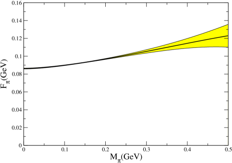
Figure 4: The plot on the left shows the $1\sigma$-band of the pion mass dependence of $F_{\pi}$. The plot on the right shows the dependence of $\xi$ on the pion mass, without including any uncertainty.

The pion mass dependence of $F_{\pi}$ is illustrated in Fig. 4 and is seen to be rather mild. This means that in the finite-volume condition (2) the numerical value on the r.h.s. (which was assigned using the physical pion mass) holds to a good approximation also for substantially heavier pions – the increase of $F_{\pi}$ with the pion mass is too mild to matter in this respect. In our numerical studies of the CHPT formulae we restrict ourselves to $L\!\geq\!1.5\,\mathrm{fm}$ and actually expect that this bound might already be too low with respect to the condition (2). Let us remark that the same bound has to be respected even if one works in the $\epsilon$–regime (4) and wants to compare to CHPT formulae: in this regime one must still have a relatively large volume and is consequently forced to use tiny – smaller than physical – quark masses.

By contrast, the parameter $\xi$ remains small even for pion masses of about half a GeV, as is shown on the right-hand side of Fig. 4. In our numerical analysis we will use $\xi$ exactly as given in this figure and ignore the uncertainties of this “computed” $\xi$ (shown only in the plot on the left-hand side of Fig. 4) since, as explained above, by measuring $F_{\pi}(L)$ one can determine $\xi$ iteratively from the lattice data. We do, however, determine the uncertainty of the coefficients $I_{2m}$ in the series (22), and for that aim we use the correlation matrix among the input parameters which can be obtained from Ref. [10]. The numerical values and the details of the analysis are given in Appendix C.

3.2 Finite volume effects in the pion mass

We are now in a position to evaluate the Lüscher formula (22) for the relative mass shift $R_{M}(M_{\pi},L)$. Before doing so, we find it instructive to have a look at the product

$$F({\rm i}y)\;e^{-\sqrt{M_{\pi}^{2}+y}\;L}$$ (31)

which is the integrand in the Lüscher formula (15).

Figure 5: The integrand $I(y)=e^{-\sqrt{M_{\pi}^{2}+y^{2}}\,L}\,F(\mathrm{i}y)$ with LO, NLO, NNLO input from CHPT. Note the change in scale in the lower panel.

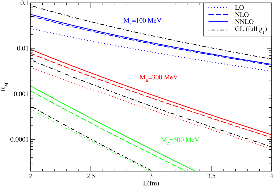
We have plotted this integrand in Fig. 5 for different values of $M_{\pi}$ and $L$, evaluated at LO, NLO and NNLO in the chiral expansion. Since the calculation is based on CHPT and the integration variable $y$ has the dimension of a mass, the integrand must tend to zero sufficiently fast beyond $O(100)\,\mathrm{MeV}$ – otherwise the outcome of the calculation cannot be trusted. This criterion results in a clear veto against too small box sizes (around $\sim\!1\,\mathrm{fm}$). By the absolute amount, the two integrands are close to each other whenever the pion is light and the box is sufficiently large. However, in the whole range of $M_{\pi}$ and $L$ shown in the graphs, the relative difference between the LO and the NLO integrand is substantial. The reason is that at LO the function $F(\nu)$ is a constant ($F_{2}$ can depend at most linearly on $\nu$, and since it has to be even in $\nu$ it can only be a constant): the energy dependence of the forward scattering amplitude – in particular the one dictated by the unitarity cuts – appears only at NLO. The difference between LO and NLO is therefore not very useful in judging the convergence of the chiral series, which should rather be evaluated by comparing NLO and NNLO. The plots in Fig. 5 show that even for $M_{\pi}=500$ MeV the correction in going from NLO to NNLO is not unacceptably large. Note that in the graphs in Fig. 5 the product $M_{\pi}L$ ranges from about 1 (top left) to 10 (bottom right): in the former case the product is too small for the asymptotic formula (15) to apply – we will confirm this below, by comparing this result to the one obtained with one-loop CHPT in finite volume, eq. (8).

Figure 6: The relative mass shift $R_{M}(M_{\pi},L)$ versus $L$ for a few values of the (infinite volume) mass $M_{\pi}$. In addition, the full 1-loop result (8) by Gasser and Leutwyler is included.

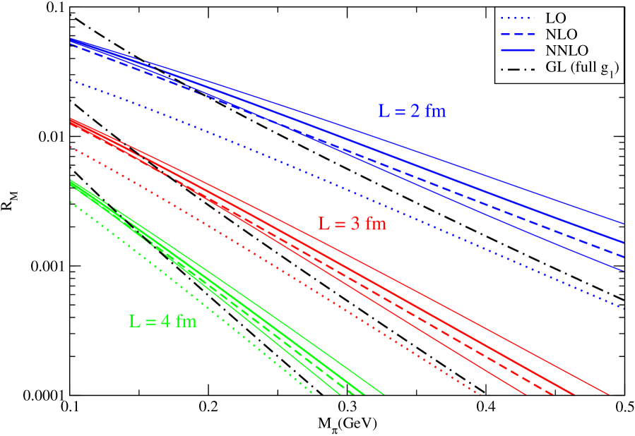
Figure 7: The relative mass shift $R_{M}(M_{\pi},L)$ versus $M_{\pi}$ for a few values of the box length $L$. The thin lines around the NNLO curves represent the corresponding uncertainties. For comparison, the full one-loop result (8) of Gasser and Leutwyler is included.

The relative mass shift $R_{M}(M_{\pi},L)$ calculated with the Lüscher formula (15, 22) is plotted in Fig. 6 as a function of $L$ for different values of $M_{\pi}$ and in Fig. 7 as a function of $M_{\pi}$ for selected values of $L$. In the latter figure we also show the uncertainty coming from the LEC – as expected the band grows with the pion mass. These figures show that the chiral expansion converges nicely for very light pions ($M_{\pi}\!=\!100$ MeV) and more slowly, but still satisfactorily for heavier pions. For light pions, however, the comparison between the full one-loop CHPT calculation and Lüscher’s formula (evaluated with the LO forward scattering amplitude) shows that the leading exponential behavior is not numerically dominating, even for volumes as large as $L\!=\!4$ fm (where $M_{\pi}L\!\sim\!2$ for the lightest pion considered). Here, the use of Lüscher’s formula is not justified, and one should rather rely on the full one-loop result in CHPT in finite volume. On the other hand, the fact that the NLO correction in Lüscher’s formula is rather large indicates that even the full one-loop result does not give a reliable answer. In such cases (e.g. when one will be able to simulate 200 MeV pions in a 2 fm volume) one would need a full two-loop calculation of the pion mass in CHPT in finite volume in order to reliably estimate the finite size corrections.

For heavier pion masses the higher exponentials which are neglected in Lüscher’s formula are less important and one is entitled to fully rely on this convenient formula. We find that for masses above 200 MeV and $L\geq 2$ fm the finite size effects are at most of the order of a few percent. We stress that in this range of masses and volumes our evaluation of the finite size effects is reliable because we are able to check both the convergence of the chiral expansion and that of the large volume expansion of Lüscher. For $M_{\pi}L\!\simeq\!4$ and $L\!\simeq\!4\,\mathrm{fm}$ or larger the predicted shift is below $0.1\%$: in such cases we may conclude that for all practical purposes the mass obtained on the lattice coincides numerically with the infinite-volume one. Mass shifts of the order of $1\%$ are predicted only for $M_{\pi}\simeq 200\div 300\,\mathrm{MeV}$, $L\simeq 2\div 2.5\,\mathrm{fm})$. This is the region where precision tests of lattice QCD calculations (we stress again that our calculation applies only to full QCD) will need the application of such corrections.

	$1.5\,\mathrm{fm}$	$2.0\,\mathrm{fm}$	$2.5\,\mathrm{fm}$	$3.0\,\mathrm{fm}$	$3.5\,\mathrm{fm}$	$4.0\,\mathrm{fm}$
$100\,\mathrm{MeV}$	$0.58\times 10^{-1}$	$2.73\times 10^{-2}$	$1.46\times 10^{-2}$	$0.83\times 10^{-2}$	$5.02\times 10^{-3}$	$3.13\times 10^{-3}$
	$1.35(3)$	$5.15(14)$	$2.41(7)$	$1.26(4)$	$7.15(24)$	$4.27(15)$
	$1.50(2)$	$5.60(14)$	$2.58(8)$	$1.34(5)$	$7.51(29)$	$4.45(18)$
	$2.39$	$8.74$	$3.85$	$1.91$	$10.2$	$5.81$
	$3.31$	$11.6$	$4.97$	$2.41$	$12.7$	$7.13$
$200\,\mathrm{MeV}$	$2.87\times 10^{-2}$	$1.08\times 10^{-2}$	$0.45\times 10^{-2}$	$2.04\times 10^{-3}$	$0.96\times 10^{-3}$	$0.47\times 10^{-3}$
	$6.22(47)$	$2.03(18)$	$0.78(8)$	$3.31(34)$	$1.50(16)$	$0.71(8)$
	$7.61(73)$	$2.39(27)$	$0.90(12)$	$3.74(52)$	$1.67(24)$	$0.78(12)$
	$6.56$	$2.00$	$0.73$	$2.95$	$1.29$	$0.59$
	$11.3$	$3.31$	$1.17$	$4.65$	$2.00$	$0.91$
$300\,\mathrm{MeV}$	$1.31\times 10^{-2}$	$0.39\times 10^{-2}$	$1.27\times 10^{-3}$	$0.45\times 10^{-3}$	$1.64\times 10^{-4}$	$0.62\times 10^{-4}$
	$2.87(41)$	$0.78(12)$	$2.42(41)$	$0.82(14)$	$2.93(53)$	$1.09(20)$
	$3.65(77)$	$0.95(22)$	$2.89(72)$	$0.96(25)$	$3.41(92)$	$1.26(35)$
	$2.25$	$0.56$	$1.65$	$0.54$	$1.88$	$0.69$
	$4.59$	$1.12$	$3.27$	$1.05$	$3.65$	$1.32$
$400\,\mathrm{MeV}$	$0.58\times 10^{-2}$	$0.13\times 10^{-2}$	$0.34\times 10^{-3}$	$0.94\times 10^{-4}$	$0.27\times 10^{-4}$	$0.79\times 10^{-5}$
	$1.35(28)$	$0.30(6)$	$0.74(17)$	$1.98(46)$	$0.56(13)$	$1.64(39)$
	$1.75(55)$	$0.37(12)$	$0.91(32)$	$2.41(86)$	$0.67(25)$	$1.96(73)$
	$0.85$	$0.17$	$0.40$	$1.03$	$0.29$	$0.83$
	$2.01$	$0.41$	$0.97$	$2.50$	$0.69$	$1.99$
$500\,\mathrm{MeV}$	$0.26\times 10^{-2}$	$0.47\times 10^{-3}$	$0.09\times 10^{-3}$	$0.20\times 10^{-4}$	$0.44\times 10^{-5}$	$0.10\times 10^{-5}$
	$0.66(17)$	$1.16(31)$	$0.23(6)$	$0.48(13)$	$1.07(29)$	$0.24(7)$
	$0.87(34)$	$1.50(60)$	$0.29(12)$	$0.61(26)$	$1.34(57)$	$0.31(13)$
	$0.34$	$0.54$	$0.10$	$0.21$	$0.45$	$0.10$
	$0.95$	$1.58$	$0.30$	$0.62$	$1.35$	$0.31$

Table 2: The relative finite size effect $R_{M}(M_{\pi},L)$ for selected values of $M_{\pi}$ and $L$. In each cell we give the result of the Lüscher formula (15) with the forward amplitude at LO, NLO and NNLO accuracy from CHPT. The fourth entry gives the GL result (8, 11) and the last one contains the full one-loop result shifted by the difference between the NNLO and the LO Lüscher formula – this, we believe, is a reasonable estimate of the total effect. The power of ten given in the first entry of the cell applies to all other entries. Note that the first column is very likely in conflict with the condition (2). Note, finally, that the GL result (9, 11) for the relative shift of $F_{\pi}$ is $(-4)$ times the fourth entry (for $N_{\!f\,}\!=\!2$).

Our numerical findings are summarized in Tab. 2, where we give for selected values of $M_{\pi}$ and $L$ the relative mass shift $R_{M}$ computed via the Lüscher formula (15, 22) with LO, NLO and NNLO input from CHPT. For comparison, we give the full one-loop result without large $L$ expansion (12, 14), due to Gasser and Leutwyler [2]. We have also combined the two results by adding to the NNLO Lüscher formula the series of large-$L$ suppressed exponentials which appears in the full one-loop result but not in Lüscher’s formula. This last figure is our best estimate of the total finite-size correction, but a sizable difference between this and the NNLO Lüscher result signals the presence of large uncertainties. In such cases (as we have argued above) a full two-loop evaluation of these corrections would presumably settle their value.

Note that in the first column of Tab. 2 we give the finite size effects for $L=1.5$ fm, although for such small volumes we are very likely already in conflict with (2), and are therefore outside the region of applicability of CHPT. We include this column in the hope that future high-precision lattice data in the regime $1.5\,\mathrm{fm}\!<\!L\!<\!2\,\mathrm{fm}$ might pinpoint what eqn. (2) means quantitatively.

4 Summary and Discussion

Making all the necessary extrapolations for lattice QCD calculations (lattice spacing to zero, quark masses to their physical value and volume to infinity) at the same time would be enormously expensive in terms of computer time and is practically unfeasible. Wherever possible one should try to use analytical methods as an aid. As far as the finite-volume effects are concerned, the necessary theoretical tools to control these artifacts have been developed in the eighties by Lüscher [8] and by Gasser and Leutwyler [2, 4].

Recent progress on the side of lattice calculations make now this issue of concrete relevance, and gave us the motivation to make a thorough numerical study of the finite size effects on the pion mass. In order to do so we have explicitly evaluated the Lüscher formula using as input the forward scattering amplitude evaluated at leading, next-to-leading and next-to-next-to-leading order in two-flavor CHPT. Pushing the chiral expansion to such a high order has shown to be absolutely essential in order to obtain good control on the convergence of the chiral series: for a wide range of pion masses and lattice volumes we find that the we can evaluate these corrections reliably. As shown first by Lüscher, these corrections vanish exponentially with $M_{\pi}L$ and are therefore negligible for sufficiently large masses and/or volumes. We have determined the regions where these corrections are important for precision calculations. Our numerical results are given in Figs. 6, 7 and in Table 2 – these are the main results of this paper.

If $M_{\pi}L$ is not very large, keeping only the leading exponential in the large volume expansion, as is the case in Lüscher’s formula (15), may not be accurate enough. In such cases one can take into account the whole series of exponentials by working with CHPT in finite volume. One-loop expressions for the pion mass and decay constant are available in the literature [2] and, in numerical form, in our Table 2, and we have used them to estimate numerically for which values of $M_{\pi}L$ is Lüscher’s formula not enough accurate. For such situations, it is at the moment difficult to estimate the size of finite-volume effects, and a full two-loop calculation in CHPT in finite volume seems the only viable way to do it reliably.

A: The coefficients $\bar{b}_{1},\,\ldots\,,\bar{b}_{6}$

For convenience we provide in this appendix the explicit expressions for the effective coupling constants $\bar{b}_{1},\ldots,\bar{b}_{6}$ which appear in the $\pi\pi$ scattering amplitude up to order $p^{6}$ [9, 10] in the split convention (24):

$$\bar{b}_{1}^{0} = -\frac{7}{6}\tilde{L}+\frac{4}{3}\tilde{\ell}_{1}-\frac{1}{2}\tilde{\ell}_{3}-2\,\tilde{\ell}_{4}+\frac{13}{18}$$

$$\bar{b}_{1}^{1} = -\frac{49}{6}\tilde{L}^{2}+\Big{\{}-\frac{4}{9}\tilde{\ell}_{1}-\frac{56}{9}\tilde{\ell}_{2}-\tilde{\ell}_{3}-\frac{26}{3}\tilde{\ell}_{4}-\frac{47}{108}\Big{\}}\tilde{L}+\frac{16}{3}\tilde{\ell}_{1}\tilde{\ell}_{4}-\frac{1}{2}\tilde{\ell}_{3}^{\;2}-3\,\tilde{\ell}_{3}\tilde{\ell}_{4}-5\,\tilde{\ell}_{4}^{\;2}$$

$$+\frac{28}{27}\tilde{\ell}_{1}+\frac{80}{27}\tilde{\ell}_{2}-\frac{15}{4}\tilde{\ell}_{3}+\frac{26}{9}\tilde{\ell}_{4}-\frac{34\pi^{2}}{27}+\frac{3509}{1296}+\tilde{r}_{1}$$

$$\bar{b}_{2}^{0} = \frac{2}{3}\tilde{L}-\frac{4}{3}\tilde{\ell}_{1}+2\,\tilde{\ell}_{4}-\frac{2}{9}$$

$$\bar{b}_{2}^{1} = \frac{431}{36}\tilde{L}^{2}+\Big{\{}6\,\tilde{\ell}_{1}+\frac{124}{9}\tilde{\ell}_{2}-\frac{5}{2}\tilde{\ell}_{3}+\frac{20}{3}\tilde{\ell}_{4}+\frac{203}{54}\Big{\}}\tilde{L}-\frac{16}{3}\tilde{\ell}_{1}\tilde{\ell}_{4}+\tilde{\ell}_{3}\tilde{\ell}_{4}+5\,\tilde{\ell}_{4}^{\;2}$$

$$-4\,\tilde{\ell}_{1}-\frac{166}{27}\tilde{\ell}_{2}+\frac{9}{2}\tilde{\ell}_{3}-\frac{8}{9}\tilde{\ell}_{4}+\frac{317\pi^{2}}{216}-\frac{1789}{432}+\tilde{r}_{2}$$

$$\bar{b}_{3}^{0} = \frac{1}{2}\tilde{L}+\frac{1}{3}\tilde{\ell}_{1}+\frac{1}{6}\tilde{\ell}_{2}-\frac{7}{12}$$

$$\bar{b}_{3}^{1} = -\frac{40}{9}\tilde{L}^{2}+\Big{\{}-\frac{38}{9}\tilde{\ell}_{1}-\frac{20}{3}\tilde{\ell}_{2}+2\,\tilde{\ell}_{4}+\frac{365}{216}\Big{\}}\tilde{L}+\frac{4}{3}\tilde{\ell}_{1}\tilde{\ell}_{4}+\frac{2}{3}\tilde{\ell}_{2}\tilde{\ell}_{4}$$

$$+\frac{89}{27}\tilde{\ell}_{1}+\frac{38}{9}\tilde{\ell}_{2}-\frac{7}{3}\tilde{\ell}_{4}-\frac{311\pi^{2}}{432}+\frac{7063}{864}+\tilde{r}_{3}$$

$$\bar{b}_{4}^{0} = \frac{1}{6}\tilde{L}+\frac{1}{6}\tilde{\ell}_{2}-\frac{5}{36}$$

$$\bar{b}_{4}^{1} = \frac{5}{6}\tilde{L}^{2}+\Big{\{}\frac{1}{9}\tilde{\ell}_{1}+\frac{8}{9}\tilde{\ell}_{2}+\frac{2}{3}\tilde{\ell}_{4}-\frac{47}{216}\Big{\}}\tilde{L}+\frac{2}{3}\tilde{\ell}_{2}\tilde{\ell}_{4}$$

$$+\frac{5}{27}\tilde{\ell}_{1}+\frac{4}{27}\tilde{\ell}_{2}-\frac{5}{9}\tilde{\ell}_{4}+\frac{17\pi^{2}}{216}+\frac{1655}{2592}+\tilde{r}_{4}$$

$$\bar{b}_{5} = \frac{85}{72}\tilde{L}^{2}+\Big{\{}\frac{7}{8}\tilde{\ell}_{1}+\frac{107}{72}\tilde{\ell}_{2}-\frac{625}{288}\Big{\}}\tilde{L}-\frac{31}{36}\tilde{\ell}_{1}-\frac{145}{108}\tilde{\ell}_{2}+\frac{7\pi^{2}}{54}-\frac{66029}{20736}+\tilde{r}_{5}$$

$$\bar{b}_{6} = \frac{5}{24}\tilde{L}^{2}+\Big{\{}\frac{5}{72}\tilde{\ell}_{1}+\frac{25}{72}\tilde{\ell}_{2}-\frac{257}{864}\Big{\}}\tilde{L}-\frac{7}{108}\tilde{\ell}_{1}-\frac{35}{108}\tilde{\ell}_{2}+\frac{\pi^{2}}{27}-\frac{11375}{20736}+\tilde{r}_{6}$$ (32)

where

$$\tilde{\ell}_{i}\equiv\log{\Lambda_{i}^{2}\over\mu^{2}}\;\;,\quad\tilde{r}_{i}=N^{2}r_{i}^{r}(\mu)\;\;,\quad\tilde{L}=\log{\mu^{2}\over M_{\pi}^{2}}\;\;.$$ (33)

Note that the quark masses exclusively enter through $\xi$ and $\tilde{L}$; the remaining quantities are independent thereof.

B: The functions $K_{i}^{\pi\pi}$

The functions $K_{i}^{\pi\pi}(x)$, $i=0,\ldots,4$ have been introduced in [9], and we reproduce them here for convenience. With

$$z=1-\frac{4}{x}\qquad\mathrm{and}\qquad{h}(x)=\frac{1}{N\sqrt{z}}\log\frac{\sqrt{z}-1}{\sqrt{z}+1}\;,$$

they read

$$K_{0}^{\pi\pi}(x) = {z\over N}h(x)+{2\over N^{2}}\qquad\Big{[}\;=\;{1\over N}\bar{J}\;\Big{]}$$

$$K_{1}^{\pi\pi}(x) = zh^{2}(x)$$

$$K_{2}^{\pi\pi}(x) = z^{2}h^{2}(x)-{4\over N^{2}}$$

$$K_{3}^{\pi\pi}(x) = {Nz\over x}h^{3}(x)+{\pi^{2}\over Nx}h(x)-{\pi^{2}\over 2N^{2}}$$

$$K_{4}^{\pi\pi}(x) = {1\over xz}\left[K_{0}^{\pi\pi}(x)+{1\over 2}K_{1}^{\pi\pi}(x)+{1\over 3}K_{3}^{\pi\pi}(x)+{(\pi^{2}-6)x\over 12N^{2}}\right]\;.$$

C: Evaluation of the uncertainties

In order to quantify the uncertainty of the $I_{2m}$ in (22), we need to know the correlation matrix among the LEC involved and the partial derivatives of the $I_{2m}$ w.r.t the LEC.

The correlation matrix $C_{ij}$ among our ten input parameters is given in Tab. 3. It has been obtained from Ref. [10], which represents so far the best determination of the LEC appearing in the $\pi\pi$ scattering amplitude. We remark that some of our input parameters were also used as input in [10] and therefore are statistically independent – this is seen in Tab. 3 where some of the off-diagonal matrix elements are zero.

Combining (25) and (32) one finds

$${\partial I_{4}\over\partial\tilde{\ell}_{1}}=4B^{0}-{8\over 3}B^{2}\;,\quad{\partial I_{4}\over\partial\tilde{\ell}_{2}}={8\over 3}B^{0}-{32\over 3}B^{2}\;,\quad{\partial I_{4}\over\partial\tilde{\ell}_{3}}=-{5\over 2}B^{0}\;,\quad{\partial I_{4}\over\partial\tilde{\ell}_{4}}=-2B^{0}$$ (34)

and

$${\partial I_{6}\over\partial\tilde{\ell}_{1}} = \Big{(}4\tilde{L}+16\tilde{\ell}_{4}+{20\over 9}\Big{)}B^{0}+\Big{(}-{40\over 3}\tilde{L}-{32\over 3}\tilde{\ell}_{4}+{32\over 9}\Big{)}B^{2}-8R_{0}^{2}+{16\over 3}R_{0}^{3}$$

$${\partial I_{6}\over\partial\tilde{\ell}_{2}} = \Big{(}{32\over 3}\tilde{\ell}_{4}+{64\over 9}\tilde{L}-{40\over 27}\Big{)}B^{0}+\Big{(}-{560\over 9}\tilde{L}-{128\over 3}\tilde{\ell}_{4}+{464\over 27}\Big{)}B^{2}$$

$$+{80\over 9}R_{0}^{0}-{80\over 9}R_{0}^{1}-{128\over 9}R_{0}^{2}-{16\over 3}R_{0}^{3}$$

$${\partial I_{6}\over\partial\tilde{\ell}_{3}} = \Big{(}-15\tilde{L}-5\tilde{\ell}_{3}-11\tilde{\ell}_{4}-{3\over 4}\Big{)}B^{0}-5R_{0}^{0}$$

$${\partial I_{6}\over\partial\tilde{\ell}_{4}} = \Big{(}{14\over 3}\tilde{L}+16\tilde{\ell}_{1}+{32\over 3}\tilde{\ell}_{2}-11\tilde{\ell}_{3}-10\tilde{\ell}_{4}-{110\over 9}\Big{)}B^{0}$$

$$+\Big{(}-{160\over 3}\tilde{L}-{32\over 3}\tilde{\ell}_{1}-{128\over 3}\tilde{\ell}_{2}+{448\over 9}\Big{)}B^{2}+{52\over 3}R_{0}^{0}-{64\over 3}R_{0}^{1}-{160\over 3}R_{0}^{2}$$

$${\partial I_{6}\over\partial\tilde{r}_{1}} = 5B^{0}(\lambda)$$

$${\partial I_{6}\over\partial\tilde{r}_{2}} = 4B^{0}(\lambda)$$

$${\partial I_{6}\over\partial\tilde{r}_{3}} = 8B^{0}(\lambda)-8B^{2}(\lambda)$$

$${\partial I_{6}\over\partial\tilde{r}_{4}} = 8B^{0}(\lambda)-56B^{2}(\lambda)$$

$${\partial I_{6}\over\partial\tilde{r}_{5}} = 16B^{0}(\lambda)-48B^{2}(\lambda)$$

$${\partial I_{6}\over\partial\tilde{r}_{6}} = 16B^{0}(\lambda)+16B^{2}(\lambda)\;.$$ (35)

These two vectors are then used to sandwich the correlation matrix of our input parameters. With $\vec{x}\equiv\{\tilde{\ell}_{1},\ldots,\tilde{\ell}_{4},\tilde{r}_{1},\ldots,\tilde{r}_{6}\}$, the resulting uncertainty is

$$\Delta R_{M}=\xi^{2}\sqrt{\sum_{i,j=1}^{10}\Big{(}{\partial I_{4}\over\partial x_{i}}+\xi{\partial I_{6}\over\partial x_{i}}\Big{)}\,C_{ij}\,\Big{(}{\partial I_{4}\over\partial x_{j}}+\xi{\partial I_{6}\over\partial x_{j}}\Big{)}}\;,$$ (36)

where $\partial I_{4}/\partial x_{i}$ is zero for $i>4$, and the rationale for omitting the uncertainty in our evaluation of $\xi$ has been explained in the text.

	$\tilde{\ell}_{1}$	$\tilde{\ell}_{2}$	$\tilde{\ell}_{3}$	$\tilde{\ell}_{4}$	$\tilde{r}_{1}$	$\tilde{r}_{2}$	$\tilde{r}_{3}$	$\tilde{r}_{4}$	$\tilde{r}_{5}$	$\tilde{r}_{6}$
$\tilde{\ell}_{1}$	$3.5\,10^{-1}$	$-3.3\,10^{-2}$	$-3.0\,10^{-2}$	$6.7\,10^{-2}$	$-8.8\,10^{-5}$	$1.7\,10^{-2}$	$-1.2$	$-2.1\,10^{-1}$	$-5.4\,10^{-1}$	$-3.7\,10^{-2}$
$\tilde{\ell}_{2}$		$1.2\,10^{-2}$	$-3.0\,10^{-3}$	$-7.2\,10^{-3}$	$7.2\,10^{-6}$	$3.7\,10^{-3}$	$9.8\,10^{-2}$	$-3.9\,10^{-1}$	$1.1\,10^{-2}$	$-4.6\,10^{-3}$
$\tilde{\ell}_{3}$			$5.8$	$-5.5\,10^{-2}$	$-$	$-$	$-$	$-$	$-3.3\,10^{-2}$	$7.0\,10^{-4}$
$\tilde{\ell}_{4}$				$4.8\,10^{-2}$	$-8.6\,10^{-6}$	$2.3\,10^{-3}$	$-1.2\,10^{-1}$	$-7.4\,10^{-2}$	$-9.1\,10^{-2}$	$-2.2\,10^{-3}$
$\tilde{r}_{1}$					$2.3$	$-$	$-$	$-$	$4.8\,10^{-4}$	$-5.7\,10^{-5}$
$\tilde{r}_{2}$						$10$	$-$	$-$	$-2.1\,10^{-2}$	$-5.8\,10^{-4}$
$\tilde{r}_{3}$							$18$	$-$	$2.3$	$1.6\,10^{-1}$
$\tilde{r}_{4}$								$6.3$	$1.9$	$3.7\,10^{-1}$
$\tilde{r}_{5}$									$1.1$	$9.2\,10^{-2}$
$\tilde{r}_{6}$										$1.1\,10^{-2}$

Table 3: The correlation matrix of our 10 input parameters.

References

• [1] J. Gasser and H. Leutwyler, Annals Phys. 158, 142 (1984).
• [2] J. Gasser and H. Leutwyler, Phys. Lett. B 184 83 (1987).
• [3] H. Leutwyler, Phys. Lett. B 189 197 (1987).
• [4] J. Gasser and H. Leutwyler, Nucl. Phys. B 307 763 (1988).
• [5] H. Neuberger, Phys. Rev. Lett. 60, 889 (1988). H. Neuberger, Nucl. Phys. B 300, 180 (1988). P. Hasenfratz and H. Leutwyler, Nucl. Phys. B 343 241 (1990). F.C. Hansen, Nucl. Phys. B 345 685 (1990).
• [6] A. Hasenfratz et al., Nucl. Phys. B 356 332 (1991). P.H. Damgaard, M.C. Diamantini, P. Hernandez and K. Jansen, Nucl. Phys. B 629 445 (2002) [hep-lat/0112016].
• [7] G. Colangelo, S. Dürr and R. Sommer, Nucl. Phys. Proc. Suppl.  119, 254 (2003) [hep-lat/0209110].
• [8] M. Lüscher, Commun. Math. Phys. 104, 177 (1986).
• [9] J. Bijnens, G. Colangelo, G. Ecker, J. Gasser and M. E. Sainio, Phys. Lett. B 374 210 (1996) [hep-ph/9511397]. Nucl. Phys. B 508 263 (1997) [Erratum-ibid. B 517 639 (1998)] [hep-ph/9707291].
• [10] G. Colangelo, J. Gasser and H. Leutwyler, Nucl. Phys. B 603, 125 (2001) [hep-ph/ 0103088].
• [11] J. Bijnens, G. Colangelo and P. Talavera, JHEP 9805, 014 (1998) [hep-ph/9805389].