Matter degrees of freedom and string breaking
in Abelian projected quenched SU(2) QCD

Abstract

In the Abelian projection the Yang–Mills theory contains Abelian gauge fields (diagonal degrees of freedom) and the Abelian matter fields (off-diagonal degrees) described by a complicated action. The matter fields are essential for the breaking of the adjoint string. We obtain numerically the effective action of the Abelian gauge and the Abelian matter fields in quenched $SU(2)$ QCD and show that the Abelian matter fields provide an essential contribution to the total action even in the infrared region. We also observe the breaking of an Abelian analog of the adjoint string using Abelian operators. We show that the adjoint string tension is dominated by the Abelian and the monopole contributions similarly to the case of the fundamental particles. We conclude that the adjoint string breaking can successfully be described in the Abelian projection formalism.

I Introduction

The mechanism of color confinement in QCD is one of the most important non–perturbative problems in the quantum field theory. One of the most promising approaches to this problem is based on the existence of the dual objects, called monopoles, which are condensed in the confinement phase. This approach – known as the dual superconductor hypothesis DualSuperconductor – is realized with the help of the so called Abelian projection 'tHooft:1981ht of $SU(N)$ color degrees of freedom to $U(1)^{N-1}$ degrees of freedom.

The model was shown to be quite successful in explanation of the confinement of the fundamental charges such as quarks (see, $e.g.$, reviews Reviews ). Abelian and monopole contributions to the inter–quark potential are dominant in the long-range region of quenched QCD suzuki90 ; ref:bali . An infrared effective monopole action has been derived in the continuum limit after a block–spin transformation of monopole currents shiba95 ; nakamura . It is a quantum perfect action described by the monopole currents. The condensation of the monopoles in the confinement phase was observed in various numerical approaches shiba95 ; MonopoleCondensation . In the language of the monopole currents the condensation implies the formation of the percolating cluster studied both numerically ref:MIP:clusters and analytically ref:Zakharov .

However, this mechanism has a serious problem even in quenched QCD. Although the ’t Hooft scenario describes the confinement of quarks correctly, this scenario predicts also the existence of the string tension for the adjoint charges (gluons) in the infrared region. On the other hand gluon charges must be screened at large distances due to the presence of the gluons in the QCD vacuum. This screening–confinement problem was extensively discussed in recent publications StringBreaking .

The problem of the screening of the adjoint charges in quenched $SU(N)$ QCD has also been discussed in Ref. greensite . The paper provides arguments that the relevant quantity in the confinement mechanism is not the Abelian monopoles but the $Z(N)$ center-vortices which can explain the screening problem ZNpicture . In our study we pursue a different approach based on the dual superconductor model.

Consider the screening in a confining Abelian model with the charge–two matter fields (take, for example, the Abelian Higgs model with the compact gauge fields). The presence of doubly charged matter fields screens the confining interaction between the external particles with opposite double charges. This happens due to the pair creation from the vacuum at certain separations between the external charges. As a result, the potential between the particles flattens at some distances. It should be stressed that the problem is not only to explain the flattening of the potential but also to show the linear behaviour of the potential in the intermediate region. On the other hand the charge–one external fields remain unscreened in this model. Namely, the potential is linearly rising at large distances.

The standard model of the dual superconductor in quenched QCD ignores the existence of the off-diagonal gluons. However, these gluons have a charge two with respect to the Abelian subgroup and they may explain the flattening of the inter–gluon potential which is usually studied with the help of the adjoint Wilson loop. On the other hand the introduction of the new degrees of freedom – the off-diagonal gluons – should not violate already achieved success of the explanation of the quark confinement in this model. Indeed, quarks have the charge one and doubly charged gluons can not screen them. These and related issues were discussed in Ref. SuzukiChernodub02 for quenched as well as for full $SU(N)$ QCD.

From the point of view of a realization of the (modified) dual superconductor scenario it seems that we have to keep all charge two Abelian Wilson loops in the effective action written by the Abelian link fields to reproduce the screening of charge two. Indeed, the theory in terms of the Abelian link fields or the Abelian monopole currents alone becomes highly non–local if we integrate out all off-diagonal gluon fields after an Abelian projection. Needless to say, such an Abelian effective action is useless. The same problem is more serious in the real full QCD, since a fundamental charge is also screened in this case.

The aim of this paper is to calculate numerically the effective action of quenched QCD within the Abelian projection formalism. Contrary to previous calculations of this kind we include also the doubly charged off-diagonal gluon fields into the effective action and we show that their contribution is essential and thus can not be neglected. We also calculate correlators of the adjoint Polyakov loops in the Abelian formalism and observe the screening of a properly defined potential between static adjoint sources.

The plan of the paper is the following. In Section II we discuss how the screening and confinement problem is solved qualitatively in the framework of Abelian dynamics. Section III is devoted to the investigation of the Abelian action for the Abelian gauge and matter fields obtained by the inverse Monte-Carlo method. In Section IV we discuss the potential between the adjoint ($Q=2$) charges within the Abelian projection formalism. We show numerically that properly defined Abelian potential shows screening of the $Q=2$ charges. Moreover, we observe the Abelian and the monopole dominance for the adjoint string tension. Our conclusions are presented in the last Section.

II String Breaking in Abelian Projected Theory

The partition function of the Abelian effective theory of quenched $SU(2)$ QCD in the infrared region may be approximated in the Villain–like form chernodub :

$$Z_{Q}[J]=\int\limits_{-\pi}^{\pi}{\cal D}\theta\sum_{n\in Z\!\!\!Z(c_{2})}e^{-\frac{1}{4\pi^{2}}((d\theta+2\pi n),\Delta D(d\theta+2\pi n))+iQ(\theta,J)}\,,$$ (1)

where $D$ is a differential operator

$$D\approx\bar{\alpha}+\bar{\beta}\Delta^{-1}+\bar{\gamma}\Delta\,.$$ (2)

This operator contains local self–interaction term, the Coulomb term described by the inverse Laplacian, $\Delta^{-1}$, and additional interactions between nearest neighbors. The coupling constants $\bar{\alpha}$, $\bar{\beta}$ and $\bar{\gamma}$ were calculated numerically in Ref. chernodub . To simplify notations we use the differential form formalism on the lattice DiffLattice .

The partition function (1) can be rewritten as a string model chernodub ,

$$Z_{Q}[J]\propto\sum_{\stackrel{{\scriptstyle\sigma\in Z\!\!\!Z(c_{2})}}{{\delta\sigma=QJ}}}e^{-\pi^{2}(\sigma,(\Delta D)^{-1}\sigma)}\,,$$ (3)

where we have neglected perimeter terms. This model does not contain the dynamical matter fields and therefore the string variable $\sigma$ is always closed on the external current $J$. Therefore there is no source for the string breaking in this model.

Now let us consider the off-diagonal gluons. The Wilson action of quenched $SU(2)$ QCD is

$$S=\frac{\beta}{2}\sum_{s,\mu,\nu}\,{\mathrm{Tr}}\,U_{\mu\nu}(s)\,,\quad U_{\mu\nu}(s)=U_{\mu}(s)U_{\nu}(s+\hat{\mu})U_{\mu}^{{\dagger}}(s+\hat{\nu})U_{\nu}^{{\dagger}}(s)\,,$$ (4)

where $U_{\mu}(s)$ is the $SU(2)$ gauge field.

It is convenient to parameterize the $SU(2)$ link variable $U_{\mu}(s)$ as $U_{\mu}(s)=c_{\mu}(s)u_{\mu}(s)$ where

$$c_{\mu}(s)=\left(\begin{array}[]{@{}cc@{}}\cos\phi_{\mu}(s)&i\sin\phi_{\mu}(s)e^{-i\varphi_{\mu}(s)}\\ i\sin\phi_{\mu}(s)e^{i\varphi_{\mu}(s)}&\cos\phi_{\mu}(s)\end{array}\right)\,,\quad u_{\mu}(s)=\left(\begin{array}[]{@{}cc@{}}e^{i\theta_{\mu}(s)}&0\\ 0&e^{-i\theta_{\mu}(s)}\end{array}\right)\,.$$ (8)

Here $\theta$, $\varphi$ and $\phi$ are independent variables defined in the regions $-\pi\leq\theta_{\mu}(s),\varphi_{\mu}(s)<\pi$ and $0\leq\phi_{\mu}(s)<\frac{\pi}{2}$. The field $\theta$ behaves as a $U(1)$ gauge field while the field $\varphi$ corresponds to the phase of the off–diagonal gluon field because under an Abelian gauge transformation,

$$\Omega^{\mathrm{Abel}}(s)={\mathrm{diag}(e^{i\alpha(s)},e^{-i\alpha(s)})}\,,$$ (9)

they behave as follows:

$$\theta_{\mu}(s)\to\theta_{\mu}(s)-\partial_{\mu}\alpha(s)\equiv\theta_{\mu}(s)+\alpha(s)-\alpha(s+\hat{\mu})\,,\quad\varphi_{\mu}(s)\to\varphi_{\mu}(s)+2\alpha(s)\,.$$ (10)

The variable $\phi_{\mu}(s)$ is not affected by the $U(1)$ gauge transformation. After an Abelian projection we can integrate this variable out without harming the $U(1)$ content of the model. In order to get an insight of possible forms of interactions between the Abelian gauge and Abelian matter fields we replace the averages of $\cos\phi_{\mu}(s)$ and $\sin\phi_{\mu}(s)$ by their mean values:

$$\cos\phi_{\mu}(s)\to\langle\cos\phi_{\mu}(s)\rangle\equiv c\,,\quad\sin\phi_{\mu}(s)\to\langle\sin\phi_{\mu}(s)\rangle\equiv s\,,$$ (11)

where $c$ and $s$ are functions of the $SU(2)$ coupling constant $\beta$.

As the Abelian projection, we use the Maximal Abelian gauge which is defined by a maximization of the functional,

$$R=\frac{1}{2}\sum_{s,\mu}{\rm Tr}\Big{(}\sigma_{3}\widetilde{U}_{\mu}(s)\sigma_{3}\widetilde{U}^{\dagger}_{\mu}(s)\Big{)}\equiv\sum_{s,\mu}(2\cos^{2}\phi_{\mu}(s)-1)\,,$$ (12)

with respect to the $SU(2)$ gauge transformations, $U_{\mu}(s)\to\widetilde{U}_{\mu}(s)=\Omega(s)U_{\mu}(s)\Omega^{\dagger}(s+\hat{\mu})$. The functional (12) is invariant under residual $U(1)$ gauge transformations (9). The local condition corresponding to maximization (12) can be written in the continuum limit as the differential equation $(\partial_{\mu}+igA_{\mu}^{3})(A_{\mu}^{1}-iA_{\mu}^{2})=0$.

The maximization of the functional (12) corresponds to the minimization of the $\phi$ variable. Thus the observation of Refs. suzukiNPBPS ; Chernodub:pw made for the mean values (11),

$$c\simeq 1\,,\quad s\ll c\,.$$ (13)

does not come as a surprise. These relations hold in a wide region of the coupling constant $\beta$.

Following Ref. Chernodub:pw we rewrite the action of the model (4) in terms of the variables $\theta$, $\varphi$ and $\phi$ with the help of the definitions (8). Applying Eq. (11) to the original action we get

$$\frac{1}{2}{\mathrm{Tr}}\,U_{\mu\nu}(s)=c^{4}\cos(\Theta_{\mu\nu}(s))-c^{2}s^{2}\cos(\Theta_{\mu\nu}(s)-H_{\mu\nu}(s)-C_{\mu\nu}(s))$$

$$-c^{2}s^{2}\cos(\Theta_{\mu\nu}(s)+H_{\nu\mu}(s)-C_{\mu\nu}(s))+c^{2}s^{2}\cos(\Theta_{\mu\nu}(s)+H_{\nu\mu}(s))$$ (14)

$$+c^{2}s^{2}\cos(\Theta_{\mu\nu}(s)-H_{\mu\nu}(s)+H_{\nu\mu}(s)-C_{\mu\nu}(s))+c^{2}s^{2}\cos(\Theta_{\mu\nu}(s)-H_{\mu\nu}(s))$$

$$+c^{2}s^{2}\cos(\Theta_{\mu\nu}(s)+C_{\mu\nu}(s))+s^{4}\cos(\Theta_{\mu\nu}(s)-H_{\mu\nu}(s)+H_{\nu\mu}(s)-2C_{\mu\nu}(s)),$$

where we have denoted the $U(1)$ gauge invariant variables as follows:

$$\Theta_{\mu\nu}(s) = \theta_{\mu}(s)+\theta_{\nu}(s+\hat{\mu})-\theta_{\mu}(s+\hat{\nu})-\theta_{\nu}(s)\,,$$ (15)

$$H_{\mu\nu}(s) = 2\theta_{\mu}(s)+\varphi_{\nu}(s)-\varphi_{\nu}(s+\hat{\mu})\,,$$ (16)

$$C_{\mu\nu}(s) = \varphi_{\mu}(s)-\varphi_{\nu}(s)\,.$$ (17)

The variable $\Theta$ is the $U(1)$ plaquette for the gauge field $\theta$, the variable $H$ describes the interaction of the matter field $\varphi$ with the gauge field $\theta$ and the variable $C$ corresponds to the self–interaction of the matter field. The validity of the mean field approximation based on a self–consistent substitution (11) is not known. When we perform the $\phi$ integration, we generally get an effective action in terms of $\Theta_{\mu\nu}$, $H_{\mu\nu}$ and $C_{\mu\nu}$. Below we use numerical method to find this effective action.

A few remarks about the action (14) are now in order. (i) From Eq. (13) one can immediately observe that the leading contribution to the action is provided by the first QED–like term depending on the variables $\theta$ only. The coupling between the gauge field $\theta$ and the matter field $\varphi$ is suppressed and the self–interaction of the matter field is suppressed even further. (ii) The action (14) should acquire corrections from the Faddeev–Popov determinant resulting from the fixing of the Maximal Abelian gauge. This determinant is an essentially non–local functional and the leading local terms were calculated in Ref.Chernodub:pw .

Let us assume for simplicity the following effective action:

$$S_{{\rm eff.}}=S^{(1)}(\theta)+S^{(2)}(\theta,\varphi)\,,\quad S^{(2)}(\theta,\varphi) = -F_{1}(H)-F_{2}(H^{\prime})-F_{3}(C)\,.$$ (18)

where we put $H=H_{\mu\nu}(s)$, $H^{\prime}=H_{\nu\mu}(s)$, $C=C_{\mu\nu}(s)$ and $F_{1}$, $F_{2}$, $F_{3}$ are periodic functions. Following Ref. SuzukiChernodub02 we rewrite the corresponding partition function $Z$ with the external source $J$ as follows:

$$Z_{Q}[J] = \int\limits_{-\pi}^{\pi}{\cal D}\theta{\cal D}\varphi\,e^{-S_{{\rm eff.}}+iQ(\theta,J)}=\int\limits_{-\pi}^{\pi}{\cal D}\theta{\cal D}\varphi\,\,e^{-S^{(1)}(\theta)-S^{(2)}(\theta,\varphi)+iQ(\theta,J)}$$ (19)

$$= \int\limits_{-\pi}^{\pi}{\cal D}\theta\hskip 2.84526pte^{-S^{(1)}(\theta)+iQ(\theta,J)}\left[\int\limits_{-\pi}^{\pi}{\cal D}\varphi\,e^{F_{1}(H)+F_{2}(H^{\prime})+F_{3}(C)}\right]\,.$$

The part in the square brackets can be expanded in the Fourier series,

$$[\cdots] = \int\limits_{-\pi}^{\pi}{\cal D}\varphi\sum_{\stackrel{{\scriptstyle n^{(i)}\in Z\!\!\!Z(c_{2})}}{{i=1,2,3}}}I_{1}(n^{(1)})\,I_{2}(n^{(2)})\,I_{3}(n^{(3)})\,e^{i(H,n^{(1)})+i(H^{\prime},n^{(2)})+i(C,n^{(3)})}\,.$$ (20)

where $n^{(i)}$, $i=1,2,3$ are integers and the lattice tensors $H$, $H^{\prime}$, $n^{(1)}$, $n^{(2)}$ sum only for $\mu>\nu$ because $H$, $H^{\prime}$ are not anti–symmetric contrary to $(C,n^{(3)})$.

Integrating over $\varphi$ and summing over $n^{(3)}$ one can rewrite Eq. (20) as follows:

$$[\cdots]=\sum_{\stackrel{{\scriptstyle j\in Z\!\!\!Z(c_{1})}}{{\delta j=0}}}w(j)\,e^{2i(\theta,j)}\,,$$ (21)

where $w(j)$ are certain weights for the closed current $j$ which is defined from the variables $n^{(1)}$ and $n^{(2)}$.

$$j_{\mu}(s)=\sum_{\nu(<\mu)}n_{\mu\nu}^{(1)}(s)+\sum_{\nu(>\mu)}n^{(2)}_{\nu\mu}(s)\,.$$ (22)

The general form of Eqs. (21) and (22) follows from the fact that the fields $\varphi$ are doubly charged and from the gauge invariance of the expression under the exponential function in Eq. (20). We also give a detailed derivation of Eqs. (21) and (22) in Appendix A.

To simplify further considerations let us rewrite the first term in Eq. (18) in the Villain form as in Eq. (1). Then we get for the partition function (19):

$$Z_{Q}[J]\!=\!\int\limits_{-\pi}^{\pi}\!{\cal D}\theta\!\!\!\sum_{n\in Z\!\!\!Z(c_{2})}\sum_{\stackrel{{\scriptstyle j\in Z\!\!\!Z(c_{1})}}{{\delta j=0}}}\!w(j)\,\exp\Bigl{\{}-\frac{1}{4\pi^{2}}((d\theta+2\pi n),\Delta D(d\theta+2\pi n))+i(\theta,2j+QJ)\Bigr{\}}\,.$$

Analogously to Eq. (3) we get the following model for the string variables dual to the gauge field $\theta$:

$$Z_{Q}[J]=\sum_{\stackrel{{\scriptstyle j\in{Z\!\!\!Z}(c_{1})}}{{\delta j=0}}}\sum_{\stackrel{{\scriptstyle\sigma\in{Z\!\!\!Z}(c_{2})}}{{\delta\sigma=2j+QJ}}}w(j)\,\exp\Bigl{\{}-\pi^{2}(\sigma,(\Delta D)^{-1}\sigma)\Bigr{\}}\,.$$ (23)

The string model (23) is different from the model (3) by the presence of the doubly charged currents representing the contribution of the off-diagonal gluons (the first sum in Eq. (23)). The second sum in this equation is over the integer valued string variable which has the dynamical current $j$ as its boundary.

If the external charge has a unit value, $Q=1$, then the dynamical current $j$ can not screen the external current $QJ$ and therefore the string always spans on the trajectories of the external currents, $\delta\sigma=2j+QJ\neq 0$. However, if the external current is doubly charged, $Q=2$, then there exists the dynamical current $j=-J$ such that $\delta\sigma=0$. This state breaks the string: when the distance between the external charges is large enough the state with $j=-J$ provides a dominant contribution to the partition function.

III Effective Action for Gauge and Matter fields

In this Section we calculate numerically the effective action for the Abelian gauge and the matter fields in quenched $SU(2)$ QCD. We have chosen a trial action in the form:

$$S_{\mathrm{eff}}(\theta,\varphi) = \alpha_{1}S_{1}(\theta)+\alpha_{2}S_{2}(\theta)+\alpha_{3}S_{3}(\theta)+\beta_{1}S_{4}(\theta,\varphi)\,,$$ (24)

where $\alpha_{i}$, $i=1,2,3$ and $\beta_{1}$ are the coupling constants to be determined numerically.

The functionals $S_{i}$, $i=1,2,3$ describe the action of the gauge field $\theta$,

$$S_{1} = -\sum_{s,\mu\neq\nu}[\cos\Theta_{\mu\nu}(s)]\,,$$ (25)

$$S_{2} = -\sum_{s,\mu\neq\nu}[\cos 2\Theta_{\mu\nu}(s)]\,,$$ (26)

$$S_{3} = +\sum_{s,\mu\neq\nu}[\sin\Theta_{\mu\nu}(s)\sin\Theta_{\mu\nu}(s+\hat{\mu})]\,,$$ (27)

where the plaquette variable $\Theta$ is given in Eq. (15). The action $S_{1}$ is the leading term in the Abelian action (14) corresponding to quenched $SU(2)$ QCD in the mean–field approximation. The parts $S_{2,3}$ are also included because they may arise naturally from the integration over $\phi$.

As an interaction term between the gauge, $\theta$, and the matter, $\varphi$, fields we adopt for simplicity

$$S_{4} = -\sum_{s,\mu\neq\nu}\Bigl{[}\cos(\Theta_{\mu\nu}(s)-H_{\mu\nu}(s))+\cos(\Theta_{\mu\nu}(s)+H_{\nu\mu}(s))\Bigr{]}\,,$$ (28)

where the plaquette variable $H$ is given in Eq. (16). We have not included other terms from Eq. (14) into the trial action because it turns out that the minimal form of the action (24) describes the numerical data with a good accuracy.

We have used the standard Monte–Carlo procedure to generate the gauge field configurations on the $32^{4}$ lattice. The $SU(2)$ coupling constant was chosen in the range $\beta=2.1\sim 2.7$. We have generated 100 configurations of the gauge field for each value of the coupling constant and then used the Simulated Annealing method ref:bali to fix the Maximal Abelian gauge. The couplings $\alpha_{i}$, $i=1,2,3$ and $\beta_{1}$ were determined by solving the Schwinger–Dyson equations ref:Okawa . We describe the details of this method in Appendix B. To make further improvement of our results towards the continuum limit we used also a blockspin transformation for the $SU(2)$ link variable $U_{\mu}(s)$: We apply the blockspin transformation to the link variable $U_{\mu}(s)$,

$$U^{\prime}_{\mu}(s^{\prime})=\frac{1}{N}\left(U_{\mu}(s)U_{\mu}(s+\hat{\mu})+\gamma\sum_{\nu(\neq\mu)}U_{\nu}(s)U_{\mu}(s+\hat{\nu})U_{\mu}(s+\hat{\mu}+\hat{\nu})U^{{\dagger}}_{\nu}(s+2\hat{\mu})\right)\,.$$ (29)

which is visually represented in Figure 1. Here $N\equiv N(U)$ is the normalization factor which is introduced to make the fat link belonging to the $SU(2)$ group. The weight parameter $\gamma$ was set to $\gamma=0.5$.

Figure 1: The visualization of the blockspin transformation, Eq. (29).

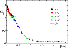
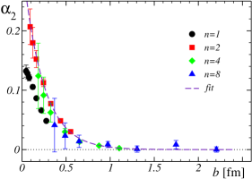
(a)	(b)
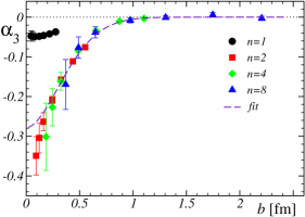
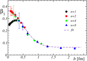
(c)	(d)

Figure 2: The parameters $\alpha_{i}$, $i=1,2,3$ and $\beta_{1}$ for different blocking steps $n$ $vs.$ the scale parameter $b$. The fits by Eq. (30) are shown by the dashed lines.

The couplings obtained in this way are depicted in Figures 2(a-d). The coupling $\alpha_{1}$ shows a perfect scaling since the coupling constant depends only on the physical length $b$, (and it does not depend on $n$ and $a$ separately). For the couplings $\alpha_{2}$, $\alpha_{3}$ and $\beta_{1}$ this feature does not work: the original data (no blockspin transformation, $n=1$) is quite different from the cases where the blockspin transformation was done ($n>1$) while the coupling constants with $n>1$ scale almost perfectly. One can make a conclusion that the original data corresponds to very small values of $b$ where the effective action takes more complicated form than (24).

In order to quantitatively characterize the dependence of the coupling constants on the scale factor $b$ we have fitted the data by a function

$$f(b)=C_{0}+C_{1}\exp\{-({b/b_{0})}^{\nu}\}\,,$$ (30)

where $C_{0,1}$, $\nu$ and $b_{0}$ are the fitting parameters. In our fits we have excluded the data without the blockspin transformation, $n=1$, for all coupling constants except for $\alpha_{1}$ case. The best fit curves are plotted in Figures 2 as the dashed lines, and the best fit parameters are shown in Table 1.

coupling	$C_{0}$	$C_{1}$	$b_{0}$, [fm]	$\nu$
$\alpha_{1}$	0.066(10)	1.20(2)	0.61(1)	2
$\alpha_{2}$	0	0.32(2)	0.231(7)	1
$\alpha_{3}$	0	-0.28(3)	0.46(3)	1.8(2)
$\beta_{1}$	0.064(5)	0.30(1)	0.69(2)	2

Table 1: The parameters for the exponential fits (30) of the couplings $\alpha_{i}$, $i=1,2,3$ and $\beta_{1}$.

We have found that in the case of $\alpha_{1}$ and $\beta_{1}$ the parameter $\nu$ is very close to two, and therefore in these fits we fixed this parameter, $\nu=2$. Similarly, we have also fixed $\nu=1$ for $\alpha_{2}$ and $C_{0}=0$ for $\alpha_{2,3}$. Note that the fit can not describe the coupling $\alpha_{1}$ accurately at small scales, $b\leqslant 0.2$ fm. A similar deviation can be found for the coupling $\alpha_{3}$. We expect that at small scales the Abelian action becomes much more complicated than the trial action (24,25,26,27,28) which we used to solve the Schwinger–Dyson equations. The small similar effect is observed for the effective monopole action obtained by the inverse Monte–Carlo methods chernodub .

The functional $S_{1}$, Eq. (25), makes the leading contribution to the action since the corresponding coupling, $\alpha_{1}$, is the largest. The actions $S_{2}$ and $S_{3}$, in addition to the expected action $S_{1}$, play an essential role at small scales since the corresponding couplings, $\alpha_{2}$ and $\alpha_{3}$, are non–vanishing. The action $S_{4}$, which describes the interaction of the matter fields with the gauge fields, has a non–vanishing coupling both at small and large scales similarly to $S_{1}$. Moreover, according to Table 1 the couplings $\alpha_{1}$ and $\beta_{1}$, corresponding to these parts of the total action, have relatively large lengths $b_{0}$ compared to the coupling constants $\alpha_{2}$ and $\alpha_{3}$. Thus, at large scales, $b\sqrt{\sigma}\gg 1$, the effective Abelian action for the $SU(2)$ gauge theory can be approximated as a sum of the QED–like action for the gauge field, $S_{1}(\theta)$, and the interaction term $S_{4}(\theta,\varphi)$.

We interpret the results, obtained in this Section as the manifestation of the Abelian dominance (non–vanishing dominant coupling $\alpha_{1}$) and the importance of the off-diagonal (matter) degrees of freedom (non–vanishing coupling $\beta_{1}$). The matter fields are essential for the breaking of the adjoint string. From the point of view of further analytical study the results of this Section are qualitative because in order to make a quantitative analytical predictions at a finite value of the scale $b$ we need much more terms in the trial action (24) than we have imposed. Indeed, in Ref. chernodub the monopole contribution to the string tension has been calculated using the effective monopole action. The monopole action was obtained numerically and it turns out that in order to get a correct analytical result for the string tension one should take into account not only the most local terms in the effective monopole action but also a series of the non–local terms. The situation with the effective action for the Abelian fields (24) should be similar to the case of the monopole action since these actions are related to each other chernodub . Nevertheless the adjoint string breaking can quantitatively be discussed within the numerical approach on the basis of the Maximal Abelian gauge fixing. This topic is discussed in the next Section.

IV $Q=2$ Potential from Polyakov Loops

The easiest way to observe numerically the string breaking effect is to consider the theory at finite temperature and define the potential with the help of the Polyakov loop correlators ref:PolyakovLoopOthers ; SuzukiChernodub02 :

$$\langle P(\vec{x})P^{{\dagger}}(\vec{y})\rangle = e^{-V(\vec{x}-\vec{y})/T}\,.$$ (31)

Here $T$ is temperature.

The adjoint Polyakov loop, $P_{1}$, is defined as follows:

$$P_{1}=\frac{1}{3}{\mathrm{Tr}}\,\left(\prod_{i\in{\cal C}}D_{1}[U_{i}]\right)=\frac{1}{3}(4p_{0}^{2}-1)\,,$$ (32)

where the color vector $p=p_{0}+i\vec{p}\cdot\vec{\sigma}$ defines the fundamental Polyakov loop, $P_{1/2}=1/2{\mathrm{Tr}}\,p$, $p=\prod_{i\in{\cal C}}U_{i}$, and ${\cal C}$ is the straight line parallel to the temperature direction. The adjoint Polyakov loop (32) contains the charged term, $Q=2$, and neutral term, $Q=0$:

$$P_{Q=2}=\frac{2}{3}(p_{0}^{2}-p_{3}^{2})\,,\quad P_{Q=0}=\frac{1}{3}(2p_{0}^{2}+2p_{3}^{2}-1)\,.$$ (33)

The Abelian dominance in the most general sense means that a non–Abelian observable can be calculated with a good accuracy with the help of the corresponding Abelian operator in a suitable Abelian projection. The Abelian dominance was first established for the tension of the chromoelectric string spanned between the fundamental sources suzuki90 . In this case the non–Abelian Wilson (or, Polyakov) loop was replaced by its Abelian counterpart.

However, in the case of the adjoint potential we immediately encounter a problem ref:greensite:caution : in the Abelian projection the $Q=2$ charged component of the Wilson loop shows the area law while the neutral $Q=0$ component is constant. Therefore, strictly speaking, the straightforward Abelian projection of the adjoint operators leads to the vanishing Abelian string tension. The simplest way to overcome this difficulty is to introduce the obvious prescription for the adjoint operators proposed originally in Ref. ref:poulis . Namely, one should disregard the $Q=0$ component of the Wilson loop operator and consider the $Q=2$ Abelian component of the Wilson loop as the Abelian analog of the full (non-Abelian) loop. In Ref. ref:poulis some numerical arguments in favor of the validity of this prescription were given. Below we follow this recipe and show that the string breaking effect can indeed be seen in the $Q=2$ Abelian and monopole components of the potential. Moreover, we have observed the Abelian and monopole dominance for the adjoint string tension.

After the Abelian projection the $Q=2$ component becomes

$$P_{Q=2}^{\rm ab}=\cos 2\vartheta_{\cal C}\,,\quad\vartheta_{\cal C}=\sum_{i\in{\cal C}}\theta_{i}\,.$$ (34)

where $\vartheta_{\cal C}$ enters the $Q=1$ Abelian Polyakov loop, $P^{\rm ab}_{1/2}=\cos\vartheta_{\cal C}$.

We calculate numerically the static potential between the adjoint particles using the Polyakov loop correlators (31). We use four types of the Polyakov loops: non-Abelian, Abelian, monopole and photon Polyakov loops,

$$P_{Q=2}=p_{0}^{2}-p_{3}^{2}\,,\quad P_{Q=2}^{\rm ab}=\cos 2\vartheta_{\cal C}\,,\quad P_{Q=2}^{\rm mon}=\cos 2\vartheta_{\cal C}^{\rm mon}\,,\quad P_{Q=2}^{\rm ph}=\cos 2\vartheta_{\cal C}^{\rm ph}\,,$$ (35)

respectively.

The functions $\vartheta_{\cal C}^{\rm mon}$ and $\vartheta_{\cal C}^{\rm ph}$ represent the contributions to the Polyakov loop coming from the monopole currents and the photon fields, respectively ref:bali ; suzuki90 :

$$\vartheta_{\cal C}^{\rm mon} = -\sum_{t}\sum_{\vec{x}^{\prime},t^{\prime}}D(\vec{x}-\vec{x}^{\prime},t-t^{\prime})\partial^{\prime}_{\mu}\bar{\Theta}_{\mu 4}(\vec{x}^{\prime},t^{\prime})\,,$$ (36)

$$\vartheta_{\cal C}^{\rm ph} = -2\pi\sum_{t}\sum_{\vec{x}^{\prime},t^{\prime}}D(\vec{x}-\vec{x}^{\prime},t-t^{\prime})\partial^{\prime}_{\mu}n_{\mu 4}(\vec{x}^{\prime},t^{\prime})\,,$$ (37)

where the variables $\bar{\Theta}\in(-\pi,\pi)$ and $n\in Z\!\!\!Z$ are extracted from the Abelian plaquette variable, $\Theta_{\mu\nu}(s)\equiv\theta_{\mu}(s)+\theta_{\nu}(s+\hat{\mu})-\theta_{\mu}(s+\hat{\nu})-\theta_{\nu}(s)=\bar{\Theta}_{\mu\nu}(s)+2\pi n_{\mu\nu}(s)$. $D(s)$ is the inverse Laplacian, $\partial^{\prime}_{\mu}\partial_{\mu}D(s)=-\delta_{0,s}$.

We numerically measured the potential between the static adjoint sources on the $16^{3}\times 4$ lattice at $\beta=2.2$ (confinement phase) using 2000 configurations. The Abelian, monopole and the photon components of the potential were measured in the Maximal Abelian gauge. In order to reduce the statistical errors in our calculations of the potentials we have applied the Hypercubic Blocking ref:HCB procedure to ensembles of the non–Abelian, Abelian and photon gauge fields. We have not applied the blocking to the monopole contribution of the potential because in this particular case the blocking makes the data noisier. The Hypercubic Blocking method is briefly described in Appendix C.

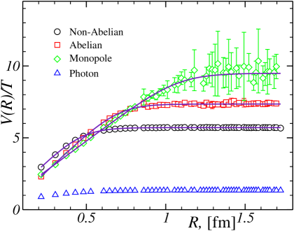
Figure 3: The potential between adjoint static sources and the Abelian, the monopole and the photon contributions to it. The fits by the function (38) are shown by the solid lines.

We present the numerical results in Figure 3. One can clearly see that all potentials become flat in the infrared region clearly indicating the presence of the string breaking. The non-Abelian potential as well as the Abelian and the monopole contributions contain the linear pieces at small enough distances while the photon contribution to the potential does not contain a linear part. These observations are in a qualitative agreement with the Abelian (monopole) dominance hypothesis suzuki90 .

To make a quantitative characterization of the potentials we fit our data by a function

$$\exp\Bigl{\{}-\frac{V^{\mathrm{fit}}(R)}{T}\Bigr{\}}=\exp\Bigl{\{}-\frac{V_{0}+2m}{T}\Bigr{\}}+\exp\Bigl{\{}-\frac{V_{0}+V_{\mathrm{str}}(R)}{T}\Bigr{\}}\,,$$ (38)

where we have chosen the string potential in the simplest form, $V_{\mathrm{str}}(R)=\sigma_{Q=2}R$. The fitting parameters are the adjoint string tension $\sigma_{Q=2}$, the mass parameter $m$ and the self–energy $V_{0}$. The first term in Eq. (38) corresponds to the broken string state and the parameter $m$ is the mass of a state of ”external heavy adjoint source”–”light gluon”. The second term is the unbroken string state. Here we neglect other states including the string excitations.

We perform the fits in the range starting from two lattice spacings, $r_{\min}=2a$. The reason for this restriction is twofold: (i) the hypercubic blocking modifies the potential at small distances; (ii) in our fitting function (38) the perturbative Coulomb interaction (which is essential at small distances) is not included.

The best fit functions are shown in Figure 3 by the dashed lines and the best fit parameters are presented in Table 2. One can clearly see the existence of the Abelian dominance for the string tension: $\sigma^{\mathrm{ab}}_{Q=2}\approx 0.94\,\sigma_{Q=2}$, where $\sigma_{Q=2}$ is the string tension extracted from the non-Abelian Polyakov loop correlator. The monopole dominance can also be observed: $\sigma^{\mathrm{mon}}_{Q=2}\approx 0.83\,\sigma^{\mathrm{ab}}_{Q=2}\approx 0.78\,\sigma_{Q=2}$. The monopole dominance is less manifest than the Abelian dominance in agreement with the precise observations at $\beta=2.5115$ in the case of fundamental external sources, Ref. ref:bali .

In Ref. ref:bali the potential between the static $Q=2$ Abelian sources has been measured in the zero temperature case. Despite the string breaking has not been observed in this case, the ratio between $Q=2$ and $Q=1$ Abelian string has been measured: $\sigma_{Q=2}/\sigma_{Q=1}=2.23(5)$. Taking into account that the ratio between $Q=1$ Abelian and $SU(2)$ string tensions is ref:bali , $\sigma_{Q=2}/\sigma=0.92(4)$, we get the prediction of Ref. ref:bali for the ratio $\sigma_{Q=2}/\sigma=2.42(12)$. We observe a very good agreement with our result, $\sigma_{Q=2}/\sigma=2.33(3)$, given in Table 2.

type	$\sigma_{Q=2}/\sigma$	$m/\sqrt{\sigma}$
Non-Abelian	2.49(3)	1.28(1)
Abelian	2.33(3)	1.84(1)
Monopole	1.94(1)	2.27(2)

Table 2: The parameters for the fits of the potential by the function (38). Here $\sigma\equiv\sigma_{1/2}(T=0)$.

According to our numerical results the Abelian and the monopole contributions to the masses of the heavy–light adjoint particles, $m$, do not coincide with the corresponding mass measured with the help of the non-Abelian Polyakov loops. On the other hand we do not expect neither Abelian nor monopole dominance to hold in this case since these types of dominance are usually valid for infrared (non–local) quantities in accordance with the ideas of Ref. DualSuperconductor . Because of the local nature of the mass $m$ the Abelian/monopole dominance may not work in this case.

The absence of the Abelian dominance for the mass parameter $m$ implies the absence of the Abelian dominance for the string breaking distance. Indeed, the simplest definition of the string breaking distance, $R_{\mathrm{sb}}$, corresponds to a value of $R$ at which both terms in Eq. (38) are equal. For the linear string potential, $V_{\mathrm{str}}=\sigma_{Q=2}R$, this distance is defined as $R_{\mathrm{sb}}=2m/\sigma_{Q=2}$. In other words, the string breaking distance is the distance where the energy of the string, $\sigma_{Q=2}R_{\mathrm{sb}}$, is equivalent to the energy of the two heavy–light states, $2m$. Since the Abelian dominance works only for the string tension $\sigma_{Q=2}$, the string breaking distance, $R_{\mathrm{sb}}$, should not be Abelian/monopole dominated quantity.

V Conclusions

We have calculated the effective action for the Abelian gauge and the Abelian charged matter fields in the Maximal Abelian projection of quenched $SU(2)$ QCD. We have shown that in the infrared limit the contribution of the matter field to the action is non–vanishing. Thus we have shown at the qualitative level that the matter fields, carrying the Abelian charge $Q=2$, must lead to the adjoint string breaking. To check this effect on the quantitative level we have studied the potential between adjoint static sources as well as the Abelian and the monopole contribution to this potential. We have observed the string breaking (flattening of the adjoint potential) manifests itself in the Abelian and the monopole contributions similarly to the non-Abelian case. Moreover, we show that the adjoint string tension is dominated by the Abelian and the monopole contributions analogously to the case of fundamental particles. Thus we conclude that the adjoint string breaking can qualitatively be described in the Abelian projection formalism. The key role in the adjoint string breaking in the Abelian picture is played by the off-diagonal gluons which become the doubly charged Abelian vector fields in the Abelian projection.

Appendix A Derivation of Eq. (21)

In this Appendix we present a detailed derivation of Eq. (21),

$$\int\limits_{-\pi}^{\pi}{\cal D}\varphi\,e^{F_{1}(H)+F_{2}(H^{\prime})+F_{3}(C)}=\sum_{\stackrel{{\scriptstyle j\in{Z\!\!\!Z}(c_{1})}}{{\delta j=0}}}w(j)\,e^{2i(\theta,j)}\,.$$ (39)

The Fourier transformation applied to each of the terms in the l.h.s. of this equation gives:

$$\int\limits_{-\pi}^{\pi}{\cal D}\varphi\,e^{F_{1}(H)+F_{2}(H^{\prime})+F_{3}(C)}=\int\limits_{-\pi}^{\pi}{\cal D}\varphi\prod_{s}\sum_{\stackrel{{\scriptstyle n_{\mu\nu}^{(i)}\in{Z\!\!\!Z}}}{{i=1,2,3}}}\Bigl{[}\prod_{i=1}^{3}I_{i}(n_{\mu\nu}^{(i)}(s))\Bigr{]}\,e^{i\Phi(\varphi,n^{(i)})}\,,$$ (40)

where $I_{i}$ are the Fourier components of $e^{F_{i}}$ and $\Phi$ is the phase:

$$\Phi(\varphi,n^{(i)})=\sum_{s}\left[\sum_{\mu>\nu}(H_{\mu\nu}(s)n_{\mu\nu}^{(1)}(s)+H_{\nu\mu}(s)n_{\mu\nu}^{(2)}(s))+\sum_{\mu\neq\nu}C_{\mu\nu}(s)n_{\mu\nu}^{(3)}(s)\right]\,.$$ (41)

Using definitions (15)-(17) we get:

$$\Phi(\varphi,n^{(i)})=\sum_{s}\sum_{\mu>\nu}\Bigl{\{}2\theta_{\mu}(s)n_{\mu\nu}^{(1)}(s)+2\theta_{\nu}(s)n_{\mu\nu}^{(2)}(s)$$ (42)

$$+\varphi_{\nu}(s)\Bigl{[}n_{\mu\nu}^{(1)}(s)-n_{\mu\nu}^{(1)}(s-\hat{\mu})-2n_{\mu\nu}^{(3)}(s)\Bigr{]}+\varphi_{\mu}(s)\Bigl{[}n_{\mu\nu}^{(2)}(s)-n_{\mu\nu}^{(2)}(s-\hat{\nu})+2n_{\mu\nu}^{(3)}(s)\Bigr{]}\Bigr{\}}\,.$$

The integration over the field $\varphi$ gives two constraints

$$n_{\mu\nu}^{(1)}(s)-n_{\mu\nu}^{(1)}(s-\hat{\mu})-2n_{\mu\nu}^{(3)}(s)=0\,,\qquad n_{\mu\nu}^{(2)}(s)-n_{\mu\nu}^{(2)}(s-\hat{\nu})+2n_{\mu\nu}^{(3)}(s)=0$$ (43)

which lead to the

$$n_{\mu\nu}^{(1)}(s)-n_{\mu\nu}^{(1)}(s-\hat{\mu})+n_{\mu\nu}^{(2)}(s)-n_{\mu\nu}^{(2)}(s-\hat{\nu})=0\,.$$ (44)

Equation (42) gives the natural definition for the current of the matter fields:

$$j_{\mu}(s)=\sum_{\nu(<\mu)}n_{\mu\nu}^{(1)}(s)+\sum_{\nu(>\mu)}n^{(2)}_{\nu\mu}(s)\,.$$ (45)

Note that due to the constraint (44) the current (45) is closed:

$$\delta j\equiv\sum_{\mu}\partial^{\prime}_{\mu}j_{\mu}(s)=\sum_{\mu\neq\nu}\Bigl{(}n_{\mu\nu}^{(1)}(s)-n_{\mu\nu}^{(1)}(s-\hat{\mu})+n_{\mu\nu}^{(2)}(s)-n_{\mu\nu}^{(2)}(s-\hat{\nu})\Bigr{)}=0\,.$$

Combining Eqs. (40), (42) and (45), we get the r.h.s of Eq. (39) with

$$\omega(j) = \sum_{\stackrel{{\scriptstyle n_{\mu\nu}^{(i)}\in{Z\!\!\!Z}}}{{i=1,2,3}}}\prod_{s}\Bigl{[}\prod_{i=1}^{3}I_{i}(n_{\mu\nu}^{(i)}(s))\Bigr{]}\,\delta\Bigl{(}j_{\mu}(s)-\sum_{\nu(<\mu)}n_{\mu\nu}^{(1)}(s)+\sum_{\nu(>\mu)}n^{(2)}_{\nu\mu}(s)\Bigr{)}$$ (46)

$$\times \delta\Bigl{(}n_{\mu\nu}^{(1)}(s)-n_{\mu\nu}^{(1)}(s-\hat{\mu})-2n_{\mu\nu}^{(3)}(s)\Bigr{)}\,\delta\Bigl{(}n_{\mu\nu}^{(2)}(s)-n_{\mu\nu}^{(2)}(s-\hat{\nu})+2n_{\mu\nu}^{(3)}(s)\Bigr{)}\,.$$

Appendix B Schwinger-Dyson Equations

Consider a model of the gauge field $\theta$. The expectation value of an arbitrary operator $O(\theta)$ measured at the ensemble $\{\theta_{i}\}$ of the gauge fields $\theta$ is

$$\langle O(\theta)\rangle=\int{\cal D}\theta\,O(\theta)\,e^{-S(\theta)}=\prod_{i}\int\limits_{-\pi}^{\pi}d\theta_{i}\,O(\{\theta_{i}\})\hskip 2.84526pte^{-S(\{\theta_{i}\})}\,.$$ (47)

Shifting one of the link fields $\theta_{i_{0}}$ at the link $i_{0}$ by an infinitesimal value $\epsilon$ we get

$$\prod_{i}\int\limits_{-\pi}^{\pi}d\theta_{i}\hskip 2.84526ptO(\{\theta_{i}\})\hskip 2.84526pte^{-S(\{\theta_{i}\})}=\prod_{i\neq i_{0}}\int\limits_{-\pi}^{\pi}d\theta_{i}\int\limits_{-\pi}^{\pi}d\theta_{i_{0}}\hskip 2.84526ptO(\theta_{i_{0}},\{\theta_{i}\}_{i\neq i_{0}})\hskip 2.84526pte^{-S(\theta_{i_{0}},\{\theta_{i}\}_{i\neq i_{0}})}$$ (48)

$$\rightarrow \prod_{i\neq i_{0}}\int\limits_{-\pi}^{\pi}d\theta_{i}\int\limits_{-\pi+\epsilon}^{\pi+\epsilon}d\theta_{i_{0}}\hskip 2.84526ptO(\theta_{i_{0}}+\epsilon,\{\theta_{i}\}_{i\neq i_{0}})\hskip 2.84526pte^{-S(\theta_{i_{0}}+\epsilon,\{\theta_{i}\}_{i\neq i_{0}})}$$

$$= \prod_{i\neq i_{0}}\int\limits_{-\pi}^{\pi}d\theta_{i}\int\limits_{-\pi}^{\pi}d\theta_{i_{0}}\hskip 2.84526pt\Bigl{(}O(\theta_{i_{0}},\{\theta_{i}\}_{i\neq i_{0}})\,e^{-S(\theta_{i_{0}},\{\theta_{i}\}_{i\neq i_{0}})}$$

$$+\epsilon\frac{\partial}{\partial\theta_{i_{0}}}\Bigl{[}O(\theta_{i_{0}},\{\theta_{i}\}_{i\neq i_{0}})\hskip 2.84526pte^{-S(\theta_{i_{0}},\{\theta_{i}\}_{i\neq i_{0}})}\Bigr{]}+{\cal O}(\epsilon^{2})\Bigr{)}.$$

The requirement that this shift does not change the partition function gives the Schwinger-Dyson equation:

$$\prod_{i\neq i_{0}}\int\limits_{-\pi}^{\pi}d\theta_{i}\int\limits_{-\pi}^{\pi}d\theta_{i_{0}}\frac{\partial}{\partial\theta_{i_{0}}}\left[O(\theta_{i_{0}},\{\theta_{i}\}_{i\neq i_{0}})\hskip 2.84526pte^{-S(\theta_{i_{0}},\{\theta_{i}\}_{i\neq i_{0}})}\right]=\int{\cal D}\theta\frac{\partial}{\partial\theta_{i_{0}}}\left[O(\theta)\,e^{-S(\theta)}\right]=0\,,$$ (49)

which can also be rewritten in the form:

$$\left\langle\frac{\partial O(\theta)}{\partial\theta_{i_{0}}}\right\rangle-\left\langle O(\theta)\frac{\partial S(\theta)}{\partial\theta_{i_{0}}}\right\rangle=0\,.$$ (50)

To determine the parameters of the trial action (24)-(28) we solve Eq. (50) with the following set of operators:

$$O_{I}=\frac{\partial S_{I}}{\partial\theta_{\mu}(s)}\hskip 8.53581pt(I=1,2,3,4),\hskip 14.22636ptO_{5}=\frac{\partial S_{4}}{\partial\varphi_{\mu}(s)}.$$ (51)

The expectation values of these operators give a set of five Schwinger-Dyson equations:

$$\left\langle\frac{\partial^{2}S_{I}}{\partial\theta_{\mu}(s)^{2}}\right\rangle = \sum_{J=1}^{3}\alpha_{J}\left\langle\frac{\partial S_{I}}{\partial\theta_{\mu}(s)}\frac{\partial S_{J}}{\partial\theta_{\mu}(s)}\right\rangle+\beta_{1}\left\langle\frac{\partial S_{4}}{\partial\theta_{\mu}(s)}\frac{\partial S_{J}}{\partial\theta_{\mu}(s)}\right\rangle\hskip 14.22636pt(I=1,2,3,4),$$ (52)

$$\left\langle\frac{\partial^{2}S_{4}}{\partial\varphi_{\mu}(s)^{2}}\right\rangle = \beta_{1}\left\langle\left(\frac{\partial S_{4}}{\partial\varphi_{\mu}(s)}\right)^{2}\right\rangle.$$ (53)

Since we have five equations (52)-(53) to determine four independent couplings, $\alpha_{i}$, $i=1,2,3$ and $\beta_{1}$, the system of equations (52)-(53) is overdefined. Thus we find the couplings with the help of Eq. (52) and then use Eq. (53) as a consistency check. We find that for the original fields the l.h.s. of Eq. (53) is approximately 10% larger than the r.h.s. However, after applying the blockspin transformation the discrepancy becomes much smaller (it becomes of the order of the statistical errors), and the solution of Eqs. (52,53) becomes self–consistent.

Appendix C Hypercubic Blocking

The Hypercubic Blocking (HYP) procedure is a version of the smearing method which allows to reduce the noises of the lattice gauge fields ref:HCB . As a result the statistical errors of ensemble averages of various operators are reduced. HYP is replacing gauge link fields, $U_{\mu}(s)$, by ”fat links”, $V_{\mu}(s)$, according to the following scheme:

$$V_{\mu}(s) = \frac{1}{k_{1}}\left[(1-\alpha_{1})U_{\mu}(s)+\frac{\alpha_{1}}{6}\sum_{\nu\neq\pm\mu}\tilde{V}_{\nu;\mu}(s)\tilde{V}_{\mu;\nu}(s+\hat{\nu})\tilde{V}_{\nu;\mu}^{{\dagger}}(s+\hat{\mu})\right],$$

$$\tilde{V}_{\mu;\nu}(s) = \frac{1}{k_{2}}\left[(1-\alpha_{2})U_{\mu}(s)+\frac{\alpha_{2}}{4}\sum_{\rho\neq\pm\mu,\pm\nu}\bar{V}_{\rho;\mu\nu}(s)\bar{V}_{\mu;\nu\rho}(s+\hat{\rho})\bar{V}_{\rho;\mu\nu}^{{\dagger}}(s+\hat{\mu})\right],$$ (54)

$$\bar{V}_{\mu;\nu\rho}(s) = \frac{1}{k_{3}}\left[(1-\alpha_{3})U_{\mu}(s)+\frac{\alpha_{3}}{2}\sum_{\sigma\neq\pm\mu,\pm\nu,\pm\rho}U_{\sigma}(s)U_{\mu}(s+\hat{\sigma})U_{\sigma}^{{\dagger}}(s+\hat{\mu})\right],$$

where $k_{i}$, $i=1,2,3$ are chosen in such a way that the matrices (54) belong to the $SU(2)$ group. We choose the parameters of the HYP, $\alpha_{1}$, $\alpha_{2}$, $\alpha_{3}\in[0,1]$, following Ref. ref:HCB : $\alpha_{1}=0.75$, $\alpha_{2}=0.60$ and $\alpha_{3}=0.30$. At these values the smoothing of the gauge field configurations is most efficient.

- (1) G. ’t Hooft, in High Energy Physics, ed. A. Zichichi, EPS International Conference, Palermo (1975); S. Mandelstam, Phys. Rept. 23, 245 (1976).
- (2) G. ’t Hooft, Nucl. Phys. B 190, 455 (1981).
- (3) T. Suzuki, Nucl. Phys. Proc. Suppl. 30, 176 (1993); M. N. Chernodub and M. I. Polikarpov, “Abelian projections and monopoles”, in ”Confinement, duality, and nonperturbative aspects of QCD”, Ed. by P. van Baal, Plenum Press, p. 387, hep-th/9710205; R.W. Haymaker, Phys. Rept. 315, 153 (1999).
- (4) T. Suzuki and I. Yotsuyanagi, Phys. Rev. D42, 4257 (1990); H. Shiba and T. Suzuki, Phys. Lett. B 333, 461 (1994); T. Suzuki, in Continuous Advances in QCD 1996 (World Scientific, 1997), p. 262; J. D. Stack, S. D. Neiman and R. J. Wensley, Phys. Rev. D 50, 3399 (1994)
- (5) G. S. Bali, V. Bornyakov, M. Muller-Preussker and K. Schilling, Phys. Rev. D 54 (1996) 2863.
- (6) H. Shiba and T. Suzuki, Phys. Lett. B351, 519 (1995).
- (7) Seikou Kato, Shun-ichi Kitahara, Naoki Nakamura and Tsuneo Suzuki, Nucl. Phys. B 520, 323 (1998).
- (8) N. Arasaki, S. Ejiri, S. i. Kitahara, Y. Matsubara and T. Suzuki, Phys. Lett. B 395, 275 (1997); K. Yamagishi, T. Suzuki and S. i. Kitahara, JHEP 0002, 012 (2000); M. N. Chernodub, M. I. Polikarpov, A. I. Veselov, Phys. Lett. B 399, 267 (1997); Nucl. Phys. Proc. Suppl. 49, 307 (1996); A. Di Giacomo and G. Paffuti, Phys. Rev. D 56, 6816 (1997).
- (9) T. L. Ivanenko, A. V. Pochinsky and M. I. Polikarpov, Phys. Lett. B 302, 458 (1993). V. G. Bornyakov, P. Y. Boyko, M. I. Polikarpov and V. I. Zakharov; hep-lat/0305021; P. Y. Boyko, M. I. Polikarpov and V. I. Zakharov, hep-lat/0209075.
- (10) V. I. Zakharov, hep-ph/0202040; hep-ph/0306261; hep-ph/0306262; M. N. Chernodub and V. I. Zakharov, hep-th/0211267.
- (11) V. G. Bornyakov et al, hep-lat/0209157; hep-lat/0301002; hep-lat/0309144; C. W. Bernard et al., Phys. Rev. D 64, 074509 (2001); A. Duncan, E. Eichten and H. Thacker, Phys. Rev. D 63, 111501 (2001); B. Bolder et al., Phys. Rev. D 63, 074504 (2001); H. D. Trottier, Phys. Rev. D 60, 034506 (1999); C. DeTar et al., Phys. Rev. D 59, 031501 (1999). K. Kallio and H. D. Trottier, Phys. Rev. D 66, 034503 (2002); P. W. Stephenson, Nucl. Phys. B 550, 427 (1999); O. Philipsen and H. Wittig, Phys. Lett. B 451, 146 (1999); P. de Forcrand and O. Philipsen, Phys. Lett. B 475, 280 (2000) M. N. Chernodub, E. M. Ilgenfritz and A. Schiller, Phys. Lett. B 547, 269 (2002) ibid. 555, 206 (2003)
- (12) L. Del Debbio e͡t al, Phys. Rev. D 58, 094501 (1998); J. Ambjørn et al, JHEP 0002, 033 (2000).
- (13) G. ’t Hooft, Nucl. Phys. B 138, 1 (1978).
- (14) T. Suzuki and M. N. Chernodub, Phys. Lett. B 563, 183 (2003).
- (15) M. N. Chernodub, S. Fujimoto, S. Kato, M. Murata, M. I. Polikarpov and T. Suzuki, Phys. Rev. D 62, 094506 (2000); M. N. Chernodub, S. Kato, N. Nakamura, M. I. Polikarpov and T. Suzuki, “Various representations of infrared effective lattice SU(2) gluodynamics”, hep-lat/9902013.
- (16) A. H. Guth, Phys. Rev. D 21, 2291 (1980).
- (17) T. Suzuki and I. Yotsuyanagi, Nucl. Phys. Proc. Suppl. 20, 236 (1991).
- (18) M. N. Chernodub, M. I. Polikarpov and A. I. Veselov, Phys. Lett. B 342, 303 (1995).
- (19) S. Aoki et al. [CP-PACS Collaboration], Nucl. Phys. Proc. Suppl. 73 (1999) 216; F. Gliozzi and P. Provero, Nucl. Phys. B 556, 76 (1999).
- (20) A. Gonzalez-Arroyo and M. Okawa, Phys. Rev. D 35, 672 (1987); Phys. Rev. B 35, 2108 (1987).
- (21) L. Del Debbio, M. Faber, J. Greensite and S. Olejnik, Nucl. Phys. Proc. Suppl. 53, 141 (1997).
- (22) G. I. Poulis, Phys. Rev. D 54, 6974 (1996);
- (23) A. Hasenfratz and F. Knechtli, Phys. Rev. D 64, 034504 (2001).