QCD Dirac operator at nonzero chemical potential: lattice data and matrix model

Abstract

Recently, a non-Hermitian chiral random matrix model was proposed to describe the eigenvalues of the QCD Dirac operator at nonzero chemical potential. This matrix model can be constructed from QCD by mapping it to an equivalent matrix model which has the same symmetries as QCD with chemical potential. Its microscopic spectral correlations are conjectured to be identical to those of the QCD Dirac operator. We investigate this conjecture by comparing large ensembles of Dirac eigenvalues in quenched SU(3) lattice QCD at nonzero chemical potential to the analytical predictions of the matrix model. Excellent agreement is found in the two regimes of weak and strong non-Hermiticity, for several different lattice volumes.

There has been a lot of recent interest in physical systems described by non-Hermitian operators. Such operators play a rôle in many areas of physics, e.g., S-matrix theory VWZ85 , dissipative quantum maps GHS88 , neural network dynamics LS91 , disordered systems with imaginary vector potential HN96 , and quantum chromodynamics (QCD) at nonzero density Step96 . In the present work, we are mainly interested in the last of these applications, but we expect the matrix model to be described below to be applicable to non-Hermitian operators in other physical systems as well, provided they are in the same symmetry class.

QCD at nonzero density is important in a variety of physical situations, such as relativistic heavy-ion collisions or neutron stars. Considerable progress has been made in the last few years on the analytical side. For example, the regime of asymptotically large density is well understood ARW98 , and qualitative predictions for the QCD phase diagram could be derived on the basis of symmetry considerations HJSSV98 . However, quantitative results at physically relevant densities are still lacking at present. Unfortunately, lattice simulations of full QCD at nonzero chemical potential $\mu$ are extremely difficult: the weight function is complex, and the numerical effort increases exponentially with the volume. A number of interesting new ideas have recently been investigated on the lattice side, e.g., reweighting along the critical line FK02 , combined expansions of weight function and observable BielSwan02 , analytic continuation from imaginary $\mu$ dFP02 , and a factorization method for distribution functions of observables AANV02 . It is questionable, however, whether the techniques using real $\mu$ will allow us to approach the thermodynamic limit.

Clearly, a better theoretical understanding of QCD at nonzero density is desirable. The Dirac operator is one of the central objects in QCD. Many observables can be expressed in terms of its eigenvalues and eigenvectors. While much is known about this eigenvalue spectrum at $\mu=0$ (see Ref. VW00 for a review), the situation at $\mu\neq 0$ is less satisfying. The goal of the present work is to improve our understanding of the latter case. We concentrate on a particular matrix model for the QCD Dirac operator at nonzero $\mu$ and show that its analytical predictions for the distribution of small Dirac eigenvalues are in agreement with data from lattice gauge simulations. This statement holds in the two different regimes of weak and strong non-Hermiticity, to be defined below. The implications of these results are discussed in the conclusions.

We start by presenting the matrix model and its predictions A02 . The model constitutes a complex extension of the chiral Gaussian Unitary Ensemble (GUE) SV93 . In terms of the complex eigenvalues $z_{j}$ ($j=1,\ldots,N$), its partition function reads

$$Z_{\nu}(\tau;\{m_{f}\}) =\int\limits_{\mathbb{C}}\prod_{j=1}^{N}dz_{j}dz_{j}^{\ast}\ |z_{j}|^{2|\nu|+1}\prod_{f=1}^{N_{f}}(z_{j}^{2}+m_{f}^{2})$$

$$\times\mbox{e}^{-\frac{N}{1-\tau^{2}}\left[|z_{j}|^{2}-\frac{\tau}{2}(z_{j}^{2}+z_{j}^{\ast\,2})\right]}\prod_{k>l}^{N}\left|z_{k}^{2}-z_{l}^{2}\right|^{2}\!$$ (1)

for $N_{f}$ flavors of masses $m_{f}$ ($f\!=\!1,\ldots,N_{f}$) in the sector of topological charge $\nu$. The parameter $\tau\!\in\![0,1]$ measures the degree of non-Hermiticity and is related to $\mu$ by

$$\mu^{2}=1-\tau^{2}\>.$$ (2)

In the limit $\tau\to 1$ (or $\mu\to 0$), the eigenvalues are real and we are back to the chiral GUE. For $\tau\to 0$ the non-Hermiticity is maximal, and the model becomes a chiral extension of the Ginibre Ensemble Gini65 . The relation (2) follows from comparing the current model to the matrix model of Ref. Step96 at small $\mu$. That model has the same global symmetries as QCD and is defined by

$$\hat{Z}_{\nu}(\mu;\{m_{f}\})=\!\!\!\int\limits_{\mathbb{C}^{(N+\nu)\times N}}\!\!\!\!\!d\Phi\>\prod^{N_{f}}_{f=1} \det\left[\begin{array}[]{cc}m_{f}&i\Phi+\mu\\ i\Phi^{\dagger}+\mu&m_{f}\\ \end{array}\right]$$ (5)

$$\times \exp[-\frac{N}{2}\,\mbox{Tr}\,\Phi^{\dagger}\Phi]\ .$$ (6)

The current model (QCD Dirac operator at nonzero chemical potential: lattice data and matrix model) is equivalent to the model (5) at the level of the partition function for small values of $\mu$ A03 . (However, unlike the model (5), it is always in the phase with broken chiral symmetry.) So far it has only been possible to compute the microscopic spectral correlations (i.e., the correlations of the smallest eigenvalues on the scale of the mean level spacing) for model (QCD Dirac operator at nonzero chemical potential: lattice data and matrix model) A02 , and not for model (5). It is conjectured that the two models, as well as QCD, are in the same universality class in the sense that they yield identical results for the microscopic spectral correlations. The analytical predictions for model (QCD Dirac operator at nonzero chemical potential: lattice data and matrix model) can be derived at large $N$ using the technique of orthogonal polynomials in the complex plane A02 . All correlation functions have been obtained either for $N_{f}=0$, or for $N_{f}\neq 0$ “phase-quenched” massless flavors, replacing $z_{j}^{2N_{f}}\to|z_{j}|^{2N_{f}}$.

Two different large-$N$ limits have to be distinguished. In the limit of weak non-Hermiticity FKS97 , the product

$$\lim_{N\to\infty}\lim_{\tau\to 1}\ N(1-\tau^{2})=\lim_{N\to\infty}\lim_{\mu\to 0}\ N\mu^{2}\equiv\alpha^{2}\ .$$ (7)

is kept fixed. This corresponds to taking the volume $V\propto N$ to infinity such that $V\mu^{2}$ is fixed. The result of the current model for the density $\rho(z)=\langle\prod_{j=1}^{N}\delta(z-z_{j})\rangle$ of small Dirac eigenvalues in this limit reads at $N_{f}=0$ (corresponding to the quenched limit in our lattice data)

$$\rho_{\rm weak}(\xi)=\ \frac{\sqrt{\pi\alpha^{2}}}{\mbox{erf}(\alpha)}\ |\xi|\ \exp\!\left[-\frac{(\Im m\,\xi)^{2}}{\alpha^{2}}\right]$$

$$\times\int_{0}^{1}dt\ \mbox{e}^{-\alpha^{2}t}J_{|\nu|}(\sqrt{t}\xi)J_{|\nu|}(\sqrt{t}\xi^{*})\>,$$ (8)

where $J$ denotes the Bessel function and the eigenvalues have been rescaled according to $\xi=\sqrt{2}Nz$, resulting in the customary level spacing of $\pi$. The limit of strong non-Hermiticity, with $N\to\infty$ at fixed $\tau\!\in\![0,1)$, leads to

$$\rho_{\rm strong}(\xi)=\sqrt{2\pi}\,|\xi|\exp\!\left(-|\xi|^{2}\right)\!I_{|\nu|}\!\left(|\xi|^{2}\right),\!\!$$ (9)

where $I$ denotes the modified Bessel function. The rescaling $\xi\!=\!\sqrt{N/(1\!-\!\tau^{2})}\>z$ results in a level spacing independent of $\tau$. We stress that the existence of these two different scaling regimes is a prediction for the lattice, and we will identify these two regimes in the data below.

We now turn to the details of the lattice simulations and discuss some of the concerns arising from our choices of operator and simulation parameters. We use the staggered Dirac operator, given at $\mu\neq 0$ in terms of SU(3) gauge fields $U$ and staggered phases $\eta$ by HK83

$$D_{x,y}(U,\mu)=\; \frac{1}{2}\sum\limits_{\nu=\hat{x},\hat{y},\hat{z}}\left[U_{\nu}(x)\eta_{\nu}(x)\delta_{y,x\!+\!\nu}-{\rm h.c.}\right]$$

$$+\frac{1}{2}\left[U_{\hat{t}}(x)\eta_{\hat{t}}(x)e^{\mu}\delta_{y,x\!+\!\hat{t}}-U_{\hat{t}}^{\dagger}(y)\eta_{\hat{t}}(y)e^{-\mu}\delta_{y,x\!-\!\hat{t}}\right]\>.$$ (10)

The lattice spacing has been set to unity. We denote its eigenvalues by $i\lambda_{k}$ with $\lambda_{k}$ real (complex) for $\mu=0$ ($\mu\neq 0$). The reason to prefer the staggered formulation is that (a) the Wilson operator breaks chiral symmetry explicitly and has complex eigenvalues even at $\mu=0$ and (b) Ginsparg-Wilson-type operators are much more expensive to compute. This is a serious issue here because we need many configurations (see Table 1).

The gauge field configurations were generated in the quenched approximation, corresponding to $N_{f}=0$. At $\mu\neq 0$ the $N_{f}\to 0$ limit is subtle. In the current model, this limit can be taken in different ways: (i) use Eq. (QCD Dirac operator at nonzero chemical potential: lattice data and matrix model) and let $N_{f}\to 0$ at the end of the calculation, (ii) use Eq. (QCD Dirac operator at nonzero chemical potential: lattice data and matrix model) “phase-quenched”, i.e. with $|z_{j}|^{2N_{f}}$ in the weight, and let $N_{f}\to 0$ at the end of the calculation, or (iii) set $N_{f}=0$ in Eq. (QCD Dirac operator at nonzero chemical potential: lattice data and matrix model) at the beginning of the calculation. (ii) and (iii) yield identical results, given in Eqs. (QCD Dirac operator at nonzero chemical potential: lattice data and matrix model,9), and these results agree with quenched lattice data at $\mu\neq 0$, as shown below. This is consistent with the fact that quenched QCD at $\mu\neq 0$ is the $N_{f}\to 0$ limit of a theory in which $(\det D)^{N_{f}}$ is replaced by $|\det D|^{N_{f}}$ Step96 . Taking the $N_{f}\to 0$ limit according to (i) will lead to a different (yet unknown) result which would not describe the quenched lattice data. At $N_{f}>0$, however, we expect Eq. (QCD Dirac operator at nonzero chemical potential: lattice data and matrix model) to be valid for unquenched QCD, since it contains the correct phase of the fermion determinant. This expectation is strengthened by the fact that matrix models of this type have already been successful in describing unquenched QCD at $\mu\neq 0$ HJSSV98 ; AANV02 . (We also note that matrix models describe unquenched lattice data at $\mu=0$ BMW98 .)

Table 1: Summary of simulation parameters ($\beta=5.0$).

$V$	$\;\;\;\;\;\mu$	level spacing $d$	no. of config.
$6^{4}$	$0.006$	$1.98(2)\cdot 10^{-3}$	17,000
$6^{4}$	$0.03$	$1.55(3)\cdot 10^{-3}$	20,000
$6^{4}$	$0.2$	$6.83(6)\cdot 10^{-3}$	20,000
$8^{4}$	$0.003375$	$6.30(3)\cdot 10^{-4}$	20,000
$8^{4}$	$0.2$	$3.85(3)\cdot 10^{-3}$	20,000
$10^{4}$	$0.00216$	$2.57(4)\cdot 10^{-4}$	4,000
$10^{4}$	$0.2$	$2.46(4)\cdot 10^{-3}$	4,000

In the simulations we used $\beta=6/g^{2}=5.0$, which corresponds to the strong-coupling regime and is far from the continuum limit. Nevertheless, working at such a low value of $\beta$ is both convenient and legitimate for the present purpose, for the following reason. The microscopic spectral correlations are described by a random matrix model only below the so-called Thouless energy, which is the boundary of the regime in which the zero-momentum modes dominate the partition function of the low-energy effective theory in a finite volume VW00 . The Thouless energy is a function of both $\beta$ and the lattice volume $V$. If $\beta$ is increased at fixed $V$, fewer Dirac eigenvalues are described by the matrix model. Increasing $V$ works in the opposite direction. Thus, for small $\beta$ we can test the matrix model on relatively small lattices. At larger values of $\beta$ we simply need to increase the lattice volume, which, however, is inconvenient numerically.

At this small value of $\beta$, the staggered Dirac operator does not have exact zero modes even if the underlying gauge field has nonzero topological charge, because the would-be zero modes are shifted by an amount proportional to the square of the lattice spacing SV88 . This amount is much larger than the mean level spacing near zero, and thus the would-be zero modes are completely mixed with the nonzero modes. We account for this by setting $\nu=0$ in Eqs. (QCD Dirac operator at nonzero chemical potential: lattice data and matrix model,QCD Dirac operator at nonzero chemical potential: lattice data and matrix model,9). (This “disease” of staggered fermions can be overcome by going to very small lattice spacing FHL99 or by using the overlap operator EHKN99 .)

Our simulation parameters are summarized in Table 1. In the regime of strong non-Hermiticity, we used a constant value of $\mu=0.2$, whereas for weak non-Hermiticity, we varied $\mu$ such that the product $\mu^{2}V$ is fixed. The gauge fields were generated using a combined overrelaxation and Metropolis algorithm, written by P.E.L. Rakow. On the $6^{4}$ lattice, the complete eigenvalue spectrum can be computed on a single PC rather quickly using LAPACK LAPACK . For the larger lattices we switched to ARPACK ARPACK and computed only the 100 eigenvalues of smallest absolute magnitude with positive real part (the eigenvalues come in pairs $\pm\lambda_{k}$). Since ARPACK is very fast at computing the largest eigenvalues, we inverted the Dirac operator prior to feeding it to ARPACK, using the sparse LU solver UMFPACK UMFPACK .

Because we are only interested in the small eigenvalues of the Dirac operator, global unfolding of the spectrum MPW99 is not necessary; we simply rescale the eigenvalues by a constant determined from the mean level spacing $d$ of the data near zero. Note that $d\propto 1/V$ in the weak limit and $d\propto 1/\sqrt{V}$ in the strong limit, respectively.

We first present our results for weak non-Hermiticity. Since three-dimensional plots are hard to read, we instead show cuts along the real and imaginary axes. In Fig. 1 the data for lattice size $6^{4}$ and $\mu=0.006$ are plotted versus Eq. (QCD Dirac operator at nonzero chemical potential: lattice data and matrix model).

    

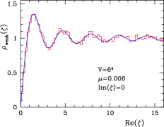
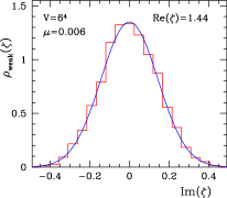
Figure 1: Density of small Dirac eigenvalues for $V=6^{4}$ and $\mu=0.006$, cut along the real axis (left) and parallel to the imaginary axis at the first maximum (right). The histogram represents lattice data, and the solid curve is Eq. (QCD Dirac operator at nonzero chemical potential: lattice data and matrix model).

There is no free fit parameter; the data have been rescaled according to $\xi=\pi\lambda/d$, with $d\propto 1/V$ given in Table 1 (note that $d$ depends on the lattice spacing, i.e. it would change with $\beta$). At weak non-Hermiticity $d$ can be obtained in the same way as for real eigenvalues: Because of the smallness of their imaginary part the eigenvalues can still be ordered with respect to their real part so that the level spacing is defined unambiguously. The very same level spacing $d$ is used to determine $\alpha^{2}=(\pi/\sqrt{2})\,\mu^{2}/d$ from Eq. (7) and $d_{\rm model}=\pi/(\sqrt{2}N)$, leading to $\alpha=0.20$ for use in Eq. (QCD Dirac operator at nonzero chemical potential: lattice data and matrix model). Within our statistical accuracy, we obtain excellent agreement of lattice data and analytical prediction without any free fit parameter.

    

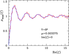
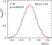
Figure 2: Same as Fig. 1 but for $V=8^{4}$ and $\mu=0.003375$.

In Fig. 2 we repeat the same analysis for lattice size $8^{4}$ and $\mu=0.003375$, chosen to keep $V\mu^{2}=\alpha^{2}$ constant in order to test the scaling predicted by Eq. (7). Here we have used the same value of $\alpha=0.20$ and again find excellent agreement. This value agrees within $0.3\%$ with the value of $\alpha$ determined independently by rescaling $\mu^{2}$ with the level spacing $d$ from the $8^{4}$ data. Similar results are obtained from the analysis of the $10^{4}$ data which we do not display here because of limited statistics.

Next we turn to the limit of strong non-Hermiticity. Here, the eigenvalues are no longer localized close to the real axis and spread into a two-dimensional domain in the complex plane. Therefore we have to modify the determination of the mean level spacing $d$. Nearest neighbors are now defined as having the smallest geometric distance between them. As can be seen from Table 1, the level spacing $d\propto 1/\sqrt{V}$ is very different from the weak limit. The signature of the chiral ensemble (QCD Dirac operator at nonzero chemical potential: lattice data and matrix model) compared to the Ginibre ensemble Gini65 is a “hole” at the origin resulting from the level repulsion. (The latter ensemble applies only in the bulk of the spectrum MPW99 .) To compare the lattice data with Eq. (9), we rescale the eigenvalues according to $\xi=c\lambda/d$, where $c$ is a constant related to the level spacing of our model in the strong non-Hermiticity limit. We currently do not have a theoretical result for $c$ and therefore determined $c=0.82(5)$ by a fit to the data footnote .

    

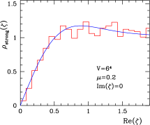
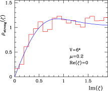
Figure 3: Density of small Dirac eigenvalues for $V=6^{4}$ and $\mu=0.2$, cut along the real (left) and imaginary (right) axes. The histogram represents lattice data, and the solid curve is the prediction of Eq. (9).

    

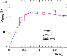
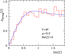
Figure 4: Same as Fig. 3 but for $V=8^{4}$ and $\mu=0.2$.

In Figs. 3 and 4 we plot the data for $\mu=0.2$ and $V=6^{4}$, $8^{4}$ versus the prediction of Eq. (9). Good agreement is found along both the real and imaginary axis (also for $V=10^{4}$, not shown), confirming the rotational invariance of the microscopic density. Note, however, that there is an important difference between the cuts in the real and imaginary directions. While the microscopic density, Eq. (9), is rotationally invariant, the data spread macroscopically into a thin ellipse. Along the imaginary axis the spectrum ends at $\approx\pm 3.8$ in our units, while along the real axis it extends up to $\approx\pm 270$. For that reason the last part of the histograms along the imaginary axis in Figs. 3 and 4 may no longer be in the microscopic regime. In the data for $V=6^{4}$ at intermediate $\mu=0.03$, the microscopic and macroscopic scales no longer separate clearly, and therefore neither of the Eqs. (QCD Dirac operator at nonzero chemical potential: lattice data and matrix model) and (9) apply.

In conclusion, we have identified two different regimes in the behavior of complex eigenvalues of the QCD Dirac operator in the domain where chiral symmetry is broken. Our lattice data confirm the predictions of random matrix theory quantitatively, both at weak and at strong non-Hermiticity. Matrix models thus provide a detailed theoretical understanding of the properties of complex Dirac eigenvalues in a new regime with non-vanishing chemical potential, including the correct scaling of eigenvalues and chemical potential with the volume. Our findings may have algorithmical implications, since it is typically the low-lying Dirac eigenvalues which determine the numerical effort in lattice simulations. We wish to emphasize that, although our conclusions are based on quenched simulations using staggered fermions, the predictions of the matrix model could also be tested in unquenched simulations and in sectors of nontrivial topological charge. This will be the subject of future work.

This work was supported by the DFG (G.A.) and in part by DOE grant No. DE-FG02-91ER40608 (T.W.).

Note added in proof.—The microscopic density of the model Eq. (5) was recently computed in the weak non-Hermiticity limit SV03 . The result deviates very slightly from our Eq. (QCD Dirac operator at nonzero chemical potential: lattice data and matrix model), but this difference cannot be resolved by our data.

In Figs. 1 and 2 we compared lattice data to the analytical prediction of Eq. (5), which pertains to the weak non-Hermiticity limit of the model in Eq. (1). For such a comparison, two independent parameters must be determined: the mean level spacing $d$ and the dimensionless parameter $\alpha$ appearing in Eq. (5). These two parameters can be expressed in terms of two low-energy constants, the chiral condensate $\Sigma$ at $\mu=0$ and the pion decay constant $F_{\pi}$, by the relations $d=\pi/\Sigma V$ and $\alpha^{2}=2\mu^{2}F_{\pi}^{2}V$ AOSV . Here, $V$ is the physical volume. We erroneously determined $\alpha^{2}$ as $(\mu a)^{2}\pi/\sqrt{2}da$, where $a$ is the lattice spacing. This amounts to setting $(F_{\pi}a)^{2}/\Sigma a^{3}=2^{-3/2}$. Instead, $F_{\pi}$ and thus $\alpha$ should be obtained either by an independent measurement of $F_{\pi}$ or by a fit of the data to Eq. (5). Performing the latter for the data sets in Figs. 1 and 2 yields a value of $\alpha=0.200(2)$, which is consistent with the value of $\alpha=0.20$ used in the Letter. Thus, Figs. 1 and 2 as well as the conclusions of the Letter remain unchanged.

The fitting of $\alpha$ to the lattice data constitutes a new method for obtaining $F_{\pi}$ through the relation quoted above, see also Ref. OW , but we refrain from applying this method here since the lattice data were obtained in the strong-coupling region. A related method to determine $F_{\pi}$ using isospin chemical potential was introduced recently in Ref. DHSS .

We thank J.C. Osborn for pointing out the error described above and P.H. Damgaard for useful discussions.

References

- (1) J.J.M. Verbaarschot, H.A. Weidenmüller, and M.R. Zirnbauer, Phys. Rep. 129 (1985) 367
- (2) R. Grobe, F. Haake, and H.-J. Sommers, Phys. Rev. Lett. 61 (1988) 1899
- (3) N. Lehmann and H.-J. Sommers, Phys. Rev. Lett. 67 (1991) 941
- (4) N. Hatano and D.R. Nelson, Phys. Rev. Lett. 77 (1996) 570, J. Miller and J. Wang, Phys. Rev. Lett. 76 (1996) 1461
- (5) M.A. Stephanov, Phys. Rev. Lett. 76 (1996) 4472
- (6) e.g., M. Alford, K. Rajagopal, and F. Wilczek, Nucl. Phys. B 537 (1999) 443 and references therein
- (7) M.A. Halasz et al., Phys. Rev. D 58 (1998) 096007
- (8) Z. Fodor and S.D. Katz, Phys. Lett. B 534 (2002) 87
- (9) C.R. Allton et al., Phys. Rev. D 66 (2002) 074507
- (10) P. de Forcrand and O. Philipsen, Nucl. Phys. B 642 (2002) 290, M. D’Elia and M.-P. Lombardo, Phys. Rev. D67 (2003) 014505
- (11) J. Ambjørn et al., JHEP 0210 (2002) 062
- (12) J.J.M. Verbaarschot and T. Wettig, Ann. Rev. Nucl. Part. Sci. 50 (2000) 343
- (13) G. Akemann, Phys. Rev. Lett. 89 (2002) 072002, J. Phys. A 36 (2003) 3363
- (14) E.V. Shuryak and J.J.M. Verbaarschot, Nucl. Phys. A 560 (1993) 306; J.J.M. Verbaarschot, Phys. Rev. Lett. 72 (1994) 2531
- (15) J. Ginibre, J. Math. Phys. 6 (1965) 440
- (16) G. Akemann, Acta Phys. Polon. B34 (2003) 4653
- (17) Y.V. Fyodorov, B.A. Khoruzhenko, and H.-J. Sommers, Phys. Lett. A 226 (1997) 46, Phys. Rev. Lett. 79 (1997) 557
- (18) P. Hasenfratz and F. Karsch, Phys. Lett. B 125 (1983) 308
- (19) M.E. Berbenni-Bitsch, S. Meyer, and T. Wettig, Phys. Rev. D 58 (1998) 071502; G. Akemann and E. Kanzieper, Phys. Rev. Lett. 85 (2000) 1174; P.H. Damgaard et al., Phys. Lett. B 495 (2000) 263
- (20) J. Smit and J.C. Vink, Nucl. Phys. B 286 (1987) 485
- (21) F. Farchioni, I. Hip, and C.B. Lang, Phys. Lett. B 471 (1999) 58
- (22) R.G. Edwards et al., Phys. Rev. Lett. 82 (1999) 4188
- (23) www.netlib.org/lapack
- (24) www.netlib.org/arpack
- (25) www.cise.ufl.edu/research/sparse/umfpack
- (26) H. Markum, R. Pullirsch, and T. Wettig, Phys. Rev. Lett. 83 (1999) 484
- (27) We have checked for several combinations of and that we obtain the same value for .
- (28) K. Splittorff and J.J.M. Verbaarschot, hep-th/0310271
Erratum: QCD Dirac Operator at Nonzero Chemical Potential:
Lattice Data and Matrix Model
[Phys. Rev. Lett. 92, 102002 (2004)]
Gernot Akemann and Tilo Wettig
(Received 8 December 2005; published 18 January 2006)
PACS numbers: 12.38.Gc, 02.10.Yn, 99.10.Cd

References

- (1) G. Akemann, J.C. Osborn, K. Splittorff, and J.J.M. Verbaarschot, Nucl. Phys. B 712 (2005) 287
- (2) J.C. Osborn and T. Wettig, LATTICE 2005: XXIII International Symposium on Lattice Field Theory [PoS (LAT2005) 200]
- (3) P.H. Damgaard, U.M. Heller, K. Splittorff, and B. Svetitsky, Phys. Rev. D 72 (2005) 091501