KANAZAWA-03-16     
ITEP-LAT-2003-11     
An Abelian effective action reproducing screening and confinement
in quenched SU(2) QCD

Abstract

In an Abelian projection $SU(2)$ gluodynamics contains Abelian gauge fields (diagonal degrees of freedom) and the Abelian matter fields (off-diagonal degrees). The matter fields are essential for the breaking of the adjoint string. We obtain numerically the effective action of Abelian fields in quenched $SU(2)$ QCD and show that the Abelian matter fields provide an essential contribution to the total action even in the infrared region.

The dual superconductor hypothesis [1] was invented to describe the confinement of color in QCD. The model was shown to be quite successful in explanation of the confinement of the fundamental charges such as quarks (see, $e.g.$, reviews [2]). For example, Abelian and monopole contributions to the inter–quark potential are dominant in the long-range region of quenched QCD [3, 4]. The monopole condensation in the confinement phase was also observed [5].

Although the ’t Hooft scenario describes the confinement of the quarks correctly, this scenario predicts also the existence of the string tension for the adjoint charges (gluons) in the infrared region. On the other hand the gluon charges must be screened at large distances due to the presence of the gluons in the QCD vacuum. This screening–confinement problem was discussed within dual superconductor [6] and center vortex formalisms [7].

The standard model of the dual superconductor in the quenched QCD ignores the existence of the off-diagonal gluons. However, these gluons have a charge two with respect to the Abelian subgroup and they may explain the flattening of the inter–gluon potential which is usually studied with the help of the adjoint Wilson loop. On the other hand the introduction of the new degrees of freedom – the off-diagonal gluons – should not violate already achieved success of the explanation of the quark confinement in this model. Indeed, quarks have the charge one and doubly charged gluons can not screen them.

To reproduce the screening of charge two we must keep all doubly charged Abelian Wilson loops in the effective action of the Abelian link fields. The theory in terms of the Abelian link fields or the Abelian monopole currents alone becomes highly non–local if we integrate out all off-diagonal gluon fields after an Abelian projection.

Needless to say, such an Abelian effective action is useless. The same problem is more serious in the real full QCD, since the fundamental charge is also screened in this case.

We calculate numerically the effective action of quenched QCD within the Abelian projection formalism. Contrary to previous calculations of this kind we include also the doubly charged off-diagonal gluon fields into the effective action and we show that their contribution is essential in the infrared region and thus can not be neglected.

The Wilson action of the quenched $SU(2)$ QCD is $S=\beta/2\sum_{s,\mu,\nu}\,{\mathrm{Tr}}\,U_{\mu\nu}(s)$, where $U_{\mu\nu}$ is the standard $SU(2)$ plaquette. We parameterize the $SU(2)$ link as $U_{\mu}(s)=c_{\mu}(s)u_{\mu}(s)$, where $u_{\mu}(s)={\mathrm{diag}}(e^{i\theta_{\mu}(s)},e^{-i\theta_{\mu}(s)})$ and

$$c_{\mu}(s)=\left(\begin{array}[]{@{}cc@{}}\cos\phi_{\mu}(s)&i\sin\phi_{\mu}(s)e^{-i\varphi_{\mu}(s)}\\ i\sin\phi_{\mu}(s)e^{i\varphi_{\mu}(s)}&\cos\phi_{\mu}(s)\end{array}\right).$$ (3)

The independent variables, $\theta$, $\varphi$, $\phi$, are restricted: $-\pi\leq\theta_{\mu}(s),\varphi_{\mu}(s)<\pi$, $0\leq\phi_{\mu}(s)<\pi/2$.

Under the Abelian gauge transformation, $\Omega^{\mathrm{Abel}}(\omega)={\mathrm{diag}(e^{i\alpha(s)},e^{-i\alpha(s)})}$, the field $\theta$ behaves as the $U(1)$ gauge field, $\theta_{\mu}(s)\to\theta_{\mu}(s)+\alpha(s)-\alpha(s+\hat{\mu})$, while the field $\varphi$ corresponds to a phase of the off–diagonal gluon field, $\varphi_{\mu}(s)\to\varphi_{\mu}(s)+2\alpha(s)$. The variable $\phi_{\mu}(s)$ is not affected by the $U(1)$ gauge transformation.

If an Abelian gauge is fixed we can integrate the $\phi_{\mu}(s)$ variable out without harming the $U(1)$ content of the model. In order to get possible forms of interactions between the Abelian gauge and Abelian matter fields let us replace the averages of $\cos\phi_{\mu}(s)$ and $\sin\phi_{\mu}(s)$ by their mean values in the Maximal Abelian gauge [8, 9]:

$$\begin{array}[]{rcl}\cos\phi_{\mu}(s)&\to&\langle\cos\phi_{\mu}(s)\rangle\equiv c\simeq 1\,,\\ \sin\phi_{\mu}(s)&\to&\langle\sin\phi_{\mu}(s)\rangle\equiv s\ll c\,,\end{array}$$ (6)

Then we get an action of the SU(2) model as

$$\begin{array}[]{rcl}\Theta_{\mu\nu}(s)\!\!\!\!&=&\!\!\!\!\theta_{\mu}(s)+\theta_{\nu}(s+\hat{\mu})-\theta_{\mu}(s+\hat{\nu})-\theta_{\nu}(s),\\ H_{\mu\nu}(s)\!\!\!\!&=&\!\!\!\!2\theta_{\mu}(s)+\varphi_{\nu}(s)-\varphi_{\nu}(s+\hat{\mu})\,,\\ C_{\mu\nu}(s)\!\!\!\!&=&\!\!\!\!\varphi_{\mu}(s)-\varphi_{\nu}(s)\,,\end{array}$$ (10)

where $\Theta$ is the $U(1)$ plaquette for the gauge field, $H$ describes the interaction of the matter and gauge fields, and $C$ corresponds to the self–interaction of the matter field. Similarly to Ref. [9] we get:

$$\frac{1}{2}{\mathrm{Tr}}\,U_{\mu\nu}(s)=c^{4}\cos(\Theta_{\mu\nu}(s))$$

$$+c^{2}s^{2}\cos(\Theta_{\mu\nu}(s)+C_{\mu\nu}(s))$$

$$+[-c^{2}s^{2}\cos(\Theta_{\mu\nu}(s)-H_{\mu\nu}(s)-C_{\mu\nu}(s))$$

$$+c^{2}s^{2}\cos(\Theta_{\mu\nu}(s)-H_{\mu\nu}(s))+(\mu\leftrightarrow\nu)]$$

$$+c^{2}s^{2}\cos(\Theta_{\mu\nu}(s)-H_{\mu\nu}(s)+H_{\nu\mu}(s)-C_{\mu\nu}(s))$$

$$+s^{4}\cos(\Theta_{\mu\nu}(s)-H_{\mu\nu}(s)+H_{\nu\mu}(s)-2C_{\mu\nu}(s)).$$

Hence we chose, for our numerical study, a trial action

$$S_{\mathrm{eff}}(\theta,\varphi)=\sum\nolimits_{i=1}^{3}\alpha_{i}S_{i}(\theta)+\beta_{1}S_{4}(\theta,\varphi)\,,$$ (11)

where $\alpha_{i}$, $i=1,2,3$ and $\beta_{1}$ are the couplings and

$$S_{k}=-\sum\nolimits_{s,\mu\neq\nu}\cos k\Theta_{\mu\nu}(s)\,,\quad k=1,2\,,$$

$$S_{3}=+\sum\nolimits_{s,\mu\neq\nu}\sin\Theta_{\mu\nu}(s)\sin\Theta_{\mu\nu}(s+\hat{\mu})\,,$$ (12)

$$S_{4}=-\sum_{s,\mu\neq\nu}\Bigl{[}\cos(\Theta_{\mu\nu}(s)-H_{\mu\nu}(s))+(\mu\leftrightarrow\nu)\Bigr{]}\,.$$

The action $S_{1}$ is the leading term in the Abelian action in the mean–field approximation (6). The terms $S_{2,3}$ may arise from the integration over $\phi$ fields. The action $S_{4}$ describes interaction of the gauge, $\theta$, and the matter, $\varphi$, fields.

We have used the standard Monte–Carlo procedure to generate the gauge field configurations on the $32^{4}$ lattice at $\beta=2.1\sim 2.7$. We have generated 100 configurations of the gauge field for each value of the coupling constant and then used the Simulated Annealing method [4] to fix the Maximal Abelian gauge. The couplings $\alpha_{i}$, $i=1,2,3$ and $\beta_{1}$ were determined by solving the Schwinger–Dyson equations [10]. We further improve our results towards the continuum limit using a blockspin transformation for the $SU(2)$ link variable $U_{\mu}$ visualized in Figure 1.

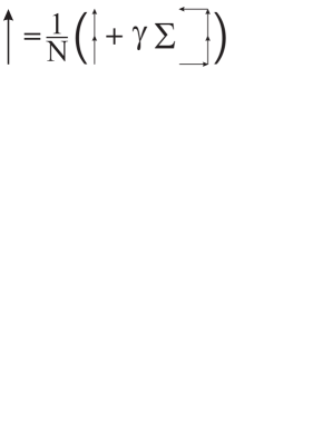
Figure 1: The blockspin transformation. The normalization factor, $N\equiv N(U)$, is introduced to make the fat link belonging to the $SU(2)$ group. The weight parameter $\gamma$ is set to $1/2$.

In Figure 2 we show the couplings of the action (11) $vs.$ the scale $b=na$ where $n$ corresponds to the blockspin factor and $a$ is the lattice spacing. The scale $b$ is shown in units of the string tension. The coupling $\alpha_{1}$ shows a perfect scaling for all $n$ while the other couplings scale for $n>1$ only. Thus at small values of $b$ the effective action is more complicated than (11). A similar effect is found for the monopole action [11].

We have fitted the data for couplings by

$$f(b)=C_{0}+C_{1}\exp\{-({b/b_{0})}^{\nu}\}\,,$$ (13)

where $C_{0,1}$, $\nu$ and $b_{0}$ are the fitting parameters. In our fits the data with $n=1$ is excluded for all coupling constants except for $\alpha_{1}$. The best fit curves are plotted in Figures 2, and the best fit parameters are shown in Table 1.

In the case of $\alpha_{1}$ and $\beta_{1}$ the parameter $\nu$ is very close to two, therefore we fixed this parameter, $\nu=2$. Similarly, we have set $\nu=1$ for $\alpha_{2}$ and $C_{0}=0$ for $\alpha_{2,3}$. Note that the fit can not describe accurately the couplings $\alpha_{1}$ and $\alpha_{3}$ at small scales, $b\leqslant 0.2$ fm, where the Abelian action is expected to be more complicated than (11).

Figure 2: The parameters $\alpha_{i}$ and $\beta_{1}$ $vs.$ $b$. The fits by Eq. (13) are shown by the dashed lines.

The functional $S_{1}$ makes the leading contribution to the action since the coupling $\alpha_{1}$ is the largest one. The actions $S_{2}$ and $S_{3}$ play an essential role only at small distances. The action $S_{4}$, which describes the interaction of the matter fields with the gauge fields is non–vanishing at large scales similarly to $S_{1}$. Moreover, the couplings $\alpha_{1}$ and $\beta_{1}$ have larger lengths $b_{0}$ compared to $\alpha_{2}$ and $\alpha_{3}$.

	$C_{0}$	$C_{1}$	$b_{0}$, [fm]	$\nu$
$\alpha_{1}$	0.066(10)	1.20(2)	0.61(1)	2
$\alpha_{2}$	0	0.32(2)	0.231(7)	1
$\alpha_{3}$	0	-0.28(3)	0.46(3)	1.8(2)
$\beta_{1}$	0.064(5)	0.30(1)	0.69(2)	2

Table 1:

Thus, at large scales, $b\sqrt{\sigma}\gg 1$, the effective Abelian action for the $SU(2)$ gauge theory can be approximated as a sum of the QED–like action for the gauge field, $S_{1}(\theta)$, and the interaction term $S_{4}(\theta,\varphi)$. This is the manifestation of the Abelian dominance (non–vanishing dominant coupling $\alpha_{1}$) and the importance of the off-diagonal (matter) degrees of freedom (non–vanishing coupling $\beta_{1}$). The matter fields are essential for the breaking of the adjoint string.

References

- [1] G. ’t Hooft, in High Energy Physics, ed. A. Zichichi, EPS International Conference, Palermo (1975); S. Mandelstam, Phys. Rept. 23 (1976) 245.
- [2] T. Suzuki, Nucl. Phys. Proc. Suppl. 30 (1993) 176; M. N. Chernodub, M. I. Polikarpov, in ”Confinement, duality, and nonperturbative aspects of QCD”, Ed. by P. van Baal, Plenum Press, p. 387, hep-th/9710205; R.W. Haymaker, Phys. Rept. 315 (1999) 153.
- [3] T. Suzuki, I. Yotsuyanagi, Phys. Rev. D42 (1990) 4257; H. Shiba, T. Suzuki, Phys. Lett. B 333 (1994) 461; T. Suzuki, in Continuous Advances in QCD 1996 (World Scientific, 1997), p. 262; J. D. Stack, S. D. Neiman and R. J. Wensley, Phys. Rev. D 50 (1994) 3399.
- [4] G. S. Bali et al, Phys. Rev. D 54 (1996) 2863.
- [5] N. Arasaki et al, Phys. Lett. B 395 (1997) 275; K. Yamagishi, T. Suzuki, S. i. Kitahara, JHEP 0002 (2000) 012; M. N. Chernodub, M. I. Polikarpov, A. I. Veselov, Phys. Lett. B 399, 267 (1997); Nucl. Phys. Proc. Suppl. 49 (1996) 307; A. Di Giacomo, G. Paffuti, Phys. Rev. D 56 (1997) 6816; H. Shiba, T. Suzuki, Phys. Lett. B351 (1995) 519.
- [6] T. Suzuki and M. N. Chernodub, Phys. Lett. B 563 (2003) 183.
- [7] L. Del Debbio et al, Phys. Rev. D 58 (1998) 094501; J. Ambjørn et al, JHEP 0002 (2000) 033.
- [8] T. Suzuki and I. Yotsuyanagi, Nucl. Phys. Proc. Suppl. 20 (1991) 236.
- [9] M. N. Chernodub, M. I. Polikarpov and A. I. Veselov, Phys. Lett. B 342 (1995) 303.
- [10] A. Gonzalez-Arroyo, M. Okawa, Phys. Rev. D 35 (1987) 672; Phys. Rev. B 35 (1987) 2108.
- [11] M. N. Chernodub, et al, Phys. Rev. D 62, 094506 (2000); hep-lat/9902013.