Electromagnetic Properties of the Baryon Decuplet in
Quenched and Partially Quenched Chiral Perturbation Theory

Abstract

We calculate electromagnetic properties of the decuplet baryons in quenched and partially quenched chiral perturbation theory. We work at next-to-leading order in the chiral expansion, leading order in the heavy baryon expansion, and obtain expressions for the magnetic moments, charge radii, and electric quadrupole moments. The quenched calculation is shown to be pathological since only quenched chiral singularities are present at this order. We present the partially quenched results for both the $SU(2)$ and $SU(3)$ flavor groups and use the isospin limit in the latter. These results are necessary for proper extrapolation of lattice calculations of decuplet electromagnetic properties.

I Introduction

The study of hadronic electromagnetic properties provides important insight into the non-perturbative structure of QCD. A model-independent tool to study QCD at low energies is chiral perturbation theory ($\chi$PT), which is an effective field theory with low-energy degrees of freedom, e.g., the meson octet in $SU(3)$ flavor. $\chi$PT assumes that these mesons are the pseudo-Goldstone bosons that appear from spontaneous breaking of chiral symmetry from $SU(3)_{L}\otimes SU(3)_{R}$ down to $SU(3)_{V}$. Observables receive contributions from both long-range and short range physics; in $\chi$PT the long-range contribution arises from the (non-analytic) pion loops, while the short-range contribution arises from low-energy constants. The number of these low-energy constants is constrained by symmetries but their values must be determined from experiment or lattice simulations.

Progress in measuring the proton and neutron form factors has been made (see Mergell et al. (1996); Hammer et al. (1996) for references), including recent high precision measurements for the proton Gayou et al. (2002). Experimental study of the remaining baryons, in particular the decuplet baryon resonances, however, is much harder. Experiments measuring the decuplet magnetic moments are anticipated in the foreseeable future. The Particle Data Group lists values for the ${\Delta}^{++}$ magnetic moment Hagiwara et al. (2002) but with sizeable discrepancy and uncertainty, even among the two most recent results Bosshard et al. (1991); Lopez Castro and Mariano (2002). A report of the initial measurement of the ${\Delta}^{+}$ magnetic moment Kotulla et al. (2002) has recently appeared, and further data are eagerly awaited.

Although more experimental data for the other decuplet electromagnetic moments can be expected in the future, progress will be slow due to significant experimental difficulties. Theory, however, may be able to catch up. While lattice calculations using the quenched approximation have already appeared Leinweber et al. (1992), we expect partially quenched calculations for decuplet observables in the near future. One problem that currently and foreseeably plagues these lattice calculations is that they are performed with unphysically large quark masses. Therefore, to make physical predictions, one must extrapolate from the heavier quark masses used on the lattice (currently on the order of the strange quark mass) down to the physical light quark masses. For quenched QCD (QQCD) lattice calculations, where the fermion determinant that arises from the path integral is set equal to one, one uses quenched chiral perturbation theory (Q$\chi$PT) Morel (1987); Sharpe (1992); Bernard and Golterman (1992a, b); Golterman (1994); Sharpe and Zhang (1996); Labrenz and Sharpe (1996) to extrapolate. The problem with the quenched approximation is that the Goldstone boson singlet, the $\eta^{\prime}$, which is heavy in QCD, remains light and must be included in the Q$\chi$PT Lagrangian. This requires new operators and hence new low-energy constants. Thus in general, the low-energy constants appearing in Q$\chi$PT are unrelated to those in $\chi$PT and extrapolated quenched lattice data is unrelated to QCD. In fact, several examples show that the behavior of meson loops near the chiral limit is frequently misrepresented in Q$\chi$PT Booth (1994); Kim and Kim (1998); Savage (2002a); Arndt (2003); Dong et al. (2003); Arndt and Tiburzi (2003). We find this to be true for the decuplet electromagnetic observables. Indeed, to the order we work only quenched chiral singularities are present in the quenched electromagnetic moments; the charge radii have no quark mass dependence at all.

The unattractive features of QQCD can be remedied by using partially quenched lattice QCD (PQQCD). Unlike in QQCD, where the “sea quarks” are neglected by setting the fermion determinant to unity, in PQQCD these sea quarks are kept as dynamical degrees of freedom and their masses can be varied independently of the valence quark masses. For computational reasons they are usually chosen to be heavier. The low-energy effective theory of PQQCD is PQ$\chi$PT Bernard and Golterman (1994); Sharpe (1997); Golterman and Leung (1998); Sharpe and Shoresh (2000a, 2001a, b, 2001b); Shoresh (2001). Since PQQCD retains a $U(1)_{A}$ anomaly, the equivalent to the singlet field in QCD is heavy (on the order of the chiral symmetry breaking scale ${\Lambda}_{\chi}$) and can be integrated out Sharpe and Shoresh (2001a, b). Therefore, the low-energy constants appearing in PQ$\chi$PT are the same as those appearing in $\chi$PT. By fitting PQ$\chi$PT to partially quenched lattice data one can determine these constants and actually make physical predictions for QCD. PQ$\chi$PT has been used recently to study heavy meson Savage (2002b) and octet baryon observables Chen and Savage (2002); Beane and Savage (2002a); Savage (2002c); Leinweber (2002); Arndt and Tiburzi (2003).

While there has been a quenched lattice calculation of the decuplet magnetic moments Leinweber et al. (1992), there are currently no partially quenched simulations. However, in light of the progress that lattice gauge theory has made recently in the one-hadron sector and the prospect of simulations in the two-hadron sector LAT (a, b); Beane and Savage (2003, 2002b); Arndt et al. (2003), we expect to see partially quenched calculations of the decuplet electromagnetic form factors in the near future.

The paper is organized as follows. First, in Section II, we review PQ$\chi$PT including the treatment of the baryon octet and decuplet in the heavy baryon approximation. In Section III, we calculate the electromagnetic moments and charge radii of the decuplet baryons in both Q$\chi$PT and PQ$\chi$PT up to next-to-leading (NLO) order in the chiral expansion. We use the heavy baryon formalism of Jenkins and Manohar Jenkins and Manohar (1991a, b), and work to lowest order in the heavy baryon expansion. These calculations are done in the isospin limit of $SU(3)$ flavor. Expressions for form factors with the $q^{2}$ dependence at one loop are given in Appendix A. For completeness we also provide the PQ$\chi$PT result for the baryon quartet electromagnetic moments and charge radii for the $SU(2)$ chiral Lagrangian with non-degenerate quarks in Appendix B. We conclude in Section IV.

II PQ$\chi$PT

In PQQCD the quark part of the Lagrangian is written as Sharpe and Shoresh (2001a, b, 2000b, 2000a); Golterman and Leung (1998); Sharpe (1997); Bernard and Golterman (1994); Shoresh (2001)

$${\cal L} = \sum_{a,b=u,d,s}\bar{q}_{a}(iD\hskip-6.49994pt/-m_{q})_{ab}q_{b}+\sum_{\tilde{a},\tilde{b}=\tilde{u},\tilde{d},\tilde{s}}\bar{\tilde{q}}_{\tilde{a}}(iD\hskip-6.49994pt/-m_{\tilde{q}})_{\tilde{a}\tilde{b}}\tilde{q}_{\tilde{b}}+\sum_{a,b=j,l,r}\bar{q}_{\text{sea},a}(iD\hskip-6.49994pt/-m_{\text{sea}})_{ab}q_{\text{sea},b}$$ (1)

$$=\sum_{j,k=u,d,s,\tilde{u},\tilde{d},\tilde{s},j,l,r}\bar{Q}_{j}(iD\hskip-6.49994pt/-m_{Q})_{jk}Q_{k}.$$

Here, in addition to the fermionic light valence quarks $u$, $d$, and $s$, their bosonic counterparts $\tilde{u}$, $\tilde{d}$, and $\tilde{s}$ (the ghost quarks) and three light fermionic sea quarks $j$, $l$, and $r$ have been added. These nine quarks are in the fundamental representation of the graded group $SU(6|3)$ Balantekin et al. (1981); Balantekin and Bars (1981, 1982) and appear in the vector

$$Q=(u,d,s,j,l,r,\tilde{u},\tilde{d},\tilde{s})$$ (2)

that obeys the graded equal-time commutation relation

$$Q^{\alpha}_{i}({\bf x}){Q^{\beta}_{j}}^{\dagger}({\bf y})-(-1)^{\eta_{i}\eta_{j}}{Q^{\beta}_{j}}^{\dagger}({\bf y})Q^{\alpha}_{i}({\bf x})={\delta}^{{\alpha}{\beta}}{\delta}_{ij}{\delta}^{3}({\bf x}-{\bf y}),$$ (3)

where ${\alpha}$ and ${\beta}$ are spin and $i$ and $j$ are flavor indices. The graded equal-time commutation relations for two $Q$’s and two $Q^{\dagger}$’s can be written analogously. The grading factor

$$\eta_{k}=\left\{\begin{array}[]{cl}1&\text{for }k=1,2,3,4,5,6\\ 0&\text{for }k=7,8,9\end{array}\right.$$ (4)

reflects the different statistics for fermionic and bosonic quarks. The quark mass matrix is given by

$$m_{Q}=\text{diag}(m_{u},m_{d},m_{s},m_{j},m_{l},m_{r},m_{u},m_{d},m_{s})$$ (5)

so that diagrams with closed ghost quark loops cancel those with valence quarks. Effects of virtual quark loops are, however, present due to the finite-mass sea quarks. In the limit $m_{j}=m_{u}$, $m_{l}=m_{d}$, and $m_{r}=m_{s}$ one recovers QCD.

The light quark electric charge matrix ${\mathcal{Q}}$ is not uniquely defined in PQQCD Golterman and Pallante (2002). The only constraint one imposes is for the charge matrix ${\mathcal{Q}}$ to have vanishing supertrace, so that no new operators involving the singlet component are subsequently introduced. Following the convention in Chen and Savage (2002), we use

$${\mathcal{Q}}=\text{diag}\left(\frac{2}{3},-\frac{1}{3},-\frac{1}{3},q_{j},q_{l},q_{r},q_{j},q_{l},q_{r}\right).$$ (6)

When $m_{j}\to m_{u}$, $m_{l}\to m_{d}$, and $m_{r}\to m_{s}$, QCD is recovered independently of the $q$’s.

II.1 Mesons

For massless quarks, the Lagrangian in Eq. (1) exhibits a graded symmetry $SU(6|3)_{L}\otimes SU(6|3)_{R}\otimes U(1)_{V}$ that is assumed to be spontaneously broken down to $SU(6|3)_{V}\otimes U(1)_{V}$. The low-energy effective theory of PQQCD that emerges by expanding about the physical vacuum state is PQ$\chi$PT. The dynamics of the emerging 80 pseudo-Goldstone mesons can be described at lowest order in the chiral expansion by the Lagrangian

$${\cal L}=\frac{f^{2}}{8}\text{str}\left(D^{\mu}\Sigma^{\dagger}D_{\mu}\Sigma\right)+{\lambda}\,\text{str}\left(m_{Q}\Sigma+m_{Q}^{\dagger}\Sigma^{\dagger}\right)+{\alpha}\partial^{\mu}\Phi_{0}\partial_{\mu}\Phi_{0}-\mu_{0}^{2}\Phi_{0}^{2}$$ (7)

where

$$\Sigma=\exp\left(\frac{2i\Phi}{f}\right)=\xi^{2},$$ (8)

$$\Phi=\left(\begin{array}[]{cc}M&\chi^{\dagger}\\ \chi&\tilde{M}\end{array}\right),$$ (9)

$f=132$ MeV, and the gauge-covariant derivative is $D_{\mu}{\Sigma}=\partial_{\mu}{\Sigma}+ie{\mathcal{A}}_{\mu}[{\mathcal{Q}},{\Sigma}]$. The str() denotes a supertrace over flavor indices. The $M$, $\tilde{M}$, and $\chi$ are matrices of pseudo-Goldstone bosons with quantum numbers of $q{\overline{q}}$ pairs, pseudo-Goldstone bosons with quantum numbers of $\tilde{q}{\overline{\tilde{q}}}$ pairs, and pseudo-Goldstone fermions with quantum numbers of $\tilde{q}{\overline{q}}$ pairs, respectively. $\Phi$ is defined in the quark basis and normalized such that $\Phi_{12}=\pi^{+}$ (see, for example, Chen and Savage (2002)). Upon expanding the Lagrangian in (7) one finds that to lowest order the mesons with quark content $Q\bar{Q^{\prime}}$ are canonically normalized when their masses are given by

$$m_{QQ^{\prime}}^{2}=\frac{4\lambda}{f^{2}}(m_{Q}+m_{Q^{\prime}}).$$ (10)

The flavor singlet field given by $\Phi_{0}=\text{str}(\Phi)/\sqrt{6}$ is, in contrast to the Q$\chi$PT case, rendered heavy by the $U(1)_{A}$ anomaly and can therefore be integrated out in $\chi$PT. Analogously its mass $\mu_{0}$ can be taken to be on the order of the chiral symmetry breaking scale, $\mu_{0}\to\Lambda_{\chi}$. In this limit the flavor singlet propagator becomes independent of the coupling ${\alpha}$ and deviates from a simple pole form Sharpe and Shoresh (2001a, b).

II.2 Baryons

Just as there are mesons in PQQCD with quark content ${\overline{Q}}_{i}Q_{j}$ that contain valence, sea, and ghost quarks, there are baryons with quark composition $Q_{i}Q_{j}Q_{k}$ that contain all three types of quarks. Restrictions on the baryon fields ${\mathcal{B}}_{ijk}$ come from the fact that these fields must reproduce the familiar octet and decuplet baryons when $i$, $j$, $k=1$-$3$ Labrenz and Sharpe (1996); Chen and Savage (2002). To this end, one decomposes the irreducible representations of $SU(6|3)_{V}$ into irreducible representations of $SU(3)_{\text{val}}\otimes SU(3)_{\text{sea}}\otimes SU(3)_{\text{ghost}}\otimes U(1)$. The method to construct the octet baryons is to use the interpolating field

$${\mathcal{B}}_{ijk}^{\gamma}\sim\left(Q_{i}^{{\alpha},a}Q_{j}^{{\beta},b}Q_{k}^{{\gamma},c}-Q_{i}^{{\alpha},a}Q_{j}^{{\gamma},c}Q_{k}^{{\beta},b}\right){\epsilon}_{abc}(C{\gamma}_{5})_{{\alpha}{\beta}}.$$ (11)

The spin-1/2 baryon octet $B_{ijk}={\mathcal{B}}_{ijk}$, where the indices $i$, $j$, and $k$ are restricted to $1$–$3$, is contained as a $(\bf 8,\bf 1,\bf 1)$ of $SU(3)_{\text{val}}\otimes SU(3)_{\text{sea}}\otimes SU(3)_{\text{ghost}}$ in the $\bf 240$ representation. The octet baryons, written in the familiar two-index notation

$$B=\left(\begin{array}[]{ccc}\frac{1}{\sqrt{6}}{\Lambda}+\frac{1}{\sqrt{2}}{\Sigma}^{0}&{\Sigma}^{+}&p\\ {\Sigma}^{-}&\frac{1}{\sqrt{6}}{\Lambda}-\frac{1}{\sqrt{2}}{\Sigma}^{0}&n\\ \Xi^{-}&\Xi^{0}&-\frac{2}{\sqrt{6}}{\Lambda}\end{array}\right),$$ (12)

are embedded in $B_{ijk}$ as Labrenz and Sharpe (1996)

$$B_{ijk}=\frac{1}{\sqrt{6}}\left({\epsilon}_{ijl}B_{kl}+{\epsilon}_{ikl}B_{jl}\right).$$ (13)

Besides the conventional octet baryons that contain valence quarks, $qqq$, there are also baryon fields with sea and ghost quarks contained in the $\bf 240$, e.g., $qq_{\text{sea}}\tilde{q}$. The baryon states needed for our calculation have at most one ghost or one sea quark and have been constructed explicitly in Chen and Savage (2002).

Similarly, the familiar spin-3/2 decuplet baryons are embedded in the $\bf 165$. Here, one uses the interpolating field

$${\mathcal{T}}_{ijk}^{{\alpha},\mu}\sim\left(Q_{i}^{{\alpha},a}Q_{j}^{{\beta},b}Q_{k}^{{\gamma},c}+Q_{i}^{{\beta},b}Q_{j}^{{\gamma},c}Q_{k}^{{\alpha},a}+Q_{i}^{{\gamma},c}Q_{j}^{{\alpha},a}Q_{k}^{{\beta},b}\right){\epsilon}_{abc}\left(C{\gamma}^{\mu}\right)_{{\beta}{\gamma}}$$ (14)

that describes the $\bf 165$ dimensional representation of $SU(6|3)_{V}$. The decuplet baryons $T_{ijk}$ are then readily embedded in ${\mathcal{T}}$ by construction: $T_{ijk}={\mathcal{T}}_{ijk}$, where the indices $i$, $j$, and $k$ are restricted to $1$–$3$. They transform as a $(\bf 10,\bf 1,\bf 1)$ under $SU(3)_{\text{val}}\otimes SU(3)_{\text{sea}}\otimes SU(3)_{\text{ghost}}$. Because of Eqs. (3) and (14), $T_{ijk}$ is a totally symmetric tensor. Our normalization convention is such that $T_{111}={\Delta}^{++}$. For the spin-3/2 baryons consisting of two valence and one ghost quark or two valence and one sea quark, we use the states constructed in Chen and Savage (2002).

At leading order in the heavy baryon expansion, the free Lagrangian for the ${\mathcal{B}}_{ijk}$ and ${\mathcal{T}}_{ijk}$ is given by Labrenz and Sharpe (1996)

$${\mathcal{L}} = i\left({\overline{{\mathcal{B}}}}v\cdot{\mathcal{D}}{\mathcal{B}}\right)+2{\alpha}_{M}\left({\overline{{\mathcal{B}}}}{\mathcal{B}}{\mathcal{M}}_{+}\right)+2{\beta}_{M}\left({\overline{{\mathcal{B}}}}{\mathcal{M}}_{+}{\mathcal{B}}\right)+2\sigma_{M}\left({\overline{{\mathcal{B}}}}{\mathcal{B}}\right)\text{str}\left({\mathcal{M}}_{+}\right)$$ (15)

$$-i\left({\overline{{\mathcal{T}}}}^{\mu}v\cdot{\mathcal{D}}{\mathcal{T}}_{\mu}\right)+{\Delta}\left({\overline{{\mathcal{T}}}}^{\mu}{\mathcal{T}}_{\mu}\right)+2{\gamma}_{M}\left({\overline{{\mathcal{T}}}}^{\mu}{\mathcal{M}}_{+}{\mathcal{T}}_{\mu}\right)-2{\overline{\sigma}}_{M}\left({\overline{{\mathcal{T}}}}^{\mu}{\mathcal{T}}_{\mu}\right)\text{str}\left({\mathcal{M}}_{+}\right),$$

where ${\mathcal{M}}_{+}=\frac{1}{2}\left(\xi^{\dagger}m_{Q}\xi^{\dagger}+\xi m_{Q}\xi\right)$. The brackets in (15) are shorthands for field bilinear invariants originally employed in Labrenz and Sharpe (1996). To lowest order in the chiral expansion, Eq. (15) gives the propagators

$$\frac{i}{v\cdot k},\quad\frac{iP^{\mu\nu}}{v\cdot k-{\Delta}}$$ (16)

for the spin-1/2 and spin-3/2 baryons, respectively. Here, $v$ is the velocity and $k$ the residual momentum of the heavy baryon which are related to the momentum $p$ by $p=M_{B}v+k$. $M_{B}$ denotes the (degenerate) mass of the octet baryons and ${\Delta}$ the decuplet–baryon mass splitting. The polarization tensor

$$P^{\mu\nu}=\left(v^{\mu}v^{\nu}-g^{\mu\nu}\right)-\frac{4}{3}S_{v}^{\mu}S_{v}^{\nu}$$ (17)

reflects the fact that the Rarita-Schwinger field $({\mathcal{T}}^{\mu})_{ijk}$ contains both spin-1/2 and spin-3/2 pieces; only the latter remain as propagating degrees of freedom Jenkins and Manohar (1991b).

The Lagrangian describing the relevant interactions of the ${\mathcal{B}}_{ijk}$ and ${\mathcal{T}}_{ijk}$ with the pseudo-Goldstone mesons is

$${\cal L}=2{\mathcal{H}}\left({\overline{{\mathcal{T}}}}^{\nu}S^{\mu}A_{\mu}{\mathcal{T}}_{\nu}\right)+\sqrt{\frac{3}{2}}{\mathcal{C}}\left[\left({\overline{{\mathcal{T}}}}^{\nu}A_{\nu}{\mathcal{B}}\right)+\text{h.c.}\right].$$ (18)

The axial-vector and vector meson fields $A^{\mu}$ and $V^{\mu}$ are defined by analogy to those in QCD:

$$A^{\mu}=\frac{i}{2}\left(\xi\partial^{\mu}\xi^{\dagger}-\xi^{\dagger}\partial^{\mu}\xi\right)\quad\text{and}\quad V^{\mu}=\frac{1}{2}\left(\xi\partial^{\mu}\xi^{\dagger}+\xi^{\dagger}\partial^{\mu}\xi\right).$$ (19)

The latter appears in Eq. (18) in the covariant derivatives of ${\mathcal{B}}_{ijk}$ and ${\mathcal{T}}_{ijk}$ that both have the form

$$({\mathcal{D}}^{\mu}{\mathcal{B}})_{ijk}=\partial^{\mu}{\mathcal{B}}_{ijk}+(V^{\mu})_{il}{\mathcal{B}}_{ljk}+(-)^{\eta_{i}(\eta_{j}+\eta_{m})}(V^{\mu})_{jm}{\mathcal{B}}_{imk}+(-)^{(\eta_{i}+\eta_{j})(\eta_{k}+\eta_{n})}(V^{\mu})_{kn}{\mathcal{B}}_{ijn}.$$ (20)

III Decuplet electromagnetic properties

The electromagnetic moments of decuplet baryons in $\chi$PT have been investigated previously in Butler et al. (1994); Banerjee and Milana (1996). Additionally there has been interest in the decuplet electromagnetic properties in the large $N_{c}$ limit of QCD Buchmann and Lebed (2000); Buchmann et al. (2002); Buchmann and Lebed (2003); Cohen (2003). In this Section we calculate the decuplet electromagnetic moments and charge radii in PQ$\chi$PT and Q$\chi$PT. The basic conventions and notations for the mesons and baryons in PQ$\chi$PT have been laid forth in the last Section; Q$\chi$PT has been extensively reviewed in the literature Morel (1987); Sharpe (1992); Bernard and Golterman (1992a, b); Golterman (1994); Sharpe and Zhang (1996); Labrenz and Sharpe (1996). Additionally the decuplet charge radii in $\chi$PT are provided since they have not been calculated before. First we review the electromagnetic form factors of heavy spin-$3/2$ baryons.

Using the heavy baryon formalism Jenkins and Manohar (1991a, b), the decuplet matrix elements of the electromagnetic current $J^{\rho}$ can be parametrized as

$$\langle{\overline{T}}(p^{\prime})|J^{\rho}|T(p)\rangle=-{\overline{u}}_{\mu}(p^{\prime})\mathcal{O}^{\mu\rho\nu}u_{\nu}(p),$$ (21)

where $u_{\mu}(p)$ is a Rarita-Schwinger spinor for an on-shell heavy baryon satisfying $v^{\mu}u_{\mu}(p)=0$ and $S^{\mu}u_{\mu}(p)=0$. The tensor $\mathcal{O}^{\mu\rho\nu}$ can be parametrized in terms of four independent, Lorentz invariant form factors

$$\mathcal{O}^{\mu\rho\nu}=g^{\mu\nu}\left\{v^{\rho}F_{1}(q^{2})+\frac{[S^{\rho},S^{\tau}]}{M_{B}}q_{\tau}F_{2}(q^{2})\right\}+\frac{q^{\mu}q^{\nu}}{(2M_{B})^{2}}\left\{v^{\rho}G_{1}(q^{2})+\frac{[S^{\rho},S^{\tau}]}{M_{B}}q_{\tau}G_{2}(q^{2})\right\},$$ (22)

where the momentum transfer $q=p^{\prime}-p$. The form factor $F_{1}(q^{2})$ is normalized to the decuplet charge in units of $e$: $F_{1}(0)=Q$. At NLO in the chiral expansion, the form factor $G_{2}(q^{2})=0$.

Extraction of the form factors requires a nontrivial identity for on-shell Rarita-Schwinger spinors Nozawa and Leinweber (1990). For heavy baryon spinors, the identity is

$${\overline{u}}_{\alpha}(p^{\prime})\big{(}q^{\alpha}g^{\mu\beta}-q^{\beta}g^{\mu\alpha}\big{)}u_{\beta}(p)={\overline{u}}_{\alpha}(p^{\prime})\left[-\frac{q^{2}}{2M_{B}}g^{\alpha\beta}v^{\mu}+2g^{\alpha\beta}[S^{\mu},S^{\nu}]q_{\nu}+\frac{1}{M_{B}}q^{\alpha}q^{\beta}v^{\mu}\right]u_{\beta}(p).$$ (23)

Linear combinations of the above (Dirac- and Pauli-like) form factors make the electric charge $G_{E0}(q^{2})$, magnetic dipole $G_{M1}(q^{2})$, electric quadrupole $G_{E2}(q^{2})$, and magnetic octupole $G_{M3}(q^{2})$ form factors. This conversion from covariant vertex functions to multipole form factors for spin-$3/2$ particles is explicated in Nozawa and Leinweber (1990). For our calculations, the charge radius

$$<r_{E}^{2}>\equiv 6\frac{d}{dq^{2}}G_{E0}(q^{2})\Bigg{|}_{q^{2}=0}=6\left\{\frac{dF_{1}(0)}{dq^{2}}-\frac{1}{12M_{B}^{2}}\left[2Q-3F_{2}(0)-G_{1}(0)\right]\right\},$$ (24)

the magnetic moment

$$\mu\equiv G_{M1}(0)-Q=F_{2}(0),$$ (25)

and the electric quadrupole moment

$$\mathbb{Q}\equiv G_{E2}(0)-Q=-\frac{1}{2}G_{1}(0).$$ (26)

To the order we work in the chiral expansion, the magnetic octupole moment is zero.

III.1 PQ$\chi$PT

Let us first consider the calculation of the decuplet baryon electromagnetic properties in PQ$\chi$PT. Here, the leading tree-level contributions to the magnetic moments come from the dimension-5 operator

$${\mathcal{L}}=\mu_{c}\frac{3ie}{M_{B}}\big{(}{\overline{{\mathcal{T}}}}_{\mu}{\mathcal{Q}}{\mathcal{T}}_{\nu}\big{)}F^{\mu\nu},$$ (27)

which matches onto the $\chi$PT operator Jenkins et al. (1993)

$${\mathcal{L}}=\mu_{c}\frac{ieQ_{i}}{M_{B}}{\overline{T}}{}^{i}_{\mu}T^{i}_{\nu}F^{\mu\nu},$$ (28)

when the indices in Eq. (27) are restricted to $1$–$3$. Here $Q_{i}$ is the charge of the $i$th decuplet state. Additional tree-level contributions come from the leading dimension-6 electric quadrupole operator

$${\mathcal{L}}=-\mathbb{Q}_{\text{c}}\frac{3e}{{\Lambda}_{\chi}^{2}}\big{(}{\overline{{\mathcal{T}}}}{}^{\{\mu}{\mathcal{Q}}{\mathcal{T}}^{\nu\}}\big{)}v^{\alpha}\partial_{\mu}F_{\nu\alpha}.$$ (29)

Here the action of ${}^{\{}\ldots{}^{\}}$ on Lorentz indices produces the symmetric traceless part of the tensor, viz., $\mathcal{O}^{\{\mu\nu\}}=\mathcal{O}^{\mu\nu}+\mathcal{O}^{\nu\mu}-\frac{1}{2}g^{\mu\nu}\mathcal{O}^{\alpha}{}_{\alpha}$. The operator in Eq. (29) matches onto the $\chi$PT operator Butler et al. (1994)

$${\mathcal{L}}=-\mathbb{Q}_{\text{c}}\frac{eQ_{i}}{{\Lambda}_{\chi}^{2}}{\overline{T}}{}^{\{\mu}_{i}T^{\nu\}}_{i}v^{\alpha}\partial_{\mu}F_{\nu\alpha}.$$ (30)

The final tree-level contributions arise from the leading dimension-6 charge radius operator

$${\mathcal{L}}=c_{c}\frac{3e}{{\Lambda}_{\chi}^{2}}\big{(}{\overline{{\mathcal{T}}}}{}^{\sigma}{\mathcal{Q}}{\mathcal{T}}_{\sigma}\big{)}v_{\mu}\partial_{\nu}F^{\mu\nu}$$ (31)

which matches onto the $\chi$PT operator

$${\mathcal{L}}=c_{c}\frac{eQ_{i}}{{\Lambda}_{\chi}^{2}}{\overline{T}}{}^{\sigma}_{i}T_{\sigma,i}\,v_{\mu}\partial_{\nu}F^{\mu\nu}.$$ (32)

Notice that the PQQCD low-energy constants $\mu_{c}$, $\mathbb{Q}_{\text{c}}$, and $c_{c}$ have the same numerical values as in QCD.

Figure 1: Loop diagrams contributing to the decuplet electromagnetic moments and charge radii. A thick (thin) solid line denotes a decuplet (octet) baryon. The diagrams in the first row contribute to the electromagnetic moments and charge radii. The remaining diagrams with a photon have no $q^{2}$-dependence. These, along with the wavefunction renormalization diagrams, ensure non-renormalization of the electric charge.

The NLO contributions to electromagnetic observables in the chiral expansion arise from the one-loop diagrams shown in Fig. 1. Calculation of these diagrams yields

$$F_{1}(q^{2})=Q\left(1-\frac{\mu_{c}q^{2}}{2M_{B}^{2}}-\frac{\mathbb{Q}_{\text{c}}q^{2}}{2{\Lambda}_{\chi}^{2}}+\frac{c_{c}q^{2}}{{\Lambda}_{\chi}^{2}}\right)-\frac{1}{6}q^{2}\frac{3+\mathcal{C}^{2}}{16\pi^{2}f^{2}}\sum_{X}A_{X}\log\frac{m_{X}^{2}}{\mu^{2}}\\ -\frac{11}{54}q^{2}\frac{\mathcal{H}^{2}}{16\pi^{2}f^{2}}\sum_{X}A_{X}\left[\log\frac{m_{X}^{2}}{\mu^{2}}-\frac{\Delta m_{X}}{\Delta^{2}-m^{2}_{X}}{\mathcal{R}}\left(\frac{\Delta}{m_{X}}\right)\right]+\mathcal{O}(q^{4}),$$ (33)

$$F_{2}(0)=\mu=2\mu_{c}Q+\frac{M_{B}\mathcal{H}^{2}}{36\pi^{2}f^{2}}\sum_{X}A_{X}\left[\Delta\log\frac{m_{X}^{2}}{\mu^{2}}-m_{X}{\mathcal{R}}\left(\frac{\Delta}{m_{X}}\right)\right]-\frac{\mathcal{C}^{2}M_{B}}{8\pi f^{2}}\sum_{X}A_{X}m_{X},$$ (34)

and

$$G_{1}(0)=-2\mathbb{Q}=4Q\left(\mu_{c}+\mathbb{Q}_{c}\frac{2M_{B}^{2}}{{\Lambda}_{\chi}^{2}}\right)-\frac{M_{B}^{2}\mathcal{C}^{2}}{12\pi^{2}f^{2}}\sum_{X}A_{X}\log\frac{m_{X}^{2}}{\mu^{2}}\\ +\frac{M_{B}^{2}\mathcal{H}^{2}}{27\pi^{2}f^{2}}\sum_{X}A_{X}\left[\log\frac{m_{X}^{2}}{\mu^{2}}-\frac{\Delta m_{X}}{\Delta^{2}-m^{2}_{X}}{\mathcal{R}}\left(\frac{\Delta}{m_{X}}\right)\right].$$ (35)

The only loop contributions kept in the above expressions are those non-analytic in the quark masses. The full $q^{2}$ dependence at one-loop has been omitted from the above expressions but is given in Appendix A. The function $\mathcal{R}(x)$ is given by

$${\mathcal{R}}(x)=\sqrt{x^{2}-1}\,\log\frac{x-\sqrt{x^{2}-1+i\epsilon}}{x+\sqrt{x^{2}-1+i\epsilon}}.$$ (36)

The sum in the above expressions is over all possible loop mesons $X$. The computed values of the coefficients $A_{X}^{T}$ that appear above are listed in Table 1 for each of the decuplet states $T$. In the table we have listed values corresponding to the loop meson that has mass $m_{X}$ for both $\chi$PT and PQ$\chi$PT. In particular, the $\chi$PT coefficients can be used to find the QCD decuplet charge radii, which have not been calculated before. Using Eq. (24), the expression for the charge radii is

Table 1: The coefficients $A_{X}^{T}$ for SU($3$) for each of the decuplet states in $\chi$PT and PQ$\chi$PT. The index $X$ corresponds to the loop meson that has mass $m_{X}$.

	$\chi$PT		PQ$\chi$PT
	$\pi$	$K$	$\pi$	$K$	$\eta_{s}$	$ju$	$ru$	$js$	$rs$
$\Delta^{++}$	$1$	$1$	$-\frac{1}{3}+q_{jl}$	$\frac{1}{3}+q_{r}$	$0$	$\frac{4}{3}-q_{jl}$	$\frac{2}{3}-q_{r}$	$0$	$0$
$\Delta^{+}$	$\frac{1}{3}$	$\frac{2}{3}$	“	“	“	$\frac{2}{3}-q_{jl}$	$\frac{1}{3}-q_{r}$	“	“
$\Delta^{0}$	$-\frac{1}{3}$	$\frac{1}{3}$	“	“	“	$-q_{jl}$	$-q_{r}$	“	“
$\Delta^{-}$	$-1$	$0$	“	“	“	$-\frac{2}{3}-q_{jl}$	$-\frac{1}{3}-q_{r}$	“	“
$\Sigma^{*,+}$	$\frac{2}{3}$	$\frac{1}{3}$	$\;-\frac{2}{9}+\frac{2}{3}q_{jl}\;$	$\;\frac{1}{9}+\frac{2}{3}q_{r}+\frac{1}{3}q_{jl}\;$	$\;\frac{1}{9}+\frac{1}{3}q_{r}\;$	$\;\frac{8}{9}-\frac{2}{3}q_{jl}\;$	$\;\frac{4}{9}-\frac{2}{3}q_{r}\;$	$\;-\frac{2}{9}-\frac{1}{3}q_{jl}\;$	$\;-\frac{1}{9}-\frac{1}{3}q_{r}$
$\Sigma^{*,0}$	$0$	$0$	“	“	“	$\frac{2}{9}-\frac{2}{3}q_{jl}$	$\frac{1}{9}-\frac{2}{3}q_{r}$	“	“
$\Sigma^{*,-}$	$-\frac{2}{3}$	$-\frac{1}{3}$	“	“	“	$-\frac{4}{9}-\frac{2}{3}q_{jl}$	$-\frac{2}{9}-\frac{2}{3}q_{r}$	“	“
$\Xi^{*,0}$	$\frac{1}{3}$	$-\frac{1}{3}$	$-\frac{1}{9}+\frac{1}{3}q_{jl}$	$-\frac{1}{9}+\frac{1}{3}q_{r}+\frac{2}{3}q_{jl}$	$\frac{2}{9}+\frac{2}{3}q_{r}$	$\frac{4}{9}-\frac{1}{3}q_{jl}$	$\frac{2}{9}-\frac{1}{3}q_{r}$	$-\frac{4}{9}-\frac{2}{3}q_{jl}$	$-\frac{2}{9}-\frac{2}{3}q_{r}$
$\Xi^{*,-}$	$-\frac{1}{3}$	$-\frac{2}{3}$	“	“	“	$-\frac{2}{9}-\frac{1}{3}q_{jl}$	$-\frac{1}{9}-\frac{1}{3}q_{r}$	“	“
$\Omega^{-}$	$0$	$-1$	$0$	$-\frac{1}{3}+q_{jl}$	$\frac{1}{3}+q_{r}$	$0$	$0$	$-\frac{2}{3}-q_{jl}$	$-\frac{1}{3}-q_{r}$

$$<r_{E}^{2}>=Q\left(\frac{2\mu_{c}-1}{M_{B}^{2}}+\frac{\mathbb{Q}_{c}+6c_{c}}{{\Lambda}_{\chi}^{2}}\right)-\frac{1}{3}\,\frac{9+5\mathcal{C}^{2}}{16\pi^{2}f^{2}}\sum_{X}A_{X}\log\frac{m_{X}^{2}}{\mu^{2}}\\ -\frac{25}{27}\,\frac{\mathcal{H}^{2}}{16\pi^{2}f^{2}}\sum_{X}A_{X}\left[\log\frac{m_{X}^{2}}{\mu^{2}}-\frac{\Delta m_{X}}{\Delta^{2}-m^{2}_{X}}{\mathcal{R}}\left(\frac{\Delta}{m_{X}}\right)\right].$$ (37)

In the absence of experimental and lattice data for the low energy constants $\mathbb{Q}_{c}$ and $c_{c}$, we cannot ascertain the contributions to the charge radii from local counterterms in $\chi$PT. We can consider, however, just the formally dominant loop contributions. To this end, we choose the values $\mathcal{C}=-2D$ and $\mathcal{H}=-3D$ with $D=0.76$ Jenkins and Manohar (1991b), and the masses ${\Delta}=270$ MeV, $m_{\pi}=140$ MeV, and $m_{K}=500$ MeV. The loop contributions to the charge radii in $\chi$PT are then evaluated for the decuplet at the scale $\mu=1$ GeV and plotted in Fig. 2.

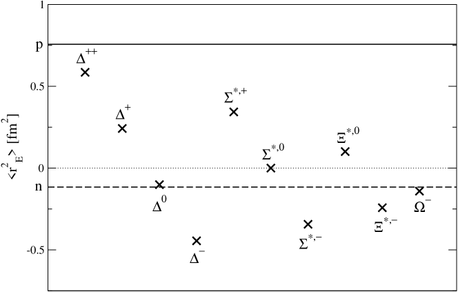
Figure 2: The charge radii of the decuplet baryons in $\chi$PT. The contribution from counterterms has been set to zero. The radii (squared) here come from the one-loop diagrams only and are plotted in units of fm². For reference we have shown both the proton and neutron charge radii (solid and dashed lines, respectively).

III.2 Q$\chi$PT

The calculation of the charge radii and electromagnetic moments can be correspondingly executed for Q$\chi$PT. The operators in Eqs. (27), (29) and (31) contribute, however, their low-energy coefficients cannot be matched onto QCD. Therefore we annotate them with a “Q”. The loop contributions encountered in $\chi$PT and PQ$\chi$PT above no longer contribute because in Q$\chi$PT $A^{T}_{X}=0$ for all decuplet states $T$. This can be readily seen in two ways. The quenched limit of the coefficients in Table 1 makes immediate the vanishing of $A_{X}^{T}$. Alternately one can consider the relevant quark flow diagrams with only valence quarks in loops. Due to the symmetric nature of $T^{ijk}$, these loops are completely canceled by their ghostly counterparts. For the charge radii, there are no additional diagrams to consider at this order from singlet hairpin interactions. Thus in Q$\chi$PT, the charge radii have the form

$$<r_{E}^{2}>=Q\left(\frac{2\mu_{c}^{Q}-1}{M_{B}^{2}}+\frac{\mathbb{Q}_{c}^{Q}+6c_{c}^{Q}}{{\Lambda}_{\chi}^{2}}\right),$$ (38)

where the dependence on the quark mass enters at the next order.

Figure 3: Hairpin diagrams that give contributions of the form $\sim\mu_{o}^{2}\log m_{q}$ to decuplet electromagnetic moments in Q$\chi$PT. The square at the photon vertex represents the relevant operators from Eqs. (27), (29), and (III.2).

Additional terms of the form $\mu_{0}^{2}\log m_{q}$ involving hairpins Labrenz and Sharpe (1996); Savage (2002a) do contribute to the electromagnetic moments as they are of the same order in the chiral expansion. As explained in Chow (1998), the axial hairpins do not contribute. In the diagrams shown in Fig. 3, one sees that there are contributions from the electromagnetic moments of the decuplet and octet baryons as well as their transition moments. These interactions are described by the operators in Eqs. (27) and (29) (now with quenched coefficients) along with

$${\mathcal{L}} = \frac{ie}{2M_{B}}\left\{\mu_{\alpha}^{Q}\left({\overline{{\mathcal{B}}}}[S^{\mu},S^{\nu}]{\mathcal{B}}{\mathcal{Q}}\right)+\mu_{\beta}^{Q}\left({\overline{{\mathcal{B}}}}[S^{\mu},S^{\nu}]{\mathcal{Q}}{\mathcal{B}}\right)\right\}F_{\mu\nu}$$

$$+\sqrt{\frac{3}{2}}\mu_{T}^{Q}\frac{ie}{2M_{B}}\left[\left({\overline{{\mathcal{B}}}}S^{\mu}{\mathcal{Q}}{\mathcal{T}}^{\nu}\right)+\text{h.c.}\right]F_{\mu\nu}+\sqrt{\frac{3}{2}}\mathbb{Q}_{T}^{Q}\frac{e}{{\Lambda}_{\chi}^{2}}\left[\left({\overline{{\mathcal{B}}}}S^{\{\mu}{\mathcal{Q}}{\mathcal{T}}^{\nu\}}\right)+\text{h.c.}\right]v^{\alpha}\partial_{\mu}F_{\nu{\alpha}}.$$

It is easier to work with the combinations $\mu_{D}^{Q}$ and $\mu_{F}^{Q}$ defined by

$$\mu_{\alpha}^{Q}=\frac{2}{3}\mu_{D}^{Q}+2\mu_{F}^{Q}\quad\text{and}\;\;\mu_{\beta}^{Q}=-\frac{5}{3}\mu_{D}^{Q}+\mu_{F}^{Q}.$$ (40)

To calculate the quenched electromagnetic moments, we also need the hairpin wavefunction renormalization diagrams shown in Fig. 1. These along with the diagrams in Fig. 3 are economically expressed in terms of the function

$$I(m_{1},m_{2},{\Delta}_{1},{\Delta}_{2},\mu) =\frac{Y(m_{1},{\Delta}_{1},\mu)+Y(m_{2},{\Delta}_{2},\mu)-Y(m_{1},{\Delta}_{2},\mu)-Y(m_{2},{\Delta}_{1},\mu)}{(m_{1}^{2}-m_{2}^{2})({\Delta}_{1}-{\Delta}_{2})}$$

$$=-i\frac{16\pi^{2}}{3}\int\frac{d^{D}k}{(2\pi)^{D}}\frac{k^{2}-(k\cdot v)^{2}}{(k^{2}-m_{1}^{2})(k^{2}-m_{2}^{2})(k\cdot v-{\Delta}_{1})(k\cdot v-{\Delta}_{2})},$$ (41)

where

$$Y(m,{\Delta},\mu)={\Delta}\left(m^{2}-\frac{2}{3}{\Delta}^{2}\right)\log\frac{m^{2}}{\mu^{2}}+\frac{2}{3}m({\Delta}^{2}-m^{2})\mathcal{R}\left(\frac{{\Delta}}{m}\right)$$ (42)

and we have kept only non-analytic contributions. The following shorthands are convenient

$$I_{\eta_{q}\eta_{q^{\prime}}} =I(m_{\eta_{q}},m_{\eta_{q^{\prime}}},0,0,\mu),$$

$$I^{{\Delta}}_{\eta_{q}\eta_{q^{\prime}}} =I(m_{\eta_{q}},m_{\eta_{q^{\prime}}},{\Delta},0,\mu),$$

$$I^{{\Delta}{\Delta}}_{\eta_{q}\eta_{q^{\prime}}} =I(m_{\eta_{q}},m_{\eta_{q^{\prime}}},{\Delta},{\Delta},\mu).$$ (43)

Specific limits of the function $I_{\eta_{q}\eta_{q^{\prime}}}$ appear in Savage (2002a). The wavefunction renormalization factors arising from hairpin diagrams can then be expressed as

$$Z=1-\frac{\mu_{o}^{2}}{16\pi^{2}f^{2}}\sum_{XX^{\prime}}\left[\frac{1}{2}(\mathcal{C}^{Q})^{2}C_{XX^{\prime}}I_{XX^{\prime}}+\frac{5}{9}(\mathcal{H}^{Q})^{2}B_{XX^{\prime}}I^{{\Delta}{\Delta}}_{XX^{\prime}}\right].$$ (44)

Table 2: The SU$(3)$ coefficients $B_{XX^{\prime}}$ and $C_{XX^{\prime}}$ in Q$\chi$PT.

	$B_{XX^{\prime}}$			$C_{XX^{\prime}}$
	$\quad\eta_{u}\eta_{u}$	$\quad\eta_{u}\eta_{s}$	$\quad\eta_{s}\eta_{s}$	$\quad\eta_{u}\eta_{u}$	$\quad\eta_{u}\eta_{s}$	$\quad\eta_{s}\eta_{s}$
$\Delta^{++},\Delta^{+},\Delta^{0},\Delta^{-}$	$1$	$0$	$0$	$0$	$0$	$0$
$\Sigma^{*,+},\Sigma^{*,0},\Sigma^{*,-}$	$\frac{4}{9}$	$\frac{4}{9}$	$\frac{1}{9}$	$\frac{2}{9}$	$-\frac{4}{9}$	$\frac{2}{9}$
$\Xi^{*,0},\Xi^{*,-}$	$\frac{1}{9}$	$\frac{4}{9}$	$\frac{4}{9}$	$\frac{2}{9}$	$-\frac{4}{9}$	$\frac{2}{9}$
$\Omega^{-}$	$0$	$0$	$1$	$0$	$0$	$0$

The coefficients $B_{XX^{\prime}}$ and $C_{XX^{\prime}}$ are listed in Table 2. The sum in Eq. (44) is over $XX^{\prime}=\eta_{u}\eta_{u}$, $\eta_{u}\eta_{s}$, $\eta_{s}\eta_{s}$. Combining these factors with the tree-level contributions and including the corrections from the diagrams in Fig. 3, we arrive at the quenched decuplet magnetic moment

$$\mu = 2\mu_{c}^{Q}QZ+\frac{\mu_{o}^{2}}{16\pi^{2}f^{2}}\sum_{XX^{\prime}}\left[\frac{1}{2}(Q\mu_{F}^{Q}+{\alpha}\mu_{D}^{Q})(\mathcal{C}^{Q})^{2}C_{XX^{\prime}}I_{XX^{\prime}}\right]$$ (45)

$$+\frac{\mu_{o}^{2}}{16\pi^{2}f^{2}}\sum_{XX^{\prime}}\left[\frac{22}{27}(\mathcal{H}^{Q})^{2}\mu_{c}^{Q}B_{XX^{\prime}}QI^{{\Delta}{\Delta}}_{XX^{\prime}}-\frac{2}{9}\mathcal{C}^{Q}\mathcal{H}^{Q}\mu_{T}^{Q}D_{XX^{\prime}}I^{\Delta}_{XX^{\prime}}\right]$$

and the quenched electric quadrupole moment

$$\mathbb{Q} = -2Q\left(\mu_{c}^{Q}+\mathbb{Q}_{c}^{Q}\frac{2M_{B}^{2}}{{\Lambda}_{\chi}^{2}}\right)Z-\frac{\mu_{o}^{2}}{16\pi^{2}f^{2}}\frac{M_{B}^{2}}{{\Lambda}_{\chi}^{2}}\sum_{XX^{\prime}}\left(\frac{8}{3}\mathcal{C}^{Q}\mathcal{H}^{Q}\mathbb{Q}_{T}^{Q}D_{XX^{\prime}}I^{\Delta}_{XX^{\prime}}\right)$$

$$-\frac{\mu_{o}^{2}}{16\pi^{2}f^{2}}\sum_{XX^{\prime}}\left[(\mathcal{H}^{Q})^{2}\left(\frac{2}{9}\mu_{c}^{Q}+\frac{4}{9}\mathbb{Q}_{c}^{Q}\frac{M_{B}^{2}}{{\Lambda}_{\chi}^{2}}\right)QB_{XX^{\prime}}I^{{\Delta}{\Delta}}_{XX^{\prime}}-\frac{2}{3}\mathcal{C}^{Q}\mathcal{H}^{Q}\mu_{T}^{Q}D_{XX^{\prime}}I^{\Delta}_{XX^{\prime}}\right].$$

In Eq. (45) the required values for the constant ${\alpha}$ are: ${\alpha}_{\Sigma^{*,+}},{\alpha}_{\Sigma^{*,0}},{\alpha}_{\Sigma^{*,-}},{\alpha}_{\Xi^{*,-}}=\frac{1}{3}$ and ${\alpha}_{\Xi^{*,0}}=-\frac{2}{3}$. The coefficients $D_{XX^{\prime}}$ are listed in Table 3. If a particular decuplet state is not listed, the value of $D_{XX^{\prime}}$ is zero for all singlet pairs $XX^{\prime}$.

Table 3: The SU$(3)$ coefficients $D_{XX^{\prime}}$ in Q$\chi$PT. Decuplet states not listed have $D_{XX^{\prime}}=0$.

	$D_{XX^{\prime}}$
	$\quad\eta_{u}\eta_{u}$	$\quad\eta_{u}\eta_{s}$	$\quad\eta_{s}\eta_{s}$
$\Sigma^{*,+}$	$\frac{2}{9}$	$-\frac{1}{9}$	$-\frac{1}{9}$
$\Sigma^{*,0}$	$\frac{1}{9}$	$-\frac{1}{18}$	$-\frac{1}{18}$
$\Xi^{*,0}$	$\frac{1}{9}$	$\frac{1}{9}$	$-\frac{2}{9}$

The above expressions can be used to properly extrapolate quenched lattice data to the physical pion mass. For example, the expression for the quenched magnetic moments for the ${\Delta}$ baryons [Eq. (45)] reduces to

$$\mu=2Q\mu_{c}^{Q}\left(1-\frac{4}{27}\,\frac{\mu_{o}^{2}}{16\pi^{2}f^{2}}(\mathcal{H}^{Q})^{2}I^{{\Delta}{\Delta}}_{\eta_{u}\eta_{u}}\right).$$ (47)

In the above expression we need

$$I^{{\Delta}{\Delta}}_{XX}=\log\frac{m_{X}^{2}}{\mu^{2}}-\frac{{\Delta}m_{X}}{{\Delta}^{2}-m_{X}^{2}}{\mathcal{R}}\left(\frac{{\Delta}}{m_{X}}\right)+\dots.$$ (48)

where the ellipses denote terms analytic in $m_{X}$. Utilizing a least squares analysis and using the values $\mu=1$ GeV and ${\Delta}=270$ MeV , we extrapolate the quenched lattice data Leinweber et al. (1992) to the physical pion mass and find for the ${\Delta}$ resonances

$$\mu=2.89\,Q\;[\mu_{N}].$$ (49)

This is in contrast to the value $\mu\approx 2.49\,Q\;[\mu_{N}]$ found from carrying out a $\chi$PT-type extrapolation Cloet et al. (2003). Notice that for many of the decuplet states, in particular the ${\Delta}$ baryons, the quenched magnetic moments and electric quadrupole moments are proportional to the charge $Q$ (unlike the $\chi$PT and PQ$\chi$PT results). This elucidates the trends seen in the quenched lattice data Leinweber et al. (1992).

IV Conclusions

We have calculated the electromagnetic moments and charge radii for the SU($3$) decuplet baryons in the isospin limit of PQ$\chi$PT and also derived the result for the baryon quartet away from the isospin limit for the $SU(2)$ chiral Lagrangian. The $q^{2}$ dependence of decuplet form factors at one-loop appears in Appendix A. We have also calculated the Q$\chi$PT results.

Knowledge of the low-energy behavior of QQCD and PQQCD is crucial to properly extrapolate lattice calculations from the quark masses used on the lattice to those in nature. For the quenched approximation, where the quark determinant is replaced by unity, one uses Q$\chi$PT to do this extrapolation. QQCD, however, has no known connection to QCD. Observables calculated in QQCD are often found to be more divergent in the chiral limit than those in QCD. This behavior is due to new operators included in the QQCD Lagrangian, which are non-existent in QCD. For the decuplet baryons’ electromagnetic moments and charge radii such operators enter at NNLO in the chiral expansion. Hence, formally our NLO result is not more divergent than its QCD counterpart. This, however, does not mean that our result is free of quenching artifacts. While the expansions about the chiral limit for QCD and QQCD charge radii are formally similar, $<r^{2}>\sim{\alpha}+{\beta}\log m_{Q}+\dots$, the QQCD result consists entirely of quenched oddities: for all decuplet baryons, diagrams that have bosonic or fermionic mesons running in loops completely cancel so that ${\beta}=0$. In other words, the quenched decuplet charge radii have the behavior $<r^{2}>\sim{\alpha}+\dots$ and the result is actually independent of $m_{Q}$ at this order. For the quenched decuplet magnetic moments and electric quadrupole moments, expansions about the chiral limit are again formally similar: $\mu\sim{\alpha}+{\beta}\log m_{Q}+\gamma\sqrt{m_{Q}}+\ldots$ and $\mathbb{Q}\sim{\alpha}+{\beta}\log m_{Q}+\ldots$. However, quenching forces $\gamma=0$ and both ${\beta}$’s arise from singlet contributions involving the parameter $\mu_{o}$, which is of course absent in QCD. Thus the leading non-analytic quark mass dependence that remains for these observables is entirely a quenched peculiarity.

PQQCD, on the other hand, is free of such eccentric behavior. The formal behavior of the electromagnetic observables in the chiral limit has the same form as in QCD. Moreover, there is a well-defined connection to QCD and one can reliably extrapolate lattice results down to the quark masses of reality. The low-energy constants appearing in PQQCD are the same as those in QCD and by fitting them in PQ$\chi$PT one can make predictions for QCD. Our PQ$\chi$PT result will enable the proper extrapolation of PQQCD lattice simulations of the decuplet electromagnetic moments and charge radii and we hope it encourages such simulations in the future.

Appendix A The $q^{2}$ dependence of decuplet form factors

For reference, we provide the $q^{2}$ dependence of the decuplet electromagnetic form factors defined in Section III at one-loop order in the chiral expansion. To do so we define the function

$$P_{X}(x,q^{2})=\sqrt{1-\frac{x(1-x)q^{2}}{m_{X}^{2}}}.$$ (50)

Then we have

$$F_{1}(q^{2}) = Q\left(1-\frac{\mu_{c}q^{2}}{2M_{B}^{2}}-\frac{\mathbb{Q}_{\text{c}}q^{2}}{2{\Lambda}_{\chi}^{2}}+\frac{c_{c}q^{2}}{{\Lambda}_{\chi}^{2}}\right)$$

$$-\frac{3+\mathcal{C}^{2}}{16\pi^{2}f^{2}}\sum_{X}A_{X}\left[\frac{q^{2}}{6}\log\frac{m_{X}^{2}}{\mu^{2}}-2m_{X}^{2}\int_{0}^{1}dx\;P^{2}_{X}(x,q^{2})\log P_{X}(x,q^{2})\right]$$

$$-\frac{\mathcal{H}^{2}}{24\pi^{2}f^{2}}\sum_{X}A_{X}\Bigg{\{}\frac{11}{36}q^{2}\log\frac{m_{X}^{2}}{\mu^{2}}+\frac{5}{3}{\Delta}m_{X}{\mathcal{R}}\left(\frac{{\Delta}}{m_{X}}\right)$$

$$\phantom{GWB}-\int_{0}^{1}dx\Bigg{[}\frac{10}{3}\left(\frac{m_{X}^{2}}{2}-{\Delta}^{2}-\frac{11}{10}x(1-x)q^{2}\right)\log P_{X}(x,q^{2})$$

$$\phantom{anidiot}+{\Delta}m_{X}P_{X}(x,q^{2})\left(\frac{5}{3}+\frac{x(1-x)q^{2}}{{\Delta}^{2}-m_{X}^{2}P^{2}_{X}(x,q^{2})}\right){\mathcal{R}}\left(\frac{\Delta}{m_{X}P_{X}(x,q^{2})}\right)\Bigg{]}\Bigg{\}},$$

$$F_{2}(q^{2}) = 2\mu_{c}Q-\frac{\mathcal{C}^{2}M_{B}}{8\pi f^{2}}\sum_{X}A_{X}m_{X}\int_{0}^{1}dx\;P_{X}(x,q^{2})+\frac{M_{B}\mathcal{H}^{2}}{36\pi^{2}f^{2}}\sum_{X}A_{X}\Bigg{\{}\Delta\log\frac{m_{X}^{2}}{\mu^{2}}$$ (52)

$$\phantom{indeed}+\int_{0}^{1}dx\Bigg{[}2{\Delta}\log P_{X}(x,q^{2})-m_{X}P_{X}(x,q^{2}){\mathcal{R}}\left(\frac{\Delta}{m_{X}P_{X}(x,q^{2})}\right)\Bigg{]}\Bigg{\}},$$

and

$$G_{1}(q^{2}) = 4Q\left(\mu_{c}+\mathbb{Q}_{c}\frac{2M_{B}^{2}}{{\Lambda}_{\chi}^{2}}\right)-\frac{M_{B}^{2}\mathcal{C}^{2}}{2\pi^{2}f^{2}}\sum_{X}A_{X}\left[\frac{1}{6}\log\frac{m_{X}^{2}}{\mu^{2}}+\int_{0}^{1}dx\,2x(1-x)\log P_{X}(x,q^{2})\right]$$ (53)

$$+\frac{2M_{B}^{2}\mathcal{H}^{2}}{9\pi^{2}f^{2}}\sum_{X}A_{X}\Bigg{\{}\frac{1}{6}\log\frac{m_{X}^{2}}{\mu^{2}}+\int_{0}^{1}dx\,x(1-x)\Bigg{[}2\log P_{X}(x,q^{2})$$

$$\phantom{gfhjhgjhghg}-\frac{\Delta m_{X}P_{X}(x,q^{2})}{\Delta^{2}-m^{2}_{X}P^{2}_{X}(x,q^{2})}{\mathcal{R}}\left(\frac{\Delta}{m_{X}P_{X}(x,q^{2})}\right)\Bigg{]}\Bigg{\}}.$$

Appendix B ${\Delta}$ electromagnetic properties in $SU(2)$ flavor with non-degenerate quarks

In this Section, we consider the case of $SU(2)$ flavor and calculate the electromagnetic moments and charge radii of the delta quartet. We keep the up and down valence quark masses non-degenerate and similarly for the sea-quarks. Thus the quark mass matrix reads $m_{Q}^{SU(2)}=\text{diag}(m_{u},m_{d},m_{j},m_{l},m_{u},m_{d})$. Defining ghost and sea quark charges is constrained only by the restriction that QCD be recovered in the limit of appropriately degenerate quark masses. Thus the most general form of the charge matrix is

$${\mathcal{Q}}^{SU(2)}=\text{diag}\left(\frac{2}{3},-\frac{1}{3},q_{j},q_{l},q_{j},q_{l}\right).$$ (54)

The symmetry breaking pattern is assumed to be $SU(4|2)_{L}\otimes SU(4|2)_{R}\otimes U(1)_{V}\longrightarrow SU(4|2)_{V}\otimes U(1)_{V}$. The baryon field assignments are analogous to the case of $SU(3)$ flavor. The nucleons are embedded as

$${\mathcal{B}}_{ijk}=\frac{1}{\sqrt{6}}\left({\epsilon}_{ij}N_{k}+{\epsilon}_{ik}N_{j}\right),$$ (55)

where the indices $i,j$ and $k$ are restricted to $1$ or $2$ and the $SU(2)$ nucleon doublet is defined as

$$N=\left(\begin{matrix}p\\ n\end{matrix}\right)$$ (56)

The decuplet field ${\mathcal{T}}_{ijk}$, which is totally symmetric, is normalized to contain the $\Delta$-resonances $T_{ijk}={\mathcal{T}}_{ijk}$ with $i$, $j$, $k$ restricted to 1 or 2. Our states are normalized so that ${\mathcal{T}}_{111}={\Delta}^{++}$. The construction of the octet and decuplet baryons containing one sea or one ghost quark is analogous to the $SU(3)$ flavor case Beane and Savage (2002a) and we will not repeat it here.

The free Lagrangian for ${\mathcal{B}}$ and ${\mathcal{T}}$ is the one in Eq. (15) (with the parameters having different numerical values than the $SU(3)$ case). The connection to QCD is detailed in Beane and Savage (2002a). Similarly, the Lagrangian describing the interaction of the ${\mathcal{B}}$ and ${\mathcal{T}}$ with the pseudo-Goldstone bosons is the one in Eq. (18). Matching it to the familiar one in QCD (by restricting the ${\mathcal{B}}_{ijk}$ and ${\mathcal{T}}_{ijk}$ to the $qqq$ sector),

$${\mathcal{L}}=g_{{\Delta}N}\left({\overline{T}}{}^{kji}_{\nu}A_{il}^{\nu}N_{j}{\epsilon}_{kl}+\text{h.c}\right)+2g_{{\Delta}{\Delta}}{\overline{T}}{}^{\nu}_{kji}S_{\mu}A^{\mu}_{il}T_{\nu,ljk}+2g_{X}{\overline{T}}{}^{\nu}_{kji}S_{\mu}T_{\nu,ijk}\text{tr}(A^{\mu}),$$ (57)

one finds at tree-level ${\mathcal{C}}=-g_{{\Delta}N}$ and $\mathcal{H}=g_{{\Delta}{\Delta}}$, with $g_{X}=0$. The leading tree-level operators which contribute to ${\Delta}$ electromagnetic properties are the same as in Eqs. (27), (29), and (31), of course the low-energy constants have different values.

Table 4: The SU$(2)$ coefficients $A_{X}^{T}$ in $\chi$PT and PQ$\chi$PT.

	$\chi$PT	PQ$\chi$PT
	$\pi^{\pm}$	$uu$	$ud$	$dd$	$ju$	$lu$	$jd$	$ld$
$\Delta^{++}$	$1$	$-\frac{2}{3}+q_{j}$	$\frac{1}{3}+q_{l}$	$0$	$\frac{2}{3}-q_{j}$	$\frac{2}{3}-q_{l}$	$0$	$0$
$\Delta^{+}$	$\frac{1}{3}$	$-\frac{4}{9}+\frac{2}{3}q_{j}$	$\frac{1}{3}q_{j}+\frac{2}{3}q_{l}$	$\frac{1}{9}+\frac{1}{3}q_{l}$	$\frac{4}{9}-\frac{2}{3}q_{j}$	$\frac{4}{9}-\frac{2}{3}q_{l}$	$-\frac{1}{9}-\frac{1}{3}q_{j}$	$-\frac{1}{9}-\frac{1}{3}q_{l}$
$\Delta^{0}$	$-\frac{1}{3}$	$-\frac{2}{9}+\frac{1}{3}q_{j}$	$-\frac{1}{3}+\frac{2}{3}q_{j}+\frac{1}{3}q_{l}$	$\frac{2}{9}+\frac{2}{3}q_{l}$	$\frac{2}{9}-\frac{1}{3}q_{j}$	$\frac{2}{9}-\frac{1}{3}q_{l}$	$-\frac{2}{9}-\frac{2}{3}q_{j}$	$-\frac{2}{9}-\frac{2}{3}q_{l}$
$\Delta^{-}$	$-1$	$0$	$-\frac{2}{3}+q_{j}$	$\frac{1}{3}+q_{l}$	$0$	$0$	$-\frac{1}{3}-q_{j}$	$-\frac{1}{3}-q_{l}$

Evaluating the ${\Delta}$ electromagnetic properties at NLO in the chiral expansion yields expressions identical in form to those above Eqs. (34), (35), and (37) with the SU$(2)$ identifications made for $\mathcal{C}$ and $\mathcal{H}$ above. The SU$(2)$ coefficients $A_{X}^{T}$ appear in Table 4 for particular ${\Delta}$–resonance states $T$. In the table, we have listed values corresponding to the loop meson that has mass $m_{X}$ for both $\chi$PT and PQ$\chi$PT. Again, the $\chi$PT coefficients can be used to find the ${\Delta}$-resonance charge radii in two-flavor QCD. These have not been previously calculated.

References

• Mergell et al. (1996) P. Mergell, U. G. Meissner, and D. Drechsel, Nucl. Phys. A596, 367 (1996), eprint hep-ph/9506375.
• Hammer et al. (1996) H. W. Hammer, U.-G. Meissner, and D. Drechsel, Phys. Lett. B385, 343 (1996), eprint hep-ph/9604294.
• Gayou et al. (2002) O. Gayou et al. (Jefferson Lab Hall A), Phys. Rev. Lett. 88, 092301 (2002), eprint nucl-ex/0111010.
• Hagiwara et al. (2002) K. Hagiwara et al. (Particle Data Group), Phys. Rev. D66, 010001 (2002).
• Bosshard et al. (1991) A. Bosshard et al., Phys. Rev. D44, 1962 (1991).
• Lopez Castro and Mariano (2002) G. Lopez Castro and A. Mariano, Nucl. Phys. A697, 440 (2002), eprint nucl-th/0010045.
• Kotulla et al. (2002) M. Kotulla et al., Phys. Rev. Lett. 89, 272001 (2002), eprint nucl-ex/0210040.
• Leinweber et al. (1992) D. B. Leinweber, T. Draper, and R. M. Woloshyn, Phys. Rev. D46, 3067 (1992), eprint hep-lat/9208025.
• Morel (1987) A. Morel, J. Phys. (France) 48, 1111 (1987).
• Sharpe (1992) S. R. Sharpe, Phys. Rev. D46, 3146 (1992), eprint [http://arXiv.org/abs]hep-lat/9205020.
• Bernard and Golterman (1992a) C. W. Bernard and M. Golterman, Nucl. Phys. Proc. Suppl. 26, 360 (1992a).
• Bernard and Golterman (1992b) C. W. Bernard and M. F. L. Golterman, Phys. Rev. D46, 853 (1992b), eprint [http://arXiv.org/abs]hep-lat/9204007.
• Golterman (1994) M. F. L. Golterman, Acta Phys. Polon. B25, 1731 (1994), eprint [http://arXiv.org/abs]hep-lat/9411005.
• Sharpe and Zhang (1996) S. R. Sharpe and Y. Zhang, Phys. Rev. D53, 5125 (1996), eprint [http://arXiv.org/abs]hep-lat/9510037.
• Labrenz and Sharpe (1996) J. N. Labrenz and S. R. Sharpe, Phys. Rev. D54, 4595 (1996), eprint [http://arXiv.org/abs]hep-lat/9605034.
• Booth (1994) M. J. Booth (1994), eprint [http://arXiv.org/abs]hep-ph/9412228.
• Kim and Kim (1998) M. Kim and S. Kim, Phys. Rev. D58, 074509 (1998), eprint hep-lat/9608091.
• Savage (2002a) M. J. Savage, Nucl. Phys. A700, 359 (2002a), eprint nucl-th/0107038.
• Arndt (2003) D. Arndt, Phys. Rev. D67, 074501 (2003), eprint hep-lat/0210019.
• Dong et al. (2003) S. J. Dong et al. (2003), eprint hep-lat/0304005.
• Arndt and Tiburzi (2003) D. Arndt and B. C. Tiburzi (2003), eprint hep-lat/0307003.
• Bernard and Golterman (1994) C. W. Bernard and M. F. L. Golterman, Phys. Rev. D49, 486 (1994), eprint [http://arXiv.org/abs]hep-lat/9306005.
• Sharpe (1997) S. R. Sharpe, Phys. Rev. D56, 7052 (1997), eprint [http://arXiv.org/abs]hep-lat/9707018.
• Golterman and Leung (1998) M. F. L. Golterman and K.-C. Leung, Phys. Rev. D57, 5703 (1998), eprint [http://arXiv.org/abs]hep-lat/9711033.
• Sharpe and Shoresh (2000a) S. R. Sharpe and N. Shoresh, Nucl. Phys. Proc. Suppl. 83, 968 (2000a), eprint [http://arXiv.org/abs]hep-lat/9909090.
• Sharpe and Shoresh (2001a) S. R. Sharpe and N. Shoresh, Int. J. Mod. Phys. A16S1C, 1219 (2001a), eprint [http://arXiv.org/abs]hep-lat/0011089.
• Sharpe and Shoresh (2000b) S. R. Sharpe and N. Shoresh, Phys. Rev. D62, 094503 (2000b), eprint [http://arXiv.org/abs]hep-lat/0006017.
• Sharpe and Shoresh (2001b) S. R. Sharpe and N. Shoresh, Phys. Rev. D64, 114510 (2001b), eprint [http://arXiv.org/abs]hep-lat/0108003.
• Shoresh (2001) N. Shoresh (2001), Ph.D. thesis, UMI-30-36529.
• Savage (2002b) M. J. Savage, Phys. Rev. D65, 034014 (2002b), eprint [http://arXiv.org/abs]hep-ph/0109190.
• Chen and Savage (2002) J.-W. Chen and M. J. Savage, Phys. Rev. D65, 094001 (2002), eprint [http://arXiv.org/abs]hep-lat/0111050.
• Beane and Savage (2002a) S. R. Beane and M. J. Savage, Nucl. Phys. A709, 319 (2002a), eprint hep-lat/0203003.
• Savage (2002c) M. J. Savage (2002c), eprint hep-lat/0208022.
• Leinweber (2002) D. B. Leinweber (2002), eprint hep-lat/0211017.
• LAT (a) URL http://www.jlab.org/~dgr/lhpc/march00.pdf.
• LAT (b) URL http://www.jlab.org/~dgr/lhpc/sdac_proposal_final.pdf.
• Beane and Savage (2003) S. R. Beane and M. J. Savage, Phys. Rev. D67, 054502 (2003), eprint hep-lat/0210046.
• Beane and Savage (2002b) S. R. Beane and M. J. Savage, Phys. Lett. B535, 177 (2002b), eprint hep-lat/0202013.
• Arndt et al. (2003) D. Arndt, S. R. Beane, and M. J. Savage (2003), eprint nucl-th/0304004.
• Jenkins and Manohar (1991a) E. Jenkins and A. V. Manohar, Phys. Lett. B255, 558 (1991a).
• Jenkins and Manohar (1991b) E. Jenkins and A. V. Manohar (1991b), talk presented at the Workshop on Effective Field Theories of the Standard Model, Dobogoko, Hungary, Aug 1991.
• Balantekin et al. (1981) A. B. Balantekin, I. Bars, and F. Iachello, Phys. Rev. Lett. 47, 19 (1981).
• Balantekin and Bars (1981) A. B. Balantekin and I. Bars, J. Math. Phys. 22, 1149 (1981).
• Balantekin and Bars (1982) A. B. Balantekin and I. Bars, J. Math. Phys. 23, 1239 (1982).
• Golterman and Pallante (2002) M. Golterman and E. Pallante, Nucl. Phys. Proc. Suppl. 106, 335 (2002), eprint [http://arXiv.org/abs]hep-lat/0110183.
• Butler et al. (1994) M. N. Butler, M. J. Savage, and R. P. Springer, Phys. Rev. D49, 3459 (1994), eprint hep-ph/9308317.
• Banerjee and Milana (1996) M. K. Banerjee and J. Milana, Phys. Rev. D54, 5804 (1996), eprint hep-ph/9508340.
• Buchmann and Lebed (2000) A. J. Buchmann and R. F. Lebed, Phys. Rev. D62, 096005 (2000), eprint hep-ph/0003167.
• Buchmann et al. (2002) A. J. Buchmann, J. A. Hester, and R. F. Lebed, Phys. Rev. D66, 056002 (2002), eprint hep-ph/0205108.
• Buchmann and Lebed (2003) A. J. Buchmann and R. F. Lebed, Phys. Rev. D67, 016002 (2003), eprint hep-ph/0207358.
• Cohen (2003) T. D. Cohen, Phys. Lett. B554, 28 (2003), eprint hep-ph/0210278.
• Nozawa and Leinweber (1990) S. Nozawa and D. B. Leinweber, Phys. Rev. D42, 3567 (1990).
• Jenkins et al. (1993) E. Jenkins, M. E. Luke, A. V. Manohar, and M. J. Savage, Phys. Lett. B302, 482 (1993), eprint hep-ph/9212226.
• Chow (1998) C.-K. Chow, Phys. Rev. D57, 6762 (1998), eprint hep-ph/9711375.
• Cloet et al. (2003) I. C. Cloet, D. B. Leinweber, and A. W. Thomas, Phys. Lett. B563, 157 (2003), eprint hep-lat/0302008.