KANAZAWA-03-17     
ITEP-LAT-2003-12     
Entropy of monopoles from percolating cluster in quenched SU(2) QCD

Abstract

The length distribution and the monopole action of the infrared monopole clusters are studied numerically in quenched SU(2) QCD. We determine the effective entropy of the monopole currents which turns out to be a descending function of the blocking scale, indicating that the effective degrees of freedom of the extended monopoles are getting smaller as the blocking scale increases.

1 INTRODUCTION

The dual superconductor picture [1] of the QCD vacuum is based on the existence of Abelian monopoles which appear naturally in an Abelian gauge. There are various indications that the monopoles are responsible for the color confinement (for a review, see Ref. [2]). One of the most important results is the observation of the monopole condensate in the confinement phase [3, 4].

The monopole trajectories form clusters. Typically, each lattice configuration contains many finite-sized (ultraviolet) clusters and one large percolating (infrared) cluster [5, 6, 7]. The IR cluster – which occupies the whole lattice – represents the monopole condensate [5]. The tension of the confining string gets a dominant contribution from the IR cluster [6]. In the deconfinement phase the IR cluster disappears [5, 6], as expected.

The UV and IR monopole clusters were studied previously in Refs. [6, 7, 8, 9, 10]. Below we investigate the action and length distribution of the infrared monopole cluster for various lattice sizes and scales $b$ at which the magnetic charge is defined. Using the action and length distribution we investigate the entropy of the IR clusters.

2 MODEL

In our simulations we use the Wilson action, $S(U)=-\frac{\beta}{2}\,{\mathrm{Tr}}U_{P}$. We work in the Maximal Abelian (MA) gauge [11]. The Abelian gauge field, $\theta$, is determined as a phase the diagonal component of the $SU(2)$ link variable, $\theta_{\mu}(s)=\arg\,U^{11}_{\mu}(s)$. The Abelian field strength, $\theta_{\mu\nu}(s)\in(-4\pi,4\pi)$, is decomposed into two parts, $\theta_{\mu\nu}(s)=\bar{\theta}_{\mu\nu}(s)+2\pi m_{\mu\nu}(s)$, where $\bar{\theta}_{\mu\nu}(s)\in[-\pi,\pi)$ is interpreted as the electromagnetic flux through the plaquette and $m_{\mu\nu}(s)$ can be regarded as a number of the Dirac strings piercing the plaquette.

The elementary monopole currents are defined as follows [12], $k_{\mu}(s)=1/2\epsilon_{\mu\nu\rho\sigma}\partial_{\nu}m_{\rho\sigma}(s+\hat{\mu})$, where $\partial$ is the forward lattice derivative. To study the monopole charges at various scales we use the $n^{3}$ extended monopole construction [5],

$$k_{\mu}^{(n)}(s)=\!\!\sum_{i,j,l=0}^{n-1}\!\!k_{\mu}(ns+(n-1)\hat{\mu}+i\hat{\nu}+j\hat{\rho}+l\hat{\sigma}).$$

The extended monopole is defined on a sublattice with the spacing $b=na$, where $a$ is the spacing of the original lattice. Both elementary and extended monopole charges are conserved and quantized.

We used the standard Monte–Carlo procedure to generate 1000-3000 configurations of the gauge field for each value of $\beta=2.1\sim 2.6$. To fix the MA gauge we used either the usual iterative algorithm (for $24^{4}$ and $48^{4}$ lattices) or the Simulated Annealing method [13] with five Gribov copies (for $32^{4}$ lattice).

3 MONOPOLE ACTION

To get the monopole action we integrate out all degrees of freedom but the monopole ones. Following Ref. [3] we generate the SU(2) configurations, fix the MA gauge, then get the configurations of the IR monopole clusters as it was described in the previous section. Then we use the inverse Monte–Carlo method to get the monopole action.

The monopole action can be represented [3, 15] as a sum of the $n$–point ($n\geq 2$) operators $S_{i}$:

$$S_{{\mathrm{mon}}}[k]=\sum_{i}f_{i}S_{i}[k]\,,\vspace{-2mm}$$

where $f_{i}$ are the coupling constants. We adopt only the two–point interactions in the monopole action ($i.e.$ interactions of the form $S_{i}\sim k_{\mu}(s)k_{\mu^{\prime}}(s^{\prime})$). A detailed description of the $S_{i}[k]$ interactions can be found in Ref. [16].

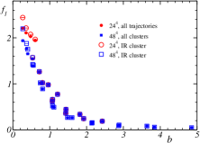
Figure 1: The self–interaction coupling $f_{1}$ $vs.$ $b$.

One can find that the monopole action is proportional with a good accuracy to the length of the monopole loop, $S_{{\mathrm{mon}}}=fL+const$. The dominant term in the monopole action corresponds to the most local self-interaction of the monopole currents, $S_{1}[k]=\sum_{s,\mu}k^{2}_{\mu}(s)$. We compare the parameter $f_{1}$ for the monopole action of the IR cluster and for the action associated with the whole monopole ensemble in Figure 1.

One can notice that the coupling constant $f_{1}$ shows scaling for large $b=na$ in agreement with Ref. [3]. This coupling is independent of the lattice volume and for large blocking scales $b$ the type of the ensemble (the IR cluster or the whole ensemble) is not essential for determination of $f_{1}$. However, at small $b$ values, $b\sqrt{\sigma}\lesssim 0.5$, the type of the lattice ensemble becomes important.

4 LENGTH DISTRIBUTION

The distribution of the ultraviolet clusters was studied both numerically [7, 10] and analytically [9, 14]. The distribution can be described by a power law $D_{UV}\propto L^{-\tau}$, where the power $\tau$ is very close to 3, Ref. [7]. This behaviour indicates that the monopoles in UV clusters are randomly walking objects [9]. In our simulations we are concentrated on the IR cluster because the IR cluster is important for the confinement of quarks.

The length distribution function, $D(L)$, is proportional to the weight with which the particular trajectory of the length $L$ contributes to the partition function. From the previous section it is clear that monopole action contributes to $D(L)$ in a form of an exponential factor, $\propto e^{-fL}$. The entropy of the monopole trajectory also contributes to the monopole length distribution. The entropy contribution is proportional to $\mu^{L}$ (with $\mu>0$) for sufficiently large monopole lengths, $L$. Thus the distribution of the monopole trajectories in infinite volume must be described by the function

$$D^{IR}_{\inf}(L)\propto\mu^{L}\cdot e^{-f\,L}=e^{\gamma L}\,,\quad\gamma=\ln\mu-f\,.$$ (1)

In this equation we neglect a power-law prefactor which is essential for the distribution of the ultraviolet clusters. In the finite volume there appears a finite–volume suppression factor and the total distribution can be described as a Gaussian [16]:

$$D^{IR}(L)=const.\,\exp\{-\alpha(b,V)L^{2}+\gamma(b)L\}\,.$$ (2)

The peak of this distribution, $L_{max}=\gamma(b)/2\,\alpha(b,V)$, is expected to be proportional to the volume of the system, $V$, to insure the finiteness of the IR monopole density, $\rho_{IR}=L_{max}/V$, in the thermodynamic limit, $V\to\infty$. Thus we conclude that $\alpha(b,V)=A(b)/V$, where $A(b)$ is a certain function. Therefore in the thermodynamic limit the parameter $\alpha$ vanishes and the distribution (2) is reduced to Eq.(1), as expected.

To get the monopole entropy we need to know the parameter $\gamma$, Eq. (1). We fit the monopole loops distributions by the function (2) and use the bootstrap method to estimate the statistical errors. We obtain that the parameter $\gamma$ — shown in Figure 2 — scales with $b=n\cdot a$ and is independent on the volume of the system.

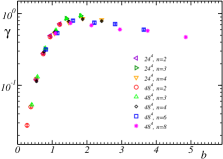
Figure 2: The fitting parameter $\gamma$ as functions $b$ for various lattice volumes and blocking steps, $n$.

5 MONOPOLE ENTROPY

The knowledge of the distribution and the monopole action allows us to determine the entropy of the monopole currents. According to Eq. (1), $\mu=e^{\gamma+f}$. If the monopoles make a simple random walk on a $4D$ hypercubic lattice then we get $\mu=7$ since there are seven choices at each site for the monopole current to go further.

The entropy factor $\mu$ is shown in Figure 3. It scales with $b$ and is independent of the volume of the lattice. Note that in a small $b$ region $\mu>7$ because the monopole action can not be reliably described by the quadratic terms only [15].

At large $b$ the entropy factor is smaller than seven. We have fitted the entropy by a function:

$$\mu^{\mathrm{fit}}=\mu_{\infty}+C\,\mu^{-q}\,,$$ (3)

where $\mu_{\infty}$, $C$ and $q$ are the fitting parameters. The fit gives $\mu_{\infty}=1.6(4)$, $C=1.7(5)$ and $q=1.2(2)$. Fixing $q=1$ in Eq. (3) we get $\mu_{\infty}=1.15(25)$ and $C=2.2(1)$. The corresponding best fit curves are shown in Figure 3.

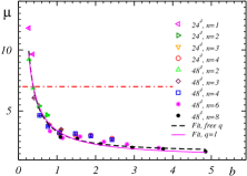
Figure 3: Entropy factor $\mu$ $vs.$ $b$. The lines represent the fits by Eq. (3).

The fact that the asymptotic value of the entropy is very close to the unity in the large $b$ limit may have a simple explanation. A monopole with a large blocking size $b$ behaves as a classical object and its motion is no more a simple random walk. The predominant motion of the large–$b$ monopole is close to a straight line.

References

- [1] G. ’t Hooft, in High Energy Physics, ed. A. Zichichi, EPS International Conference, Palermo (1975); S. Mandelstam, Phys. Rept. 23 (1976) 245.
- [2] T. Suzuki, Nucl. Phys. Proc. Suppl. 30 (1993) 176; M. N. Chernodub, M. I. Polikarpov, in ”Confinement, duality, and nonperturbative aspects of QCD”, Ed. by P. van Baal, Plenum Press, p. 387, hep-th/9710205; R.W. Haymaker, Phys. Rept. 315 (1999) 153.
- [3] H. Shiba, T. Suzuki, Phys. Lett. B 351 (1995) 519.
- [4] N. Arasaki et al, Phys. Lett. B 395 (1997) 275; M.Chernodub, M.I.Polikarpov, A.I.Veselov, Phys.Lett.B 399 (1997) 267; Nucl. Phys. Proc. Suppl. 49 (1996) 307; A. Di Giacomo, G. Paffuti, Phys. Rev. D 56 (1997) 6816.
- [5] T.L. Ivanenko, A.V. Pochinsky, M.I. Polikarpov, Phys. Lett. B 252 (1990) 631.
- [6] S. Kitahara, Y. Matsubara, T. Suzuki, Progr. Theor. Phys. 93 (1995) 1.
- [7] A. Hart, M. Teper, Phys. Rev., B58 (1998) 014504.
- [8] P. Y. Boyko, M. I. Polikarpov, V. I. Zakharov, hep-lat/0209075.
- [9] M.Chernodub, V.I.Zakharov,hep-th/0211267
- [10] V.G. Bornyakov et al, hep-lat/0305021.
- [11] A. S. Kronfeld et al, Phys. Lett. B 198, 516 (1987); Nucl. Phys. B 293, 461 (1987).
- [12] T. A. DeGrand, D. Toussaint, Phys. Rev. D 22 (1980) 2478.
- [13] G. S. Bali et al, Phys. Rev. D 54 (1996) 2863.
- [14] V. I. Zakharov, hep-ph/0202040
- [15] M. N. Chernodub et al, Phys. Rev. D 62 (2000) 094506; hep-lat/9902013.
- [16] M. N. Chernodub, et al, hep-lat/0306001.