BI-TP 2003/19
Oktober 2003

Correlation lengths and scaling functions
in the three-dimensional $O(4)$ model
J. Engels, L. Fromme and M. Seniuch

Fakultät für Physik, Universität Bielefeld, D-33615 Bielefeld, Germany

Abstract

We investigate numerically the transverse and longitudinal correlation lengths of the three-dimensional $O(4)$ model as a function of the external field $H$. From our data we calculate the scaling function of the transverse correlation length, and that of the longitudinal correlation length for $T>T_{c}$. We show that the scaling functions do not only describe the critical behaviours of the correlation lengths but encompass as well the predicted Goldstone effects, in particular the $H^{-1/2}$-dependence of the transverse correlation length for $T<T_{c}$. In addition, we determine the critical exponent $\delta=4.824(9)$ and several critical amplitudes from which we derive the universal amplitude ratios $R_{\chi}=1.084(18),~{}Q_{c}=0.431(9),~{}Q_{2}^{T}=4.91(8),~{}Q_{2}^{L}=1.265(24)$ and $U_{\xi}^{c}=1.99(1)$. The last result supports a relation between the longitudinal and transverse correlation functions, which was conjectured to hold below $T_{c}$ but seems to be valid also at $T_{c}$.

PACS : 64.10.+h; 75.10.Hk; 05.50+q

Keywords: Correlation length; $O(4)$ model; Goldstone modes; Scaling function; Universal amplitude ratios

 
E-mail addresses: engels@physik.uni-bielefeld.de, fromme@physik.uni-bielefeld.de,
seniuch@physik.uni-bielefeld.de

1 Introduction

In $O(N)$ spin models with $N>1$ two types of correlation lengths appear. They govern the exponential decay of the correlation functions of the transverse and longitudinal spin components, defined relative to the external field $\vec{H}$. Like in the case of the magnetization and the susceptibilities, the behaviour of the correlation lengths in the critical region is described by asymptotic scaling functions, critical exponents and amplitudes, which characterise the underlying universality class. These quantities are of general interest. In addition, there are predictions [1, 2] for the correlation lengths, which are related to the presence of massless Goldstone modes [3, 4] and are still untested. The measurement of the correlation lengths as functions of the field $H$ enables us to verify these predictions and to determine the critical parameters and scaling functions. We have chosen the three-dimensional $O(4)$ model to carry out this program for the following reasons. Firstly, this model is of importance for quantum chromodynamics (QCD) with two degenerate light-quark flavours at finite temperature, because it is believed [5]-[9] to belong to the same universality class as QCD at its chiral transition in the continuum limit. Secondly, the $H$-dependent model has already been investigated in some detail by Monte Carlo methods, in particular the critical behaviours of the magnetization [10, 11] and susceptibilities. In addition the corresponding Goldstone-mode effects have been verified [11].

The specific model which we study here is the standard $O(4)$-invariant nonlinear $\sigma$-model, which is defined by

$$\beta\,{\cal H}\;=\;-J\,\sum_{<{\vec{x}},{\vec{y}}>}\vec{\phi}_{\vec{x}}\cdot\vec{\phi}_{\vec{y}}\;-\;{\vec{H}}\cdot\,\sum_{{\vec{x}}}\vec{\phi}_{\vec{x}}\;,$$ (1)

where ${\vec{x}}$ and ${\vec{y}}$ are nearest-neighbour sites on a three-dimensional hypercubic lattice, and $\vec{\phi}_{\vec{x}}$ is a four-component unit vector at site ${\vec{x}}$. It is convenient to decompose the spin vector $\vec{\phi}_{\vec{x}}$ into longitudinal (parallel to the magnetic field $\vec{H}$) and transverse components

$$\vec{\phi}_{\vec{x}}\;=\;\phi_{\vec{x}}^{\parallel}\vec{e}_{H}+\vec{\phi}_{\vec{x}}^{\perp}~{},\quad{\rm with}\quad\vec{e}_{H}=\vec{H}/H~{}.$$ (2)

The order parameter of the system, the magnetization $M$, is then the expectation value of the lattice average $\phi^{\parallel}$ of the longitudinal spin components

$$M\;=\;\langle\>\frac{1}{V}\sum_{{\vec{x}}}\phi_{\vec{x}}^{\parallel}\>\rangle\;=\;\langle\,\phi^{\parallel}\,\rangle~{}.$$ (3)

Here $V=L^{3}$ and $L$ is the number of lattice points per direction. There are two types of susceptibilities. The longitudinal susceptibility is the usual derivative of the magnetization, whereas the transverse susceptibility corresponds to the fluctuation per component of the lattice average $\vec{\phi}^{\perp}$ of the transverse spin components

$$\chi_{L}\!\! \!=\! \!\!{\partial M\over\partial H}\;=\;V(\langle\,\phi^{\parallel 2}\,\rangle-M^{2})~{},$$ (4)

$$\chi_{T}\!\! \!=\! \!\!{V\over 3}\langle\,\vec{\phi}^{\perp 2}\,\rangle\;=\;{M\over H}~{}.$$ (5)

The expectation value $\langle\,\vec{\phi}^{\perp}\,\rangle$ is of course zero. The connected two-point correlation functions of the longitudinal and transverse spins are defined by

$$G_{L}({\vec{x}})\!\! \!=\! \!\!\langle\>\phi^{\parallel}_{\vec{x}}\phi^{\parallel}_{0}\>\rangle-M^{2}~{},$$ (6)

$$G_{T}({\vec{x}})\!\! \!=\! \!\!{1\over 3}\langle\>\vec{\phi}^{\perp}_{\vec{x}}\cdot\vec{\phi}^{\perp}_{0}\>\rangle~{}.$$ (7)

They are related to the susceptibilities by

$$\chi_{L,T}\;=\;\sum_{{\vec{x}}}G_{L,T}({\vec{x}})~{}.$$ (8)

For all temperatures $T$ (the coupling $J$ acts here as inverse temperature, i. e. $J=1/T$) and fields $H$, except on the coexistence line $H=0,T<T_{c}$ and at the critical point, the large distance behaviour of these correlation functions is determined by the respective exponential correlation lengths $\xi_{L,T}$

$$G_{L,T}({\vec{x}})\sim\exp(-|\vec{x}|/\xi_{L,T})~{}.$$ (9)

On the coexistence line, where the correlation functions decay according to a power law, it is still possible to define a transverse correlation length [12] from the so-called stiffness constant. We do however not consider this option here.

1.1 Goldstone-Mode Effects

The spontaneous breaking of the rotational symmetry for temperatures below the critical point gives rise to the so-called spin waves: slowly varying long-wavelength spin configurations, whose energies may be arbitrarily close to the ground-state energy - the massless Goldstone modes [13]. For $H\rightarrow 0$ the magnetization $M$ below $T_{c}$ attains a finite value, the spontaneous magnetization $M(T,0)$ (here and in the following we assume always that $H\geq 0$, so that $M(T,0)>0$). The transverse susceptibility $\chi_{T}=M/H$, which is directly related to the fluctuation of the Goldstone modes, diverges therefore as $H^{-1}$ when $H\rightarrow 0$ for all $T<T_{c}$. It is non-trivial that also the longitudinal susceptibility $\chi_{L}$ is diverging on the coexistence curve. The predicted divergence in three dimensions is [14]

$$\chi_{L}(T<T_{c},H)\sim H^{-1/2}~{}.$$ (10)

From a phenomenological spin wave analysis and the behaviour of the transverse susceptibility $\chi_{T}$ Fisher and Privman [1] arrived at the conclusion that the bulk correlation length, which they identify with the transverse correlation length, diverges also when $H\rightarrow 0$ as

$$\xi_{T}(T<T_{c},H)\sim H^{-1/2}~{}.$$ (11)

In fact, this connection between the behaviours of the correlation length and the respective susceptibility, namely

$$\xi_{T}^{2}\sim\chi_{T},$$ (12)

is what one usually expects [15]. For instance, when masses are defined from the corresponding inverse susceptibilities,

$$m^{2}=\chi^{-1}~{},$$ (13)

one would anticipate that $m\sim\xi^{-1}$. In QCD, the transverse mass corresponds [7] to the pion mass, $m_{T}=m_{\pi}$, and the longitudinal one to the sigma mass, $m_{L}=m_{\sigma}$. According to Ref. [1], the relation equivalent to Eq. (12), $\xi_{L}^{2}\sim\chi_{L}$, does not hold for the longitudinal fluctuations at long wavelengths, because they are driven by the transverse fluctuations and the bulk correlation length also sets the scale of the decay of $G_{L}({\vec{x}})$. This statement is substantiated by the well-known relation [1, 2] between the longitudinal and transverse correlation functions at zero field, $T<T_{c}$ and large distances $|{\vec{x}}|$

$$G_{L}({\vec{x}})\approx{1\over 2}(N-1)\left[{G_{T}({\vec{x}})\over M}\right]^{2}~{},$$ (14)

where in our case $N=4$. One expects that the relation is still valid for small non-zero fields $H$ near the phase boundary in the region of exponential decay. That implies a factor of 2 between the correlation lengths.

The rest of the paper is organized as follows. First we discuss the critical behaviours of the observables and the universal scaling functions, which we want to calculate. In Section 3 we describe some details of our simulations and the way we determine the correlation lengths. Section 4 serves to find the critical amplitudes, which are needed for the normalizations and the universal ratios. In the following Section 5 we discuss the scaling functions which we obtain from our data. The Goldstone effect on the transverse correlation length is demonstrated in Section 6. Subsequently we investigate the $H$-dependence of the correlation lengths in the high temperature phase. We close with a summary and the conclusions.

2 Critical Behaviour and Scaling Functions

In the thermodynamic limit ($V\rightarrow\infty$) the observables show power law behaviour close to $T_{c}$. It is described by critical amplitudes and exponents of the reduced temperature $t=(T-T_{c})/T_{c}$. The scaling laws at $H=0$ are for

the magnetization

$$M\;=\;B(-t)^{\beta}\quad{\rm for~{}}t<0~{},$$ (15)

the longitudinal susceptibility

$$\chi_{L}\;=\;C^{+}t^{-\gamma}\quad{\rm for~{}}t>0~{},$$ (16)

and since for $H=0,t>0$ the correlation lengths coincide $\xi_{T}=\xi_{L}=\xi$ (like the susceptibilities)

$$\xi\;=\;\xi^{+}t^{-\nu}\quad{\rm for~{}}t>0~{}.$$ (17)

On the critical line $T=T_{c}$ or $t=0$ we have for $H>0$ the scaling laws

$$M\;=\;B^{c}H^{1/\delta}\quad{\rm or}\quad H\;=\;D_{c}M^{\delta}~{},$$ (18)

$$\chi_{L}\;=\;C^{c}H^{1/\delta-1}\quad{\rm with}\quad C^{c}\;=\;B^{c}/\delta~{},$$ (19)

and for the correlation lengths

$$\xi_{L,T}\;=\;\xi^{c}_{L,T}H^{-\nu_{c}}~{},\quad\nu_{c}\;=\;\nu/\beta\delta~{}.$$ (20)

We assume the following hyperscaling relations among the critical exponents to be valid

$$\gamma\;=\;\beta(\delta-1),\quad d\nu\;=\;\beta(1+\delta),\quad 2-\eta\;=\;\gamma/\nu~{}.$$ (21)

As a consequence only two critical exponents are independent. Because of the hyperscaling relations and the already implicitly assumed equality of the critical exponents above and below $T_{c}$ one can construct a multitude of universal amplitude ratios [12] (see also the discussion in Ref. [16]). The following list of ratios contains those which we will determine here

$$\!\!\!R_{\chi}\;=\;C^{+}D_{c}B^{\delta-1}~{},\,\quad U_{\xi}^{c}\;\;=\;\xi^{c}_{T}/\xi^{c}_{L}~{},$$ (22)

$$Q_{c}\;=\;B^{2}(\xi^{+})^{d}/C^{+}~{},\quad Q_{2}^{L,T}\;=\;(\xi^{c}_{L,T}/\xi^{+})^{\gamma/\nu}C^{+}/C^{c}~{}.$$ (23)

The critical behaviour of the magnetization in the vicinity of $T_{c}$ is more generally described by the magnetic equation of state. In its Widom-Griffiths form it is given by [17, 18]

$$y\;=\;f(x)~{},$$ (24)

where

$$y\equiv h/M^{\delta}~{},\quad x\equiv\bar{t}/M^{1/\beta}~{}.$$ (25)

The variables $\bar{t}$ and $h$ are the normalized reduced temperature $\bar{t}=tT_{c}/T_{0}$ and magnetic field $h=H/H_{0}$, which are chosen such as to fulfill the standard normalization conditions

$$f(0)\;=\;1~{},\quad f(-1)\;=\;0~{},$$ (26)

which imply

$$M(t=0)=h^{1/\delta}\quad{\rm and}\quad H_{0}=D_{c}~{},$$ (27)

$$M(h=0)=(-\bar{t}\;)^{\beta}\quad{\rm and}\quad T_{0}=B^{-1/\beta}T_{c}~{}.$$ (28)

Possible dependencies on irrelevant scaling fields and exponents are however not taken into account in Eq. (24), the function $f(x)$ is universal. Another way to express the dependence of the magnetization on $\bar{t}$ and $h$ is

$$M\;=\;h^{1/\delta}f_{G}(\bar{t}/h^{1/\beta\delta})~{},$$ (29)

where $f_{G}$ is again a universal scaling function. The two forms (24) and (29) are of course equivalent. The function $f_{G}(z)$ and its argument $z$ are related to $x$ and $y$ by

$$f_{G}=y^{-1/\delta}~{},\quad z\equiv\bar{t}/h^{1/\beta\delta}=xy^{-1/\beta\delta}~{}.$$ (30)

Correspondingly the normalization conditions (26) translate into

$$f_{G}(0)\;=\;1~{},\quad{\rm and}\quad f_{G}(z){\raisebox{-4.30554pt}{$\stackrel{{\scriptstyle\displaystyle\longrightarrow}}{{\scriptstyle z\rightarrow-\infty}}$}}(-z)^{\beta}~{}.$$ (31)

Since the susceptibility $\chi_{L}$ is the derivative of $M$ with respect to $H$ we obtain from Eq. (29)

$$\chi_{L}={\partial M\over\partial H}={h^{1/\delta-1}\over H_{0}}f_{\chi}(z)~{},$$ (32)

with

$$f_{\chi}(z)={1\over\delta}\left(f_{G}(z)-{z\over\beta}f_{G}^{\prime}(z)\right)~{}.$$ (33)

For $H\to 0$ at fixed $t>0$, that is for $z\rightarrow\infty$, the leading asymptotic term of $f_{\chi}$ is determined by Eq. (16)

$$f_{\chi}(z)\;{\raisebox{-4.30554pt}{$\stackrel{{\scriptstyle\displaystyle=}}{{\scriptstyle z\rightarrow\infty}}$}}\;C^{+}D_{c}B^{\delta-1}z^{-\gamma}\;=\;R_{\chi}z^{-\gamma}~{}.$$ (34)

For $z\rightarrow\infty$ the leading terms of $f_{G}$ and $f_{\chi}$ are identical, because for $T>T_{c}$ and small magnetic field $M$ is proportional to $H$.

Like for $M$ and $\chi_{L}$ the dependence of the correlation lengths on $\bar{t}$ and $h$ in the critical region and the thermodynamic limit is given in terms of scaling functions $g_{\xi}^{L,T}(z)$ by

$$\xi_{L,T}\;=\;h^{-\nu_{c}}g_{\xi}^{L,T}(z)~{}.$$ (35)

These functions are universal except for a normalization factor. On the critical line $\bar{t}=0$ or $z=0$ we find from (20)

$$g_{\xi}^{L,T}(0)\;=\;\xi^{c}_{L,T}D_{c}^{-\nu_{c}}\;=\;\xi^{c}_{L,T}(B^{c})^{\nu/\beta}~{},$$ (36)

and from (17) the asymptotic behaviour at $z\to\infty$ (which is the same for both correlation lengths),

$$g_{\xi}^{L,T}(z)\;{\raisebox{-4.30554pt}{$\stackrel{{\scriptstyle\displaystyle=}}{{\scriptstyle z\rightarrow\infty}}$}}\;\xi^{+}B^{\nu/\beta}z^{-\nu}~{}.$$ (37)

Indeed, the ratios of the amplitude for $z\to\infty$ in (37) and the $g_{\xi}^{L,T}(0)$ are universal

$${\xi^{+}B^{\nu/\beta}\over\xi^{c}_{L,T}(B^{c})^{\nu/\beta}}\;=\;\left({\delta R_{\chi}\over Q_{2}^{L,T}}\right)^{\nu/\gamma}~{},$$ (38)

whereas the $g_{\xi}^{L,T}(0)$ itself are not. In analogy to the Ising case discussed in Ref. [15] we therefore define two universal scaling functions by

$${\hat{g}}_{\xi}^{L,T}(z)\;=\;g_{\xi}^{L,T}(z)/g_{\xi}^{L,T}(0)~{}.$$ (39)

3 Numerical Details

All our simulations were done on three-dimensional lattices with periodic boundary conditions and linear extensions $L=48,72,96$ and 120. As in Ref. [11] we have used the Wolff single cluster algorithm [19], which was modified to include a non-zero magnetic field [20]. In order to reduce the integrated autocorrelation time $\tau_{int}$ we performed 100-3000 cluster updates between two measurements for $H>0$, such that we obtained $\tau_{int}\mathrel{\hbox to0.0pt{\lower 3.0pt\hbox{$\mathchar 536\relax$}\hss}\raise 2.0pt\hbox{$\mathchar 316\relax$}}3$ for $L=48$ and $\tau_{int}\mathrel{\hbox to0.0pt{\lower 3.0pt\hbox{$\mathchar 536\relax$}\hss}\raise 2.0pt\hbox{$\mathchar 316\relax$}}5$ for $L\geq 72$. For $H=0,T>T_{c}$ and large lattices the number of cluster updates was increased up to 10000. In general we made 20000 measurements for each fixed $H$ and $J$. We use the value for $J_{c}=T_{c}^{-1}=0.93590$ from Ref. [21]. The coupling constant region which we have explored was $0.9\leq J\leq 1.2$, the magnetic field was varied from $H=0$ to $H=0.01$.

3.1 Measurement of the Correlation Lengths

Instead of using correlation functions of the individual spins it is more favourable to consider spin averages over planes and their respective correlation functions. For example, the spin average over the $(x,y)$-plane at position $z$ is defined by

$${\vec{S}}_{z}={1\over L^{2}}\sum_{x,y}\vec{\phi}_{\vec{x}}~{}.$$ (40)

The spin averages have again longitudinal and transverse components

$${\vec{S}}_{z}\;=\;S_{z}^{\parallel}\vec{e}_{H}+{\vec{S}}_{z}^{\perp}~{},$$ (41)

The expectation values of the components are independent of $z$ and equal to those of the respective lattice averages

$$\langle S_{z}^{\parallel}\rangle=\langle\phi^{\parallel}\rangle=M~{},\quad{\rm and}\quad\langle{\vec{S}}_{z}^{\perp}\rangle=\langle\vec{\phi}^{\perp}\rangle=0~{}.$$ (42)

Correspondingly, we define now plane-correlation functions ${\bar{G}}_{L,T}(z)$ by

$${\bar{G}}_{L}(z)\!\! = \!\!L^{2}\left(\langle S_{0}^{\parallel}S_{z}^{\parallel}\rangle-M^{2}\right)$$ (43)

$${\bar{G}}_{T}(z)\!\! = \!\!{L^{2}\over 3}\langle{\vec{S}}_{0}^{\perp}{\vec{S}}_{z}^{\perp}\rangle~{}.$$ (44)

Here, $z$ is the distance between the two planes. Instead of choosing the $z$-direction as normal to the plane one can as well take the $x$- or $y$-directions. Accordingly, we enhance the accuracy of the correlation function data by averaging over all three directions and all possible translations. The correlators are symmetric and periodic functions of the distance $\tau$ between the planes, the factor $L^{2}$ on the right-hand sides of (43) and (44) ensures the relation

$$\chi_{L,T}=\sum_{\tau=0}^{L-1}{\bar{G}}_{L,T}(\tau)~{}.$$ (45)

Like the point-correlation functions in Eq. (9) the plane correlators ${\bar{G}}_{L,T}(\tau)$ decay exponentially. In order to obtain the corresponding exponential correlation length $\xi$ from ${\bar{G}}(\tau)$ we therefore make the ansatz

$${\bar{G}}(\tau)=A\left[\>\exp(-\tau/\xi)+\exp(-(L-\tau)/\xi)\>\right]~{},$$ (46)

and then try to fit the data for the correlation functions in an appropriate $\tau$-range. The ansatz (46) implies of course, that there are no additional excitations contributing to ${\bar{G}}(\tau)$. Inspired by the experiences reported in the Ising case [22, 15], we proceed in the following way. First we calculate an effective correlation length $\xi^{eff}(\tau)$ from (46) using only the correlators at $\tau$ and $\tau+1$. For $\tau\ll L$ this correlation length is approximately given by

$$\xi^{eff}(\tau)={-1\over\ln({\bar{G}}(\tau+1)/{\bar{G}}(\tau))}~{}.$$ (47)

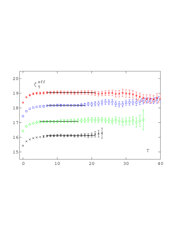
Figure 1: The effective transverse correlation length $\xi^{eff}_{T}$ at $J=0.95$ and $H=0.001$ for $L=48$ (crosses), 72 (diamonds), 96 (squares) and 120 (stars) as a function of $\tau$. The lines show the corresponding $\tau$-ranges where fits to Eq. (46) were performed, their heights the resulting fit values. The data for $L=72,96$ and 120 have been shifted upwards by 1, 2 and 3 for better visibility.

As an example, we show in Fig. 1 a typical result for $\xi^{eff}(\tau)$ at $J=0.95,\,H=0.001$, that is in the low temperature region, from the transverse correlation functions on lattices with $L=48,72,96$ and 120. With increasing $\tau$ also $\xi^{eff}$ increases and eventually reaches a plateau inside its error bars. Most likely, the lower values of $\xi^{eff}$ at small $\tau$ are due to higher excitations. At large distances $\tau$ the resulting $\xi^{eff}$ start to fluctuate when the relative errors of the data become too large. The two limits define an intermediate $\tau$-range where a global fit with the ansatz (46) can be used to estimate the exponential correlation length $\xi$. It is clear, that due to the strong correlations between the values ${\bar{G}}(\tau)$ for different $\tau$, the result from a fit in the whole range of the plateau must be essentially the same as that of one (low) $\tau$-value in the plateau. That is indeed the case: the two estimates for $\xi$ agree within the error bars and the errors themselves are of about the same size, or somewhat larger for the plateau fits.

$J$	$\xi_{T}^{eff}(\tau_{a})$	$\xi_{T}$	$[\tau_{a},\tau_{b}]$	$\xi_{L}^{eff}(\tau_{a})$	$\xi_{L}$	$[\tau_{a},\tau_{b}]$
0.95	16.054(69)	16.080(105)	5-16	-	-	-
0.9359	13.447(46)	13.449(49)	6-21	6.738(55)	6.767(64)	8-17
0.93	11.789(36)	11.813(32)	6-26	7.594(57)	7.647(60)	8-19
0.92	8.563(32)	8.592(26)	3-17	7.705(54)	7.720(60)	4-15

Table 1: Correlation length estimates for different $J$ and $H=0.001$: $\xi^{eff}(\tau_{a})$ is the value at the lower end of the plateau region $[\tau_{a},\tau_{b}]$, $\xi$ the value from fits to the ansatz (46) in the whole plateau region.

Using the latter makes the result less dependent on the special choice of $\tau$, where $\xi^{eff}$ is evaluated, in case the $\xi^{eff}$-values are slightly fluctuating. In order to give an impression of the different $\xi$-estimates, their errors and the respective $\tau$-ranges we show in Table 1 some representative results for $T$ below, at and above $T_{c}$ and $H=0.001$ on a lattice with $L=72$ (at $J=0.92$ with $L=48$).

With our method we found reliable values for the exponential transverse correlation length $\xi_{T}$ at all $T$. In the case of the longitudinal correlation length $\xi_{L}$ the same is true in the high temperature phase $T>T_{c}$. However, at $T_{c}$ and slightly below the critical point at $H>0$ there are already indications for the presence of higher states. Deeper in the low temperature phase it becomes impossible to estimate the longitudinal correlation length: no plateau appears, there is a dense spectrum of states contributing to the longitudinal correlator.

4 Critical Amplitudes and Universal Ratios

In Ref. [11] the spontaneous magnetization $M(T,0)$ was calculated at several temperatures on the coexistence line, taking advantage of the Goldstone effect on $M$. From these results the critical amplitude $B$ of Eq. (15) and the normalization $T_{0}$ could be determined to $B=0.9916(5)$ and $T_{0}=1.093(2)$ using $\beta=0.380$. We use these values in the following. In the same paper the amplitude $B^{c}$ and the critical exponent $\delta$ were determined from fits to the critical behaviour of $M$ on the critical line. Since we have done new simulations on the critical line with higher statistics and at more $H$-values on the larger lattices than in [11] we could improve the analysis with the new magnetization data.

4.1 Results from the Critical Line

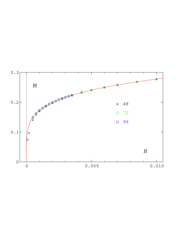
Figure 2: The magnetization $M$ at $T_{c}$ as a function of the magnetic field $H$ for $L=48,72$ and 96. The solid line shows the fit (48).

On the critical isotherm, that is at $T_{c}$, we have measured the magnetization for $H>0$ on lattices with $L=48,72$ and 96. The results are shown in Fig. 2. We observe essentially only for $L=48$ a noticeable finite size dependence close to $H=0$. Like in [11] we have made various fits to the data from the largest lattices in the $H$-interval $[0.00075,\;0.00425]$ with the simple ansatz

$$M\;=\;B^{c}H^{1/\delta}~{}.$$ (48)

The resulting values for the amplitude and the exponent are (with $\chi^{2}/N_{f}\approx 1.7$)

$$B^{c}\;=\;0.721(2)\quad{\rm and}\quad\delta\;=\;4.824(9)~{},$$ (49)

and lead to $D_{c}=H_{0}=4.845(66)$. The solid curve in Fig. 2 shows this fit. It also represents the data at higher magnetic fields very well. From these additional data a marginal negative correction-to-scaling term may be inferred, which is however irrelevant at low $H$. Compared to the corresponding fit in [11], where $\delta\;=\;4.86(1)$, we note that our new result for $\delta$ is closer to the value 4.789(6) from Ref. [23]. The latter value was however deduced from calculations at zero magnetic field. All the other critical exponents which were needed in our calculations have been derived from the hyperscaling relations (21) and $\beta=0.380,\>\delta=4.824\>$. We use therefore

$$\nu=0.7377~{},\quad\gamma=1.4531~{},\quad\nu_{c}=0.4024~{}.$$ (50)

The data for the transverse and longitudinal correlation lengths on the critical line are shown in Fig. 3 (a) and (b). For the transverse correlation length $\xi_{T}$ we find only finite size effects very close to $H=0$.

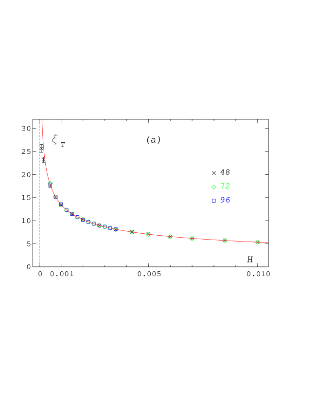
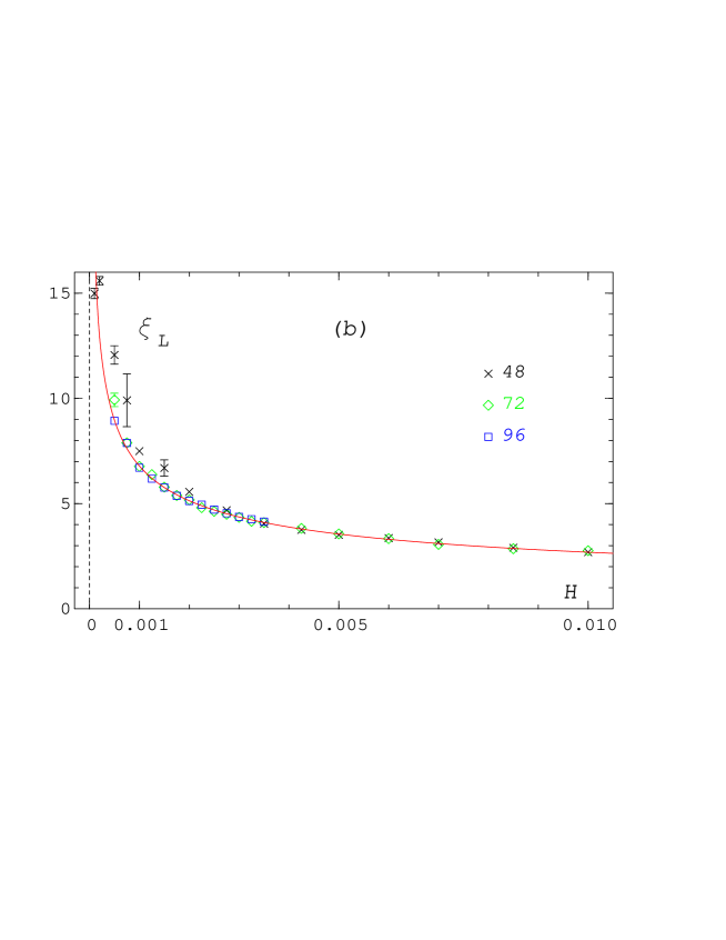
Figure 3: The correlation lengths $\xi_{T}$ (a) and $\xi_{L}$ (b) at $T_{c}$ for $L=48,72$ and 96 as a function of $H$. The lines are the fits (51) with $\xi_{T,L}^{c}$ from (52) and $c_{T,L}=0$.

The longitudinal correlation length $\xi_{L}$ exhibits fluctuations and a systematic deviation to higher $\xi_{L}$-values, when the magnetic field is decreasing. The smaller the lattice, the earlier this behaviour sets in. In order to determine the amplitudes we have fitted our results to the following form with $\omega=0.8$

$$\xi_{T,L}\;=\;\xi_{T,L}^{c}H^{-\nu_{c}}\left(1+c_{T,L}H^{\omega\nu_{c}}\right)~{}.$$ (51)

In both cases we have taken various subsets of the data for the fits in the $H$-interval [0.0005,0.005]. It turned out that the correction terms are zero within their error bars and that fits with $c_{T,L}\equiv 0$ work just as well. The $\chi^{2}/N_{f}$ varies between 0.5 and 0.8 . We find for the amplitudes

$$\xi_{T}^{c}\;=\;0.838(1)~{},\quad\xi_{L}^{c}\;=\;0.421(2)~{}.$$ (52)

As can be seen from Fig. 3 (a) and (b), the corresponding fits describe the data also in the higher $H$-range up to $0.01\>$. The ratio of the two correlation lengths is remarkably close to 2

$$U_{\xi}^{c}\;=\;\xi_{T}^{c}/\xi_{L}^{c}\;=\;1.99(1)~{},$$ (53)

that is, the expectation for the ratio from Eq. (14) close to the coexistence line is fulfilled also at $T_{c}$. A similar observation has been made for the three-dimensional $O(2)$ model [24].

4.2 Results for $T>T_{c}$ and $H=0$

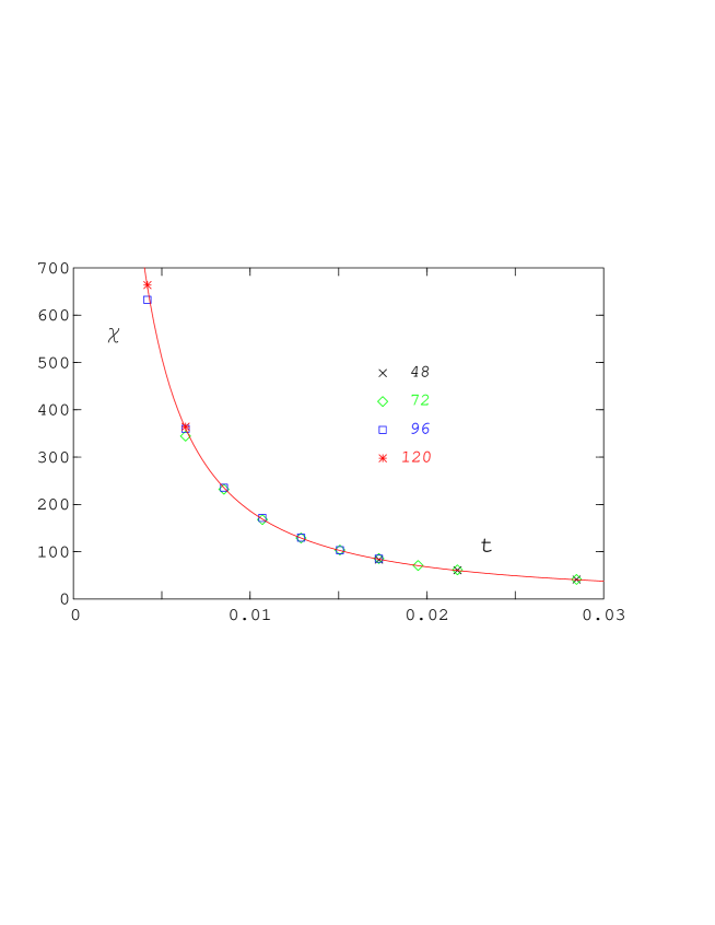
Figure 4: The susceptibility above $T_{c}$ at $H=0$ for $L=48,72,96$ and 120 versus the reduced temperature $t$. The solid line shows the leading term of the fit to Eq. (54).

Our next aim is the determination of the critical amplitudes $C^{+}$ and $\xi^{+}$. To this end we have evaluated the data of the susceptibility and of the correlation length above the critical temperature for $H=0$. The data points for $\chi=\chi_{L}=\chi_{T}$ are plotted in Fig. 4 as a function of $t$. We have made various fits with the ansatz

$$\chi\;=\;C^{+}t^{-\gamma}[1+C_{1}^{+}t^{\omega\nu}]~{},$$ (54)

in the $J$-interval [0.91,0.932], which corresponds to $0.00415\leq t\leq 0.0285$. All fits, including a correction term $\sim C_{1}^{+}$ or not, are compatible with the critical amplitude result

$$C^{+}\>=\>0.231(2)~{}.$$ (55)

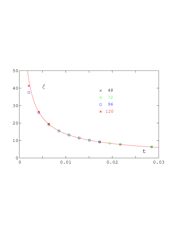
Figure 5: The correlation length $\xi$ above $T_{c}$ at $H=0$ for $L=48,72,96$ and 120 versus $t$. The solid line shows the fit from Eq. (57).

For the correction amplitude we find $C_{1}^{+}=0.14(7)$, and $\chi^{2}/N_{f}$ is in the range $[1.3,1.8]$ . As can be seen in Fig. 4, where only the leading term is plotted, the correction contribution is marginal.

The correlation length data for $H=0$ above the critical temperature are shown in Fig. 5. Like for the susceptibility we have made an ansatz including a correction-to-scaling term

$$\xi=\xi^{+}t^{-\nu}[1+\xi^{+}_{1}t^{\omega\nu}]~{}.$$ (56)

Different fits in the same $J$-interval [0.91, 0.932], which was already used in the case of the susceptibility, lead to the result

$$\xi=0.466(2)t^{-\nu}[1-0.12(4)t^{\omega\nu}]~{},$$ (57)

with a $\chi^{2}/N_{f}$ between 0.8 and 1.2 . The critical amplitude of the correlation length is therefore

$$\xi^{+}=0.466(2)~{}.$$ (58)

4.3 Universal Amplitude Ratios

The critical amplitudes $B^{c},\>\xi^{c}_{L,T},\>C^{+},\>\xi^{+}$, which we have just determined, and $B$ from [11] enable us to fix the necessary normalizations of the scaling functions and in addition we can calculate the universal amplitude ratios defined in Eqs. (22) and (23). The ratio $U_{\xi}^{c}$ has already been discussed. We obtain for the other ratios

$$R_{\chi}=1.084(18)~{},\quad Q_{c}=0.431(9)~{},\quad Q_{2}^{T}=4.91(8)~{},\quad Q_{2}^{L}=1.265(24)~{}.$$ (59)

For the ratio $R_{\chi}$ several alternative values exist: from the parametrization of the equation of state in [11] one gets 1.126(9), from another parametrization in [9] 1.12(11), from the $1/N$-expansion of Oku and Okabe [25] 1.098, and from the $\epsilon$-expansion 1.239 [12]. Our finding for $Q_{c}$ is well in accord with the result 0.44(2) of [9]. We could not find competing values for the ratios $Q_{2}^{L,T}$ in the literature.

5 The Scaling Functions

In Ref. [11] the equation of state in the Widom-Griffiths form was parametrized by a combination of a small-$x$ (low temperature) form $x_{s}(y)$, which was inspired by the approximation of Wallace and Zia [14] close to the coexistence line ($x=-1;~{}y=0$)

$$x_{s}(y)+1\;=\;({\widetilde{c}_{1}}\,+\,{\widetilde{d}_{3}})\,y\,+\,{\widetilde{c}_{2}}\,y^{1/2}\,+\,{\widetilde{d}_{2}}\,y^{3/2}\;,$$ (60)

and a large-$x$ (high temperature) form $x_{l}(y)$ derived from Griffiths’s analyticity condition [18]

$$x_{l}(y)\;=\;a\,y^{1/\gamma}\,+\,b\,y^{(1-2\beta)/\gamma}~{}.$$ (61)

The two parts are interpolated smoothly by the ansatz

$$x(y)\;=\;x_{s}(y)\,\frac{y_{0}^{p}}{y_{0}^{p}+y^{p}}\,+\,x_{l}(y)\,\frac{y^{p}}{y_{0}^{p}+y^{p}}~{},$$ (62)

from which the total scaling function is obtained. Since we have changed the values of $H_{0}$ and of $\delta$ in comparison to Ref. [11], we have redone the corresponding parametrization fits. With the new data we find

$${\widetilde{c}_{1}}\,+\,{\widetilde{d}_{3}}\;=\;0.359(10)~{},\quad{\widetilde{c}_{2}}\;=\;0.666(6)~{},$$ (63)

and ${\widetilde{d}_{2}}=1-({\widetilde{c}_{1}}+{\widetilde{d}_{3}}+{\widetilde{c}_{2}})$ is fixed by the normalization condition $y(0)=1$. The new values for $a$ and $b$ are

$$a\;=\;1.071(4)~{},\quad b\;=\;-0.866(38)~{}.$$ (64)

The interpolation parameters $y_{0}=10.0$ and $p=3$ have been retained unchanged. The modified values of $a$ and $\gamma$ result in a new estimate of $R_{\chi}$

$$R_{\chi}\;=\;a^{\gamma}\;=\;1.105(4)~{},$$ (65)

in nice agreement with the value we obtained in (59) directly from the amplitudes.

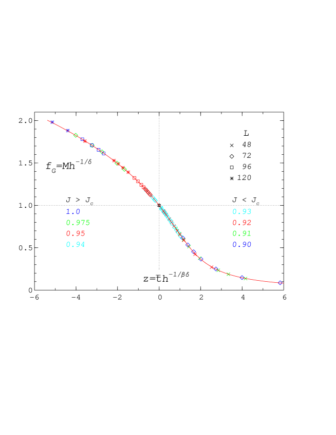
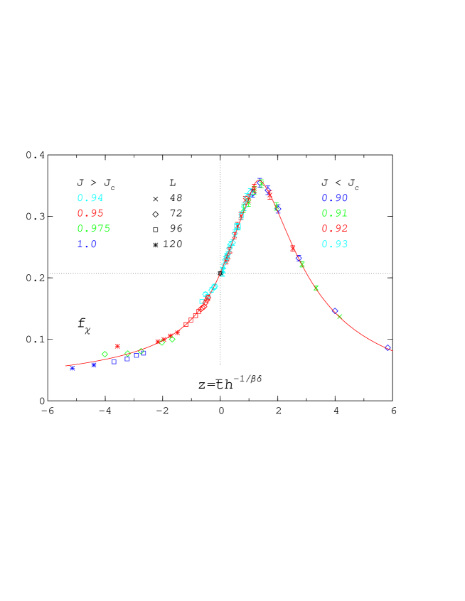
Figure 6: The equation of state: $f_{G}=Mh^{-1/\delta}$ as a function of $z=\bar{t}h^{-1/\beta\delta}$. The solid line shows our parametrization. The numbers refer to the different $J=1/T$-values of the data, the dotted lines cross at the normalization point $f_{G}(0)=1$.

Figure 7: The scaling function $f_{\chi}(z)=\chi_{L}H_{0}h^{1-1/\delta}$ versus $z=\bar{t}h^{-1/\beta\delta}$. The solid line is from our parametrization of the equation of state. The numbers refer to the $J=1/T$-values of the data. The normalization is $f_{\chi}(0)=1/\delta$.

In Fig. 7 we present the results for $f_{G}(z)$ obtained from the magnetization data in the coupling range $0.90\leq J\leq 1.0\>$. At first sight these data are scaling well. Since the data from the coupling $J=1.2$ showed already visible deviations from scaling behaviour we have discarded them. Similarly, limitations were found for the scaling $H$-regions. The data for $f_{G}(z)$ were scaling in the low temperature region only up to $H=0.005$ and in the high temperature region for $J=0.93$ and $J=0.92$ up to $H=0.05$, for $J=0.91$ and $J=0.90$ the scaling $H$-range extended only to $H=0.01$. Only data within these parameter ranges are shown in Fig. 7$\,.$ In the same figure we show the function $f_{G}(z)$, which one obtains with Eq. (30) from our parametrization for $x(y)$. It obviously describes the data quite well. The scaling function $f_{\chi}(z)$ of the susceptibility is connected via Eq. (33) to the scaling function $f_{G}(z)$ of the magnetization. It can therefore be calculated from the parametrization as well. On the other hand we have direct data for $\chi_{L}$ from our simulations which allows for another check of the scaling hypothesis and a comparison to the parametrization. In Fig. 7 we show the respective data for the same $J$-values as in Fig. 7. The data are not as accurate as those for the magnetization. We observe explicit scaling in the high temperature phase ($z>0$), but with decreasing temperature, or larger $-z$, the data are spreading and no longer scaling. In particular the data at the coupling $J=1.0$ seem to be already outside the critical region. For $J=0.975$ and $J=0.95$ it is possible that at very small $H$ (large $-z$) finite size effects are responsible for that behaviour. The other data are coinciding in essence with our parametrization for $z>-3$.

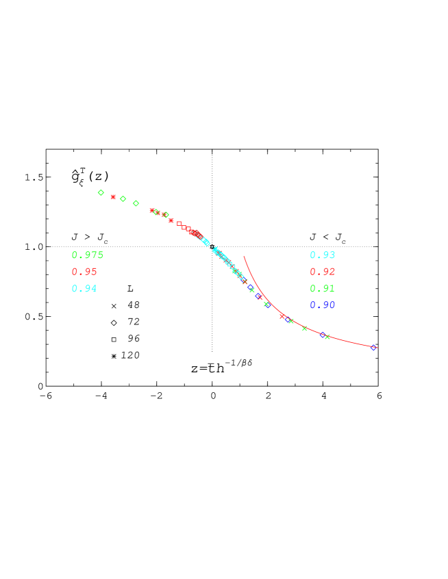
Figure 8: The scaling function of the transverse correlation length $\hat{g}_{\xi}^{T}(z)=\xi_{T}h^{\nu_{c}}/g_{\xi}^{T}(0)$. The solid line is the asymptotic form calculated from Eq. (37). The numbers refer to the different $J=1/T$-values of the data.

5.1 The Scaling Functions of the Correlation Lengths

In Fig. 8 we show the data for the normalized scaling function $\hat{g}_{\xi}^{T}(z)=\xi_{T}h^{\nu_{c}}/g_{\xi}^{T}(0)$. The determination of the transverse correlation length with the method described in Section 3.1 was always possible. In each case a plateau in $\xi^{eff}$ could be found. The data shown in Fig. 8 correspond to the ones presented in Fig. 7 for the scaling function of the susceptibility, apart from the points for $J=1.0\,$, which were clearly outside the scaling region. The normalization was calculated from Eq. (36) and is $g_{\xi}^{T}(0)=0.444(3)$. As in the case of the magnetization and the susceptibility we observe scaling of the correlation length data in a large $z$-range. For $z>0$ we see an early approach to the asymptotic form calculated from Eq. (37). The shape of $\hat{g}_{\xi}^{T}(z)$ is very similar to that of $f_{G}(z)$. It is not by accident that we find this behaviour but it is due to the relation (12) between the transverse correlation length and its susceptibility, which we discussed in Section 1.1$\>.$ We consider therefore the ratio of $\xi_{T}^{2}$ and $\chi_{T}$ and find

$${\xi_{T}^{2}\over\chi_{T}}\;=\;(\xi^{c}_{T})^{2}(B^{c})^{-1}H^{-\eta\nu_{c}}\cdot{(\hat{g}_{\xi}^{T})^{2}\over f_{G}}~{},$$ (66)

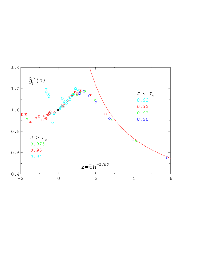
Figure 9: The scaling function of the longitudinal correlation length $\hat{g}_{\xi}^{L}(z)=\xi_{L}h^{\nu_{c}}/g_{\xi}^{L}(0)$. The solid line is obtained from the asymptotic form (37). The numbers refer to the different $J=1/T$-values. The dashed line indicates the peak position of $\chi_{L}$, the symbol notation is as in Fig. 8.

the same relation as in the Ising case [15], execpt that here $f_{\chi}$ is replaced by $f_{G}$, which plays the corresponding part for the transverse correlation length. In the Ising case we found the asymptotic behaviour

$${\hat{g}_{\xi}^{2}\over f_{\chi}}\;{\raisebox{-4.30554pt}{$\stackrel{{\scriptstyle\displaystyle\sim}}{{\scriptstyle z\rightarrow\pm\infty}}$}}\;(\pm z)^{-\eta\nu}~{}.$$ (67)

It is easy to show that $(\hat{g}_{\xi}^{T})^{2}/f_{G}$ for $z\rightarrow+\infty$ is proportional to $z^{-\eta\nu}$. If for $H\rightarrow 0$ the transverse correlation length behaves as $\xi_{T}\sim H^{-1/2}$ - as expected because of the Goldstone effect - then for $z\rightarrow-\infty$ the ratio $(\hat{g}_{\xi}^{T})^{2}/f_{G}$ must be proportional to $(-z)^{-\eta\nu}$, as in the Ising case. The condition for the asymptotic behaviour of the ratio in the broken phase and the $H^{-1/2}$-behaviour of $\xi_{T}$ are thus equivalent.

Assuming the corresponding asymptotic behaviour for $(\hat{g}_{\xi}^{L})^{2}/f_{\chi}$ would imply that $\xi_{L}\sim H^{-1/4}$ for $T<T_{c}$, in contradiction to the expectation of a factor of 2 between the two correlation lengths. The situation in the low temperature region is indeed difficult and as it seems we cannot clarify numerically the status of $\xi_{L}$ there. In Fig. 9 we show our results for the normalized scaling function $\hat{g}_{\xi}^{L}(z)=\xi_{L}h^{\nu_{c}}/g_{\xi}^{L}(0)$, where $g_{\xi}^{L}(0)=0.223(2)$ was determined from Eq. (36). In the high temperature region the longitudinal correlation length could be calculated with sufficient accuracy, the finite size effects were negligible. Approaching the critical temperature ($z=0$) from above, the data become more and more noisy and below $T_{c}$ we are essentially unable to determine $\xi_{L}$ and $\hat{g}_{\xi}^{L}(z)$: if one can find a plateau in $\xi^{eff}$ at all, then the results for different lattice sizes are often very different. In addition scaling is completely lost already for small negative values of $z$. We have therefore only included the data for $z>-2$ in Fig. 9 to show this behaviour. As compared to the transverse scaling function in the high temperature region we have a different functional form, which is similar to that of the scaling function of the longitudinal susceptiblity in Fig. 7. Like in the Ising case, both functions have a peak at about the same $z$-value, which is at $z_{p}\approx 1.335$ in $f_{\chi}$, in accord with the value 1.33(5) found in Ref. [8]. As in Fig. 8 we find an early approach to the asymptotic form given by Eq. (37).

6 The $H$-Dependence of $\xi_{T}$ at Fixed $T<T_{c}$

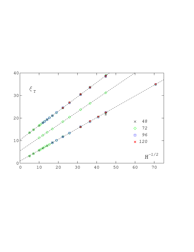
Figure 10: The transverse correlation length as a function of $H^{-1/2}$ for $J=0.95,0.975$ and $1.0\,$. The lowest values are those of $J=0.95$, the highest belong to $J=1.0\,$. For better visibility we have lifted the results for $J=0.975\,(1.0)$ by $5.0\,(10.0)$. The dashed lines represent the straight line fits (68) to the data.

Goldstone-mode effects are expected for all temperatures below $T_{c}$, not only in the critical region, but also there. We have discussed already in the last section, that the shape of the scaling function for the transverse correlation length is explicitly determined in its asymptotic part for $z\rightarrow-\infty$ by the predicted dependency of $\xi_{T}$ on $H^{-1/2}$ for $H\rightarrow 0$. We have tested this prediction by calculating $\xi_{T}$ at three fixed temperatures below $T_{c}$. The data for $\xi_{T}$ are plotted versus $H^{-1/2}$ in Fig. 10 for $J=0.95,0.975$ and $J=1.0\>$. Actually, the same data points from the larger lattices, apart from those for $J=1.0$, had already been included in our scaling plot. We see from Fig. 10 that the data always follow a straight line

$$\xi_{T}\;=\;x_{0}(J)H^{-1/2}+x_{1}(J)~{},$$ (68)

where the slope is slightly increasing with increasing $J$: $x_{0}=0.481(2),0.577(1)$ and 0.637(2) for the three $J$-values. The temperature dependence of $x_{0}$ can be derived from the scaling function by comparing its leading asymptotic behaviour to the $H$-dependence of $\xi_{T}$. If

$$g_{\xi}^{T}(z)\;=\;g_{q}(-z)^{q}+\dots~{},$$ (69)

with $g_{q}$ a constant, then the power $q$ must be $q=\beta\delta/2-\nu$ to lead to the required $H$-dependence for $\xi_{T}$. That implies

$$x_{0}\;=\;g_{q}(-\bar{t})^{q}H_{0}^{1/2}~{},$$ (70)

and since $q=0.1789$ is positive, we have an increase with increasing $J$. We can check the $J$-dependence of the slopes $x_{0}$ by taking ratios

$${x_{0}(J_{1})\over x_{0}(J_{2})}=\left({-\bar{t}_{1}\over-\bar{t}_{2}}\right)^{q}~{}.$$ (71)

For $x_{0}(0.975)/x_{0}(0.95)=1.200(5)$ our formula predicts 1.195, that is rather close to the fit value. For $x_{0}(1.0)/x_{0}(0.975)=1.104(4)$ we get 1.088, a slightly lower result. On the other hand, the data for $J=1.0$ were just outside the scaling region and somewhat higher than the scaling function. The small deviation to a higher ratio is therefore what one expects.

7 The $H$-Dependence of $\xi_{T,L}$ at Fixed $T>T_{c}$

At $H=0$ the correlation lengths in the symmetric phase $(T>T_{c})$ are equal. We have shown the $t$-dependence in Fig. 5. With increasing $H$, however, they differ and $\xi_{T}$ is always bigger than $\xi_{L}$. In Fig. 11 we show the two correlation lengths as a function of $H$ for three different fixed couplings or temperatures: $J=0.92,0.91$, and 0.90. The lattice sizes were $L=48$ and 72. Essentially no finite size effect was found. As expected, the correlation lengths decrease with increasing field from their value at $H=0$. The reduction itself is diminishing with increasing temperatures (decreasing couplings $J=1/T$), the curves become flatter and the difference between the two correlation lengths disappears. This behaviour can be understood from the asymptotic expansions of the scaling functions of the correlation lengths. In the symmetric phase the correlation lengths are even functions of $h$, so that $\xi(h)=\xi(-h)$ (we omit the indices $T$ and $L$ for this discussion). The scaling function $g_{\xi}(z)$ must then have an asymptotic expansion for $z\rightarrow\infty\>(h\rightarrow 0,\bar{t}$ fixed) of the form

$$g_{\xi}(z)\;=\;z^{-\nu}\sum_{n=0}^{\infty}g_{n}z^{-2\Delta n}~{},$$ (72)

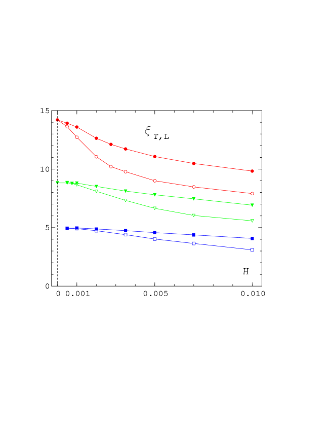
Figure 11: The correlation lengths $\xi_{T}$ (filled symbols) and $\xi_{L}$ (empty symbols) as a function of $H$. The couplings are $J=0.92$ (circles), $J=0.91$ (triangles) and $J=0.90$ (squares). In order to disentangle the different curves we have lifted the results for $J=0.92\,(0.91)$ by 5.0 (2.5). The data are connected by straight lines to guide the eye.

where the $g_{n}$ are constants, $g_{0}=\xi^{+}B^{\nu/\beta}$, and $\Delta=\beta\delta$. This translates into the following $h$-expansion for the correlation length at fixed $\bar{t}$ and small $h$

$$\xi\;=\;(\bar{t})^{-\nu}\sum_{n=0}^{\infty}g_{n}\cdot(\bar{t})^{-2\Delta n}h^{2n}~{}.$$ (73)

For very small magnetic fields $h$ we have

$$\xi\;=\;g_{0}(\bar{t})^{-\nu}+g_{1}(\bar{t})^{-\nu-2\Delta}h^{2}+\dots~{},$$ (74)

and with increasing $\bar{t}$ the $h$-dependence will disappear with a factor $\sim(\bar{t})^{-2\Delta}$ compared to the value at $h=0$.

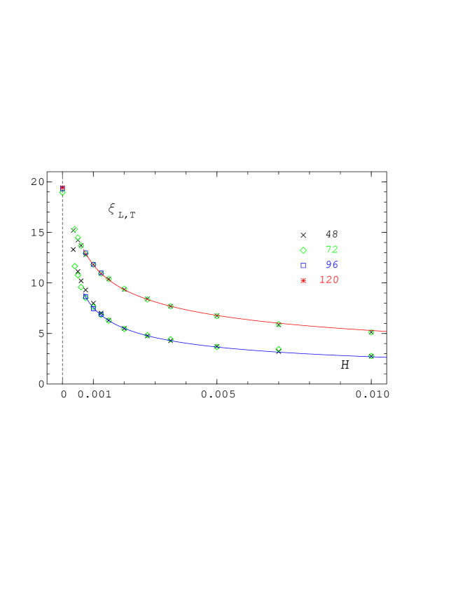
Figure 12: The correlation lengths $\xi_{T}$ (upper set of data) and $\xi_{L}$ (lower set) as a function of $H$ for the coupling $J=0.93$. The lines are fits to Eq. (76) in the interval [0.0006,0.005].

In the neighbourhood of the critical point, where $|z|$ is small (but not $h$), one can expand $g_{\xi}(z)$ in powers of $z$ and obtains

$$\xi\;=\;h^{-\nu_{c}}g_{\xi}(z)\;=\;h^{-\nu_{c}}\left(g_{0}^{c}+g_{1}^{c}z+g_{2}^{c}z^{2}+\dots\right)~{},$$ (75)

with $g_{0}^{c}=\xi^{c}(B^{c})^{\nu/\beta}$. That leads to the following $h$-dependence of $\xi$

$$\xi\;=\;h^{-\nu_{c}}\left(g_{0}^{c}+g_{1}^{c}{\bar{t}}h^{-1/\Delta}+g_{2}^{c}(\bar{t})^{2}h^{-2/\Delta}+\dots\right)~{},$$ (76)

when the temperature is near to the critical point. In Fig. 12 we show as an example the correlation lengths for $J=0.93$, close to $J_{c}=0.93590\>$. We have made fits in the $H$-interval [0.0006,0.005], using only the first two terms in Eq. (76). Obviously these simple fits describe the data quite well in a large range.

8 Summary and Conclusions

In this paper we have investigated the correlation lengths of the three-dimensional $O(4)$ model with Monte Carlo simulations. One of the main objectives was to find the functional dependence of the correlation lengths on the external field at fixed temperature, a second to understand the interplay of the critical behaviour and the effects induced by the massless Goldstone-modes. A main result of our work is the calculation of the scaling function of the transverse correlation length and that of the longitudinal correlation length for $T\geq T_{c}$. In the low temperature phase we were, however, unable to reliably estimate $\xi_{L}$. The reason for that is the rich spectrum of states which contribute to the longitudinal correlators below the critical point. In the simpler Ising model [15], where only one correlation length exists, the influence of higher states [26] complicates the determination of the correlation length below $T_{c}$, but in contrast to the $O(4)$ model it is still possible there.

As we could show, the scaling functions do not only describe the critical behaviours of the correlation lengths, but encompass as well the predicted Goldstone effects. Indeed, in consequence of the relation $\xi_{T}^{2}\sim\chi_{T}$ and the equation $\chi_{T}\,=\,M/H$ for the fluctuation of the transverse spin components, the prediction $\xi_{T}\sim H^{-1/2}$ emerges below $T_{c}$ and leads to a similar functional form of the scaling functions of $\xi_{T}$ and that of the magnetization. In the high temperature phase a similar correspondence exists between the scaling functions of $\xi_{L}$ and that of the longitudinal susceptibility. There both functions have a peak at the same position, a behaviour which was found also in the Ising model [15].

In preparation of the scaling functions we have determined several critical amplitudes of the correlation lengths: $\xi_{T}^{c},\,\xi_{L}^{c}$ and $\xi^{+}$ and in addition also $B^{c}$ and $C^{+}$. As a byproduct we have found the critical exponent $\delta\,=\,4.824(9)$. The critical amplitudes allowed us to directly determine the universal amplitude ratios $R_{\chi},\,Q_{c},\,Q_{2}^{L,T}$ and $U_{\xi}^{c}\,=\,1.99(1)\,$. The latter result is most remarkable, because it confirms a relation between the longitudinal and transverse correlation functions, which was conjectured to hold below $T_{c}$, but seems to be valid also at $T_{c}$. Acknowledgments

We thank Sven Holtmann and Thomas Schulze for their constant interest and assistance during the course of the work. Our work was supported by the Deutsche Forschungsgemeinschaft under Grant No. FOR 339/2-1.

References

- [1] M. E. Fisher and V. Privman, Phys. Rev. B 32 (1985) 447.
- [2] A. L. Patashinskii and V. L. Pokrovskii, Zh. Eksp. Teor. Fiz. 64 (1973) 1445 [Sov. Phys. JETP 37 (1974) 733].
- [3] J. Zinn-Justin, Quantum Field Theory and Critical Phenomena, Clarendon Press, Oxford, 3rd Edition 1996.
- [4] R. Anishetty, R. Basu, N. D. Hari Dass and H. S. Sharatchandra, Int. J. Mod. Phys. A 14 (1999) 3467 [hep-th/9502003].
- [5] R. D. Pisarski and F. Wilczek, Phys. Rev. D 29 (1984) 338.
- [6] F. Wilczek, Int. J. Mod. Phys. A 7 (1992) 3911 [Erratum-ibid. A 7 (1992) 6951].
- [7] K. Rajagopal and F. Wilczek, Nucl. Phys. B 399 (1993) 395 [hep-ph/9210253].
- [8] J. Engels, S. Holtmann, T. Mendes and T. Schulze, Phys. Lett. B 514 (2001) 299 [hep-lat/0105028].
- [9] F. P. Toldin, A. Pelissetto and E. Vicari, JHEP 0307 (2003) 029 [hep-ph/0305264].
- [10] D. Toussaint, Phys. Rev. D 55 (1997) 362 [hep-lat/9607084].
- [11] J. Engels and T. Mendes, Nucl. Phys. B 572 (2000) 289 [hep-lat/9911028].
- [12] V. Privman, P. C. Hohenberg and A. Aharony, in Phase Transitions and Critical Phenomena, vol. 14, edited by C. Domb and J. L. Lebowitz (Academic Press, New York, 1991).
- [13] See e.g. V. G. Vaks, A. I. Larkin and S. A. Pikin, Sov. Phys. JETP 26 (1968) 647.
- [14] D. J. Wallace and R. K. P. Zia, Phys. Rev. B 12 (1975) 5340.
- [15] J. Engels, L. Fromme and M. Seniuch, Nucl. Phys. B 655 (2003) 277 [cond-mat/0209492].
- [16] A. Pelissetto and E. Vicari, Phys. Rep. 368 (2002) 549 [cond-mat/0012164] .
- [17] B. Widom, J. Chem. Phys. 43 (1965) 3898.
- [18] R. B. Griffiths, Phys. Rev. 158 (1967) 176.
- [19] U. Wolff, Phys. Rev. Lett. 62 (1989) 361.
- [20] I. Dimitrovic, P. Hasenfratz, J. Nager and F. Niedermayer, Nucl. Phys. B 350 (1991) 893.
- [21] M. Oevers, Diploma thesis, Universität Bielefeld, 1996.
- [22] M. Caselle and M. Hasenbusch, J. Phys. A 30 (1997) 4963 [hep-lat/9701007].
- [23] M. Hasenbusch, J. Phys. A 34 (2001) 8221 [cond-mat/0010463].
- [24] A. Cucchieri, J. Engels, S. Holtmann, T. Mendes and T. Schulze, J. Phys. A 35 (2002) 6517 [cond-mat/0202017].
- [25] M. Oku and Y. Okabe, Prog. Theor. Phys. 61 (1979) 443.
- [26] M. Caselle, M. Hasenbusch and P. Provero, Nucl. Phys. B 556 (1999) 575 [hep-lat/9903011].