Abstract

We discuss selectron pair production in $e^{-}e^{-}$ scattering. These processes can only occur via $t$-channel neutralino exchange, provided that the neutralinos are Majorana fermions. We concentrate on the processes $e^{-}e^{-}\to\tilde{e}_{L}\tilde{e}_{L},\tilde{e}_{R}\tilde{e}_{R}\to e^{-}\tilde{\chi}_{1}^{0}e^{-}\tilde{\chi}_{2}^{0}\to e^{-}\tilde{\chi}_{1}^{0}e^{-}\tilde{\chi}_{1}^{0}f\!\bar{f}$, in which a complete determination of the final state momenta is possible without using the selectron masses as input. The experimental reconstruction of the selectron masses in this decay channel provides clear evidence of the Majorana character of the neutralinos, which is confirmed by the analysis of the electron energy spectrum.

1 Introduction

Supersymmetry (SUSY) is one of the most interesting and natural extensions of the standard model of fundamental interactions (SM). In addition to providing a solution to many of the SM problems, supersymmetric theories allow a natural connection to high energy scales, and thus to more fundamental theories of particle physics [1, 2, 3]. If SUSY is present at the weak scale, it is expected that it will be discovered at LHC [4], or even at the second run of Tevatron [5]. After the new particles have been detected, it must be verified that they are indeed the superpartners of the SM fields. It will be crucial to measure their quantum numbers and, for the case of neutral gauginos, confirm that they are Majorana fermions. Moreover, masses, mixings, couplings and CP violating phases must be measured in a model-independent way, so that the Lagrangian parameters can be determined and the SUSY relations for the couplings verified. These tasks are not easy to accomplish, because in general it will be difficult to separate the different sectors, and many processes giving the same experimental signatures will be simultaneously present. In order to disentangle the different processes and obtain precise measurements, a high energy $e^{+}e^{-}$ collider like TESLA is essential to complement the LHC capabilities [6]. In fact, the TESLA design offers many advantages for SUSY studies, with the possibility of beam polarisation and the option of $e^{-}e^{-}$, $e\gamma$ and $\gamma\gamma$ scattering.

Here we focus on the determination of the Majorana nature of the neutralinos at TESLA. In previous works [7, 8, 9], it has been pointed out that the neutralino character can be tested in the processes $e^{+}e^{-}\to\tilde{\chi}_{1}^{0}\tilde{\chi}_{i}^{0}\to\tilde{\chi}_{1}^{0}\tilde{\chi}_{1}^{0}\,l^{+}l^{-}$, with $i=2,3,4$ and $l=e,\mu$. These processes give an experimental signature of two leptons of opposite charge plus missing energy and momentum, and the energy distributions of the final state charged leptons are sensitive to the Dirac or Majorana nature of the decaying neutralino $\tilde{\chi}_{i}^{0}$. Here we follow a different approach, studying selectron pair production in $e^{-}e^{-}$ collisions [10, 11]. In contrast with $e^{+}e^{-}$ scattering, the processes $e^{-}e^{-}\to\tilde{e}\,\tilde{e}$ (with $\tilde{e}=\tilde{e}_{L},\tilde{e}_{R}$) are only mediated by diagrams with $t$-channel neutralino exchange. The Majorana nature of the neutralinos is essential for the nonvanishing of the transition amplitudes, as can be clearly seen in Fig. 1. We note that in some SUSY models it is possible that one or more pairs of Majorana neutralinos combine to form Dirac (or pseudo-Dirac) fermions [12]. This happens when there are two Majorana neutralinos with the same mass (or approximately the same mass, for the pseudo-Dirac case) and opposite CP parities. In this situation, the contributions of these two Majorana neutralinos to selectron pair production are (almost) equal in modulus with opposite signs, and cancel (or nearly cancel) in the amplitude.

             

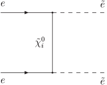
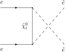
Figure 1: Feynman diagrams mediating the processes $e^{-}e^{-}\to\tilde{e}\,\tilde{e}$.

The dominant decay mode of the selectrons is $\tilde{e}\to e^{-}\tilde{\chi}_{1}^{0}$, leading to a final state with two electrons plus missing energy and momentum. The observation of this signal at sizeable rates is a clear indication of selectron pair production, although in principle it could also originate from other new physics processes. In this decay channel, the masses of the selectrons cannot be directly reconstructed, due to the presence of two unobservable neutralinos in the final state. However, the selectron masses can be precisely determined, for instance with a measurement of the total cross section at energies near threshold [10, 11]. In the continuum, the study of the electron energy spectrum shows that the produced particles are scalars, and the selectron masses can be extracted from the end points of this distribution [13]. Furthermore, it is possible to construct the minimum kinematically allowed selectron mass [14], whose distribution peaks at the actual selectron masses and hence yields another measurement of these quantities. The coincidence of all these measurements provides evidence for selectron pair production, and disfavours the interpretation of the $e^{-}e^{-}$ signal as originated by other new physics process.

With the same purpose, in this paper we consider a different decay channel which offers the advantage that the 4-momenta of all final state particles can be determined, and thus the selectron masses can be directly reconstructed event by event. This can be achieved restricting ourselves to $\tilde{e}_{L}\tilde{e}_{L}$ and $\tilde{e}_{R}\tilde{e}_{R}$ production, and selecting the channel where one of the selectrons decays to $e^{-}\tilde{\chi}_{1}^{0}$ and the other selectron decays via $\tilde{e}\to e^{-}\tilde{\chi}_{2}^{0}\to e^{-}\tilde{\chi}_{1}^{0}f\!\bar{f}$, with $f\!\bar{f}$ a $\mu^{-}\mu^{+}$ or $q\bar{q}$ pair. Although the latter is a relatively rare decay mode, if the selectrons are light enough to be produced at TESLA, the high luminosity available will allow us to obtain an observable signal in most cases. Using this channel alone, the direct reconstruction of the masses and the analysis of the two electron energy spectra (one resulting from $\tilde{e}\to e^{-}\tilde{\chi}_{1}^{0}$ and the other from $\tilde{e}\to e^{-}\tilde{\chi}_{2}^{0}$) provides clear evidence for selectron pair production. Since the reconstruction method introduced here allows the determination of the momenta of all final state particles, it can also be used for further studies of the angular distributions in the production and decay of the selectrons. In particular, it provides an independent direct verification that the selectrons are scalar particles. This analysis will be presented elsewhere [15].

This paper is organised as follows: In Section 2 we discuss the production and subsequent decay of selectron pairs in $e^{-}e^{-}$ collisions, and how these processes are generated. In Section 3 we briefly describe the model, outlining some important features, and we select two illustrative scenarios for $\mu^{+}\mu^{-}$ and $q\bar{q}$ final states. In Section 4 we describe how the reconstruction of the selectron masses is achieved and we present our results. Section 5 is devoted to our conclusions. In Appendix A we collect the mass matrices and Lagrangian terms which are relevant for our work. The benefits of beam polarisation for these processes are displayed in Appendix B.

2 Production and decay of selectron pairs in $\boldsymbol{e^{-}e^{-}}$ scattering

The reconstruction of the selectron masses is only possible for the production of two identical selectrons, $e^{-}e^{-}\to\tilde{e}_{L}\tilde{e}_{L},\tilde{e}_{R}\tilde{e}_{R}$ (this will be justified in the detailed discussion of Section 4). For these processes we choose the decay channels with one selectron decaying via $\tilde{e}\to e^{-}\tilde{\chi}_{1}^{0}$ and the other $\tilde{e}\to e^{-}\tilde{\chi}_{2}^{0}\to e^{-}\tilde{\chi}_{1}^{0}f\!\bar{f}$. In addition, we consider mixed selectron production $e^{-}e^{-}\to\tilde{e}_{R}\tilde{e}_{L}$, with $\tilde{e}_{R}\to e^{-}\tilde{\chi}_{1}^{0}$, $\tilde{e}_{L}\to e^{-}\tilde{\chi}_{2}^{0}\to e^{-}\tilde{\chi}_{1}^{0}f\!\bar{f}$, since this is the main background to the two processes of interest. Each of the processes

$$e^{-}e^{-}\to\tilde{e}_{L}\tilde{e}_{L}\to e^{-}\tilde{\chi}_{1}^{0}e^{-}\tilde{\chi}_{2}^{0}\to e^{-}\tilde{\chi}_{1}^{0}e^{-}\tilde{\chi}_{1}^{0}f\!\bar{f}$$

$$e^{-}e^{-}\to\tilde{e}_{R}\tilde{e}_{R}\to e^{-}\tilde{\chi}_{1}^{0}e^{-}\tilde{\chi}_{2}^{0}\to e^{-}\tilde{\chi}_{1}^{0}e^{-}\tilde{\chi}_{1}^{0}f\!\bar{f}$$

$$e^{-}e^{-}\to\tilde{e}_{R}\tilde{e}_{L}\to e^{-}\tilde{\chi}_{1}^{0}e^{-}\tilde{\chi}_{2}^{0}\to e^{-}\tilde{\chi}_{1}^{0}e^{-}\tilde{\chi}_{1}^{0}f\!\bar{f}$$ (1)

is mediated by 56 Feynman diagrams, depicted in Figs. 2 and 3. Although for clarity the diagrams for the decay of $\tilde{\chi}^{0}_{2}$ are shown separately, in our computations all the diagrams are summed coherently. We only consider final states with $f\!\bar{f}=\mu^{+}\mu^{-},q\bar{q}$, and in the case of $q\bar{q}$ we sum $u\bar{u}$, $d\bar{d}$, $s\bar{s}$, $c\bar{c}$ and $b\bar{b}$ production, without flavour tagging. Concerning the remaining channels, in $\tilde{\chi}_{2}^{0}\to\tilde{\chi}_{1}^{0}e^{+}e^{-}$ the multiplicity of electrons in the final state makes it difficult to identify the electron resulting from the decay of the $\tilde{\chi}_{2}^{0}$. In $\tilde{\chi}_{2}^{0}\to\tilde{\chi}_{1}^{0}\nu\bar{\nu}$ the presence of four undetected particles in the final state yields too many unmeasured momenta to allow their kinematical determination. The same happens in $\tilde{\chi}_{2}^{0}\to\tilde{\chi}_{1}^{0}\tau^{+}\tau^{-}$, because each of the $\tau$ leptons decays producing one or two neutrinos that escape detection.

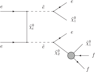
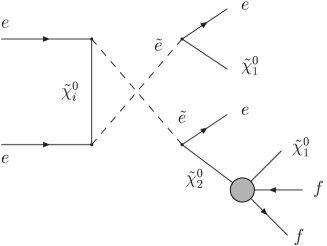
Figure 2: Feynman diagrams for the processes in Eqs. (1). The 4 neutralinos are exchanged in the $t$ channel, and the shaded circles stand for the 7 sub-diagrams mediating the decay of $\tilde{\chi}_{2}^{0}$, separately shown in Fig. 3.

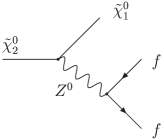
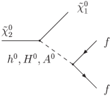
(a)		(b)
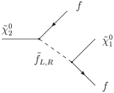
(c)		(d)

Figure 3: Feynman diagrams for the decay of $\tilde{\chi}^{0}_{2}$, mediated by $Z$ bosons (a), neutral Higgs bosons (b), and left-and right-handed scalar fermions (c and d).

Compared with $\tilde{e}_{R}\tilde{e}_{L}$ production, the other SUSY and SM backgrounds are less important. For instance, the process $e^{-}e^{-}\to\tilde{e}_{R}\tilde{e}_{R}f\!\bar{f}$, with both selectrons decaying to $e^{-}\tilde{\chi}_{1}^{0}$, has a smaller cross section, since it has the same number of vertices as $\tilde{e}_{R}\tilde{e}_{L}$ (both amplitudes are proportional to $g^{6}$) and does not have the enhancement of the $\tilde{\chi}_{2}^{0}$ near its mass shell. The main SM background is $e^{-}e^{-}\to e^{-}e^{-}\nu\bar{\nu}f\!\bar{f}$, including resonant $e^{-}e^{-}\to W^{-}e^{-}\nu f\!\bar{f}$ and $e^{-}e^{-}\to e^{-}e^{-}Zf\!\bar{f}$ production. This process has a small cross section and is separable from the $\tilde{e}_{L}\tilde{e}_{L}$, $\tilde{e}_{R}\tilde{e}_{R}$ signals, which have larger values for the missing energy and momentum. One might also consider the process $e^{-}e^{-}\to W^{-}W^{-}f\!\bar{f}$ mediated by heavy Majorana neutrinos. The cross section for the latter is very constrained by present limits on neutrinoless double beta decay [16], and this process could also be separated from selectron pair production, using the missing energy and momentum.

We calculate the full matrix elements for the resonant processes in Eqs. (1) with HELAS [17], using the Feynman rules for Majorana fermions given in Ref. [18]. The inclusion of next-to-leading order corrections is not necessary in this work, since it only increases slightly the cross sections [19]. We assume a centre of mass (CM) energy $E_{\mathrm{CM}}=2E=500$ GeV for the $e^{-}e^{-}$ collisions, and an integrated luminosity of 100 fb^-1. In order to take into account the effect of initial state radiation (ISR) on the effective beam energies, we convolute the differential cross section evaluated for fractions $x_{1}$, $x_{2}$ of the beam energies with “structure functions” $D_{\mathrm{ISR}}(x_{1})$ and $D_{\mathrm{ISR}}(x_{2})$, namely

$$d\sigma=\int_{0}^{1}d\sigma(x_{1}E,x_{2}E)D_{\mathrm{ISR}}(x_{1})D_{\mathrm{ISR}}(x_{2})dx_{1}dx_{2}\;.$$ (2)

The explicit expression for $D_{\mathrm{ISR}}$ used is [20]

$$D_{\mathrm{ISR}}(x) = \frac{\eta}{2}(1-x)^{\frac{\eta}{2}-1}\frac{e^{\frac{\eta}{2}\left(\frac{3}{4}-\gamma\right)}}{\Gamma\left(1+\frac{\eta}{2}\right)}$$ (3)

$$\times\left[\frac{1}{2}(1+x^{2})-\frac{\eta}{8}\left(\frac{1}{2}(1+3x^{2})\log x-(1-x)^{2}\right)\right]\;,$$

where

$$\eta(s)=-6\log\left[1-\frac{\alpha_{0}}{3\pi}\log\frac{s}{m_{e}^{2}}\right]\;,$$ (4)

$\gamma$ is the Euler constant, $\alpha_{0}=1/137$ the fine structure constant, $s=E_{\mathrm{CM}}^{2}$ and $m_{e}$ the electron mass. The effect of beamstrahlung is taken into account in a similar way using the “structure function” [21]

$$D_{\mathrm{BS}}(x)=e^{-N}\left[\delta(x-1)+\frac{e^{-\kappa(1-x)/x}}{x(1-x)}h(y)\right]\;,$$ (5)

where [22]

$$h(y)=\sum_{n=1}^{\infty}\frac{y^{n}}{n!\,\Gamma(n/3)}\;,$$ (6)

with $y=N[\kappa\,(1-x)/x]^{1/3}$. For large $y$, $h(y)$ has the asymptotic expansion

$$h(y)=\left(\frac{3z}{8\pi}\right)^{\frac{1}{2}}e^{4z}\left[1-\frac{35}{288\,z}-\frac{1295}{16588\,z^{2}}+\cdots\right]\;,$$ (7)

with $z=(y/3)^{3/4}$. We take $N=0.555$, $\kappa=0.0693$ [21] for our evaluations.

In order to simulate the calorimeter and tracking resolution, we perform a Gaussian smearing of the energies of electrons ($e$), jets ($j$) and muons ($\mu$) using the specifications in the TESLA Technical Design Report [23]

$$\frac{\Delta E^{e}}{E^{e}}=\frac{10\%}{\sqrt{E^{e}}}\oplus 1\%\;,\quad\frac{\Delta E^{j}}{E^{j}}=\frac{50\%}{\sqrt{E^{j}}}\oplus 4\%\;,\quad\frac{\Delta E^{\mu}}{E^{\mu}}=0.02\%\,E^{\mu}\;,$$ (8)

where the energies are in GeV and the two terms are added in quadrature. We apply “detector” cuts on transverse momenta, $p_{T}\geq 10$ GeV, and pseudorapidities $|\eta|\leq 2.5$, the latter corresponding to polar angles $10^{\circ}\leq\theta\leq 170^{\circ}$. We also reject events in which the leptons and/or jets are not isolated, requiring that the distances in $(\eta,\theta)$ space $\Delta R=\sqrt{\Delta\eta^{2}+\Delta\theta^{2}}$ satisfy $\Delta R\geq 0.4$. We do not require specific trigger conditions, and we assume that the presence of charged leptons with high transverse momentum will suffice. Finally, for the Monte Carlo integration in 8-body phase space we use RAMBO [24].

3 Overview of the model and selection of scenarios

The aim of the present work is to demostrate that the selectron masses can be successfully reconstructed with the method here proposed. It is nevertheless important to show that this can be done in realistic scenarios. In this section, we outline the main features of the model, and investigate the behaviour of the selectron production cross sections and decay rates as a function of the free parameters of the model.

In our analysis we consider the minimal supersymmetric standard model (MSSM), where a minimal number of fields is introduced and $R$-parity is conserved. For simplicity, we assume an underlying minimal supergravity (mSUGRA) [25] framework. At the grand unification scale, $M_{GUT}\simeq 2\times 10^{16}$ GeV, relations of universality among the several soft breaking terms allow the model to be described by five independent parameters: the common soft scalar mass ($m_{0}$), the unified gaugino mass ($m_{1/2}$), the universal trilinear coupling ($A_{0}$), the ratio of the two neutral Higgs vacuum expectation values ($\tan\beta=v_{2}/v_{1}$) and the sign of the bilinear Higgs term, $\operatorname{sign}(\mu)$. In our work we do not address supersymmetric CP violation, thus we assume that $m_{1/2}$ and $A_{0}$ are real. The low-energy Lagrangian is derived by means of the renormalisation group equations, which are numerically solved to the two-loop order using SPheno [26]. In addition, SPheno is used to obtain the masses and mixings of SUSY particles, as well as some decay widths. The mass matrices for sfermions and neutralinos and the required interaction terms are presented in Appendix A.

It is important to clarify here some issues, which are relevant for the subsequent discussion of selectron production and decay. The first concerns flavour and chirality mixing in the slepton sector. For the case of the first two generations, the $LR$ term in the slepton mass matrix (Eq. (A.3)) is significantly suppressed by the electron and muon Yukawa couplings. The smallness of $LR$ mixing for selectrons and smuons is fairly insensitive to the particular value of $A_{0}$, and for simplicity we choose $A_{0}=0$ in our numerical analysis. This typically translates into $\theta_{\tilde{e}}\sim\mathcal{O}(10^{-4})$ and $\theta_{\tilde{\mu}}\sim\mathcal{O}(10^{-2})$ (cf. Eq. (A.6)), so that $\tilde{e}_{L}\tilde{e}_{R}$ and $\tilde{\mu}_{L}\tilde{\mu}_{R}$ mixing can indeed be neglected. Therefore, for the first two generations the mass eigenstates are the chiral $(\tilde{e},\tilde{\mu})_{L}$, $(\tilde{e},\tilde{\mu})_{R}$ states. Moreover, leptonic interactions are assumed to be flavour-conserving, so only selectrons are produced in $e^{-}e^{-}$ collisions.

As afore mentioned, we assume that the lightest neutralino is the LSP. Depending on the underlying model, the $\tilde{\chi}^{0}_{1}$ can be gaugino- or higgsino-like, or a balanced admixture of the latter interaction eigenstates. Here we shall only consider cases where $\tilde{\chi}^{0}_{1}$ is gaugino-like and, more specifically, dominated by the bino component, a situation common to a vast region of the mSUGRA parameter space. In our case, the second neutralino, $\tilde{\chi}^{0}_{2}$, is dominated by the wino component, and thus its coupling to the right-handed selectron $\tilde{e}_{R}$ is very small. This fact has a significant impact in our analysis, since in this situation the $\tilde{e}_{R}$ mainly decays to $e^{-}\,\tilde{\chi}^{0}_{1}$, even when the $e^{-}\,\tilde{\chi}^{0}_{2}$ channel is kinematically allowed, so that the $\tilde{e}_{R}\tilde{e}_{R}$ process in Eq. (1) has a very small cross section. We emphasise that the reconstruction method proposed in this paper is not sensitive to the nature of the lightest neutralinos. However, the cross sections of the processes studied will be significantly affected, given that the relevant $\tilde{\chi}^{0}_{1}$-fermion-sfermion couplings are suppressed if the lightest neutralinos are higgsino-like.

The numerical studies presented in this section do not aim to be a complete scan of the available parameter space, but rather an illustrative analysis of the impact of the variation of the mSUGRA parameters on the selectron production and decay cross sections. In the following, we will simultaneously try to satisfy the direct and indirect bounds on the masses of the particles [27] and still obtain an adequate spectrum for sleptons and neutralinos, so that the processes in Eq. (1) can be observed at TESLA with a CM energy of 500 GeV.

We begin the selection of the scenarios by considering the dependence of the studied signals on $m_{0}$. This is shown in Fig. 4, for $\tilde{e}_{L}\tilde{e}_{L}$, $\tilde{e}_{R}\tilde{e}_{L}$ and $\tilde{e}_{R}\tilde{e}_{R}$ production (full, dashed and dot-dashed lines) and for the $\mu^{+}\mu^{-}$ and $q\bar{q}$ channels (black and grey lines, respectively). We have taken $m_{1/2}=220\ {\mathrm{GeV}}$, $\tan\beta=10$, and $\mu>0$. The shaded area on the left corresponds to values of $m_{0}$ excluded by the current experimental bounds on $m_{\tilde{e}_{R}}$ [27]. In addition, the end points of the curves marked with a circle correspond to the values of $m_{0}$ below which the lightest neutralino is not the LSP. In this section we consider unpolarised beams; the effect of longitudinal polarisation is discussed in Appendix B.

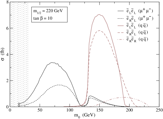
Figure 4: Cross sections (in fb) for $e^{-}e^{-}\to\tilde{e}\tilde{e}\to e^{-}\tilde{\chi}_{1}^{0}e^{-}\tilde{\chi}_{2}^{0}\to e^{-}\tilde{\chi}_{1}^{0}e^{-}\tilde{\chi}_{1}^{0}f\!\bar{f}$ (with unpolarised beams) as a function of $m_{0}$, for $m_{1/2}=220$ GeV and $\tan\beta=10$.

From this plot we notice that only for $m_{0}\geq 140$ GeV the $\tilde{e}_{R}$ is heavy enough to decay into the second neutralino. The shape of the curves reflects the strong dependence on $m_{0}$ of the production cross sections and branching ratios for $\tilde{e}_{L}\to\tilde{e}^{-}\chi_{2}^{0}$ and $\tilde{\chi}_{2}^{0}\to\tilde{\chi}_{1}^{0}f\!\bar{f}$. In the latter case, there are several competing Feynman diagrams [28, 29], mediated by the $Z$ boson and sfermions, that contribute to the decay of the $\tilde{\chi}_{2}^{0}$ (the contribution of the diagrams with a Higgs boson is small for this value of $\tan\beta$). Three different regimes can be distinguished:

• For $m_{0}\lesssim 120$ GeV, the second neutralino decays predominantly to charged leptons, $\tilde{\chi}_{2}^{0}\to\tilde{\chi}_{1}^{0}l^{+}l^{-}$. The decay amplitudes are dominated by diagrams (c) and (d) in Fig. 3, with the exchange of on-shell right-handed sleptons, in particular the decay $\tilde{\chi}_{2}^{0}\to\tilde{\chi}_{1}^{0}\mu^{+}\mu^{-}$ is dominated by $\tilde{\mu}_{R}$ exchange. The contribution of diagram (a) with an on-shell $Z$ boson is less important, due to the smallness of the $Z\tilde{\chi}_{2}^{0}\tilde{\chi}_{1}^{0}$ coupling. In this region of the parameter space, the decays to $\tilde{\chi}_{1}^{0}q\bar{q}$ are very suppressed, not only because of the small coupling of the $Z$ boson to $\tilde{\chi}_{1}^{0}$ and $\tilde{\chi}_{2}^{0}$, but also due to the heavy squark masses, $m_{\tilde{q}}\gtrsim 400$ GeV.

• For $m_{0}\sim 130$ GeV, the $\tilde{e}_{R}$ and $\tilde{\mu}_{R}$ are heavier than the $\tilde{\chi}_{2}^{0}$, while the $\tilde{\tau}_{R}$ is lighter. Then, the $\tilde{\chi}_{2}^{0}$ decays almost exclusively to $\tilde{\chi}_{1}^{0}\tau^{+}\tau^{-}$, mediated by an on-shell $\tilde{\tau}_{R}$, diagrams (c) and (d) in Fig. 3. (As remarked in Section 2, in the $\tau^{+}\tau^{-}$ channel the selectron masses cannot be reconstructed, and thus we do not consider these final states in the plots presented throughout this section.)

• For $m_{0}\gtrsim 140$ GeV, the right-handed sleptons (including $\tilde{\tau}_{R}$) are heavier than $\tilde{\chi}_{2}^{0}$, and the $Z$-exchange diagram in Fig. 3 dominates, yielding a large branching ratio for $\tilde{\chi}_{2}^{0}\to\tilde{\chi}_{1}^{0}q\bar{q}$.

For $m_{0}\gtrsim 200$ GeV, the production of $\tilde{e}_{L}\tilde{e}_{L}$ and $\tilde{e}_{L}\tilde{e}_{R}$ is not possible with a CM energy of 500 GeV, and only $\tilde{e}_{R}\tilde{e}_{R}$ pairs are produced. From inspection of Fig. 4 we select two values $m_{0}=80$ GeV and $m_{0}=160$ GeV, approximately in the centre of the first and third regions, that will serve to illustrate the reconstruction of the selectron masses for $\mu^{+}\mu^{-}$ and $q\bar{q}$ final states. The sets of parameters for these two mSUGRA scenarios are summarised in Table 1. Both of them are in agreement with the bounds arising from the $b\to s\gamma$ decay [27], and they are in the region of the $(m_{1/2},m_{0})$ plane favoured by $(g-2)_{\mu}$ at the $2\,\sigma$ level [30]. The resulting selectron and neutralino masses and widths, as well as the relevant branching ratios, are collected in Table 2 for each of these scenarios. In scenario 1 the $\tilde{e}_{R}$ is lighter than the $\tilde{\chi}_{2}^{0}$, and the decay $\tilde{e}_{R}\to e^{-}\tilde{\chi}_{2}^{0}$ is not possible. Hence, in this scenario we only consider the $\tilde{e}_{L}\tilde{e}_{L}$ signal.

Parameter		Scenario 1		Scenario 2
$m_{1/2}$		220		220
$m_{0}$		80		160
$A_{0}$		0		0
$\tan\beta$		10		10
$\mathrm{sign}\,\mu$		$+$		$+$

Table 1: Input parameters for the two mSUGRA scenarios to be considered in Section 4. The values of $m_{1/2}$, $m_{0}$ and $A_{0}$ are in GeV.

	Scenario 1		Scenario 2
$m_{\tilde{e}_{L}}$	181.0		227.4
$\Gamma_{\tilde{e}_{L}}$	0.25		0.85
$m_{\tilde{e}_{R}}$	123.0		185.0
$\Gamma_{\tilde{e}_{R}}$	0.17		0.58
$m_{\tilde{\chi}_{1}^{0}}$	84.0		84.3
$m_{\tilde{\chi}_{2}^{0}}$	155.8		156.4
$\Gamma_{\tilde{\chi}_{2}^{0}}$	0.023		$1.50\times 10^{-5}$
$m_{\tilde{\chi}_{3}^{0}}$	309.4		310.0
$\Gamma_{\tilde{\chi}_{3}^{0}}$	1.48		1.43
$m_{\tilde{\chi}_{4}^{0}}$	330.4		331.1
$\Gamma_{\tilde{\chi}_{4}^{0}}$	2.30		2.01
$\mathrm{Br}(\tilde{e}_{L}\to e^{-}\tilde{\chi}_{1}^{0})$	41.8 %		18.3 %
$\mathrm{Br}(\tilde{e}_{L}\to e^{-}\tilde{\chi}_{2}^{0})$	20.6 %		30.8 %
$\mathrm{Br}(\tilde{e}_{R}\to e^{-}\tilde{\chi}_{1}^{0})$	100 %		99.7 %
$\mathrm{Br}(\tilde{e}_{R}\to e^{-}\tilde{\chi}_{2}^{0})$	$\simeq 0$		0.3 %
$\mathrm{Br}(\tilde{\chi}_{2}^{0}\to\tilde{\chi}_{1}^{0}\mu^{+}\mu^{-})$	10.3 %		3.9 %
$\mathrm{Br}(\tilde{\chi}_{2}^{0}\to\tilde{\chi}_{1}^{0}q\bar{q})$	$\simeq 0$		69.2 %

Table 2: Some relevant quantities in the two mSUGRA scenarios considered in Section 4. The masses and widths are in GeV.

For completeness, we investigate the dependence of the cross sections on the remaining parameters. For scenario 1, and leaving all other parameters as in Table 1, we plot in Fig. 5 the cross sections for different values of $m_{1/2}$. The shaded area on the left corresponds to values of $m_{1/2}$ that yield a $\tilde{\chi}_{1}^{0}$ mass excluded by present limits [27]. Note that the depression occurring around $m_{1/2}=160$ GeV has the same origin as the one observed in Fig. 4, and corresponds to the dominance of the $\tau^{+}\tau^{-}$ decay channel. The decrease of the cross sections for large $m_{1/2}$ is caused by the reduction in the branching ratio for $\tilde{e}_{L}\to e^{-}\tilde{\chi}_{2}^{0}$ and is also a consequence of the smaller phase space available for selectron pair production. In fact, with $m_{0}=80$ GeV, the production of $\tilde{e}_{L}\tilde{e}_{L}$ pairs is only kinematically possible when $m_{1/2}\leq 340$ GeV.

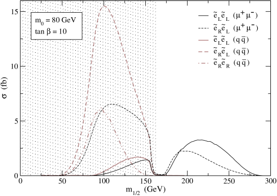
Figure 5: Cross sections (in fb) for $e^{-}e^{-}\to\tilde{e}\tilde{e}\to e^{-}\tilde{\chi}_{1}^{0}e^{-}\tilde{\chi}_{2}^{0}\to e^{-}\tilde{\chi}_{1}^{0}e^{-}\tilde{\chi}_{1}^{0}f\!\bar{f}$ (with unpolarised beams) as a function of $m_{1/2}$, for $m_{0}=80$ GeV and $\tan\beta=10$.

For scenario 2, we fix $m_{0}=160$ GeV, $\tan\beta=10$, $A_{0}=0$ (as in Table 1), and plot the cross sections for different values of $m_{1/2}$ (see Fig. 6). The shaded area on the left of this figure corresponds to values of $m_{1/2}$ for which $m_{\tilde{\chi}_{1}^{0}}$ is excluded [27]. The sudden decrease of the cross sections for $m_{1/2}\gtrsim 250$ GeV is caused by both the dominance of the $\tau^{+}\tau^{-}$ channel and the small phase space available for selectron pair production. For $m_{0}=160$ GeV, the production of $\tilde{e}_{L}\tilde{e}_{L}$ pairs is kinematically forbidden with $m_{1/2}\geq 270$ GeV. The production of $\tilde{e}_{R}\tilde{e}_{R}$ pairs is still allowed, but for $m_{1/2}\geq 260$ GeV the $\tilde{\chi}_{2}^{0}$ is heavier than the $\tilde{e}_{R}$ and the decay $\tilde{e}_{R}\to e^{-}\tilde{\chi}_{2}^{0}$ is not possible.

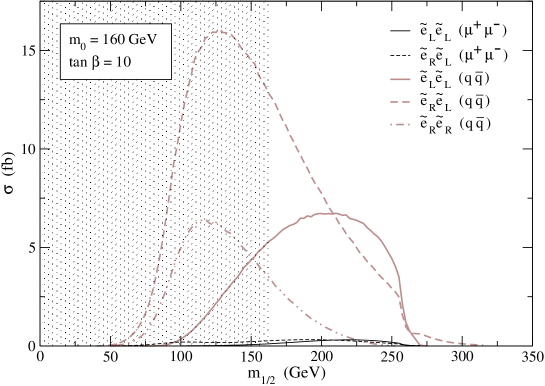
Figure 6: Cross sections (in fb) for $e^{-}e^{-}\to\tilde{e}\tilde{e}\to e^{-}\tilde{\chi}_{1}^{0}e^{-}\tilde{\chi}_{2}^{0}\to e^{-}\tilde{\chi}_{1}^{0}e^{-}\tilde{\chi}_{1}^{0}f\!\bar{f}$ (with unpolarised beams) as a function of $m_{1/2}$, for $m_{0}=160$ GeV and $\tan\beta=10$.

We also examine the dependence of the cross sections on $\tan\beta$ for scenarios 1 and 2. Fixing $m_{1/2}=220$ GeV, $m_{0}=80,160$ GeV, $A_{0}=0$ (as in Table 1), we plot in Figs. 7 and 8, respectively, the cross sections for different values of $\tan\beta$. In both figures the shaded areas on the left are excluded by the LEP bounds on the MSSM lightest Higgs mass, and in Fig. 7 the end points of the curves marked with a circle correspond to values of $\tan\beta$ for which the LSP is no longer $\tilde{\chi}_{1}^{0}$. In both cases the regions of parameter space for which the process $e^{-}e^{-}\to\tilde{e}_{L}\tilde{e}_{L}\to e^{-}\tilde{\chi}_{1}^{0}e^{-}\tilde{\chi}_{1}^{0}f\!\bar{f}$ is observable range up to $\tan\beta\simeq 22$.

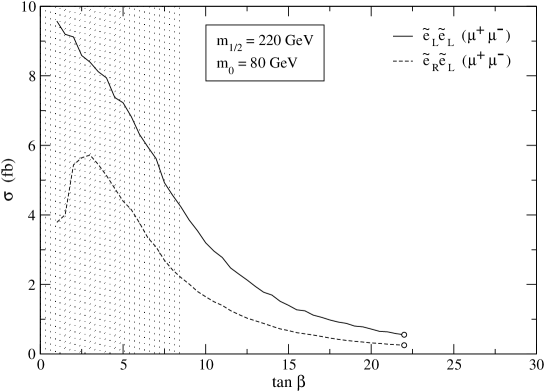
Figure 7: Cross sections (in fb) for $e^{-}e^{-}\to\tilde{e}\tilde{e}\to e^{-}\tilde{\chi}_{1}^{0}e^{-}\tilde{\chi}_{2}^{0}\to e^{-}\tilde{\chi}_{1}^{0}e^{-}\tilde{\chi}_{1}^{0}f\!\bar{f}$ (with unpolarised beams) as a function of $\tan\beta$, for $m_{1/2}=220$ GeV and $m_{0}=80$ GeV.

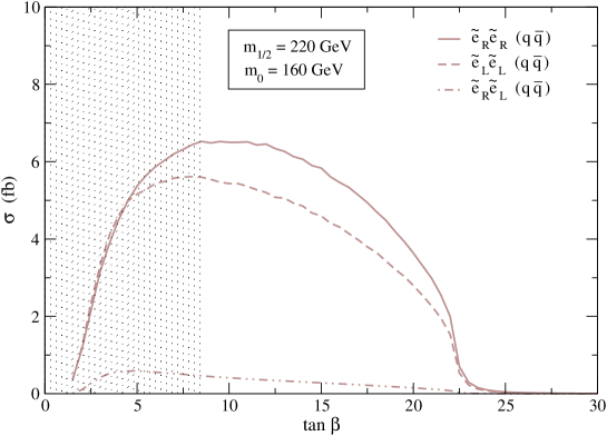
Figure 8: Cross sections (in fb) for $e^{-}e^{-}\to\tilde{e}\tilde{e}\to e^{-}\tilde{\chi}_{1}^{0}e^{-}\tilde{\chi}_{2}^{0}\to e^{-}\tilde{\chi}_{1}^{0}e^{-}\tilde{\chi}_{1}^{0}f\!\bar{f}$ (with unpolarised beams) as a function of $\tan\beta$, for $m_{1/2}=220$ GeV and $m_{0}=160$ GeV.

The study of Figs. 4–8 reveals that for most regions of mSUGRA parameter space where $\tilde{e}_{L}\tilde{e}_{L}$ production is kinematically accesible, either the $\mu^{+}\mu^{-}$ or the $q\bar{q}$ decay channels have observable cross sections. The only exceptions are narrow intervals in $m_{0}$ and $m_{1/2}$, and also large $\tan\beta$ values, where the $\tau^{+}\tau^{-}$ channel completely dominates the $\tilde{\chi}_{2}^{0}$ decays. On the other hand, the cross section for $e^{-}e^{-}\to\tilde{e}_{R}\tilde{e}_{R}\to e^{-}\tilde{\chi}_{1}^{0}e^{-}\tilde{\chi}_{2}^{0}\to e^{-}\tilde{\chi}_{1}^{0}e^{-}\tilde{\chi}_{1}^{0}f\!\bar{f}$ is always small, as a consequence of the small branching ratio for $\tilde{e}_{R}\to e^{-}\tilde{\chi}_{2}^{0}$ (in addition, this decay mode is not possible when $m_{\tilde{e}_{R}}\lesssim m_{\tilde{\chi}_{2}^{0}}$). Finally, we remark that, as shown in Figs. 4–6, for larger values of $m_{1/2}$ and/or $m_{0}$ selectron pair production and, in general, the production of supersymmetric particles, is not kinematically allowed at the assumed CM energy of 500 GeV, and a higher energy collider (or the TESLA upgrade) would be required for studies involving a heavier SUSY spectrum.

4 Reconstruction of the selectron masses

To reconstruct the selectron masses we use as input the 4-momenta of the detected particles (the two electrons and the $f\!\bar{f}$ pair), the CM energy and the $\tilde{\chi}_{1}^{0}$ and $\tilde{\chi}_{2}^{0}$ masses, which we assume known from other experiments [6, 13]. Remarkably, the values of both selectron masses are not needed anywhere. Let us first fix our notation by labelling the two electrons in the final state as “electron $a$” and “electron $b$” (either choice is equivalent) and their momenta as $p_{a}=(E_{a},\vec{p}_{a})$ and $p_{b}=(E_{b},\vec{p}_{b})$. The selectrons to which they correspond are then called “selectron $a$” and “selectron $b$”, and the $\tilde{\chi}_{1}^{0}$ resulting from the decay of the latter are also labelled as “$a$” and “$b$”, with momenta $q_{a}=(E_{a}^{\prime},\vec{q}_{a})$ and $q_{b}=(E_{b}^{\prime},\vec{q}_{b})$, respectively. The momentum of the $f\!\bar{f}$ pair is denoted as $p_{f\!\bar{f}}=(E_{f\!\bar{f}},\vec{p}_{f\!\bar{f}})$.

In general, it is necessary to have as many kinematical relations as unknown variables in order to determine the momenta of the undetected particles. In our case, there are 8 unknowns (the 4 components of $q_{a}$ and $q_{b}$) and 8 constraints. From energy and momentum conservation and the fact that the two $\tilde{\chi}_{1}^{0}$ are on shell, we have

$$E_{a}^{\prime}+E_{b}^{\prime} = E_{\mathrm{CM}}-(E_{a}+E_{b}+E_{f\!\bar{f}})\;,$$

$$\vec{q}_{a}+\vec{q}_{b} = \vec{p}\!\!\!\!\!\not\,\,\,\,\;,$$

$$q_{a}^{2} = m_{\tilde{\chi}_{1}^{0}}^{2}\;,$$

$$q_{b}^{2} = m_{\tilde{\chi}_{1}^{0}}^{2}\;,$$ (9)

with $\vec{p}\!\!\!\!\!\not\,\,\,\,$ the missing momentum. Another equation is obtained from the decay of the intermediate $\tilde{\chi}_{2}^{0}$. Since we do not know a priori which selectron decays to $\tilde{\chi}_{2}^{0}$, we must consider both possibilities. If we assume that it is the selectron “$a$”, we have

$$(q_{a}+p_{f\!\bar{f}})^{2}=m_{\tilde{\chi}_{2}^{0}}^{2}\hskip 133.72786pt\mbox{[case (a)]}\;,$$ (10)

or, assuming it is the selectron “$b$”,

$$(q_{b}+p_{f\!\bar{f}})^{2}=m_{\tilde{\chi}_{2}^{0}}^{2}\hskip 133.72786pt\mbox{[case (b)]}\;.$$ (11)

In order to set the last kinematical constraint, we make the hypothesis that in the $e^{-}e^{-}$ scattering two particles of equal mass are produced. This implies that in one case we have

$$E_{a}+E_{a}^{\prime}+E_{f\!\bar{f}}=E_{b}+E_{b}^{\prime}\hskip 85.35826pt\mbox{[case (a)]}$$ (12)

while in the other

$$E_{a}+E_{a}^{\prime}=E_{b}+E_{b}^{\prime}+E_{f\!\bar{f}}\hskip 85.35826pt\mbox{[case (b)]}\;.$$ (13)

It is worthwhile remarking that ISR, beamstrahlung, particle width effects and detector resolution degrade the determination of the $\tilde{\chi}_{1}^{0}$ momenta. The ISR and beamstrahlung modify the effective beam energies, and therefore the first two of Eqs. (9) do not hold exactly. The finite detector resolution also implies that Eqs. (9–13) are only approximate. Moreover, the off-shellness of the selectrons and of the $\tilde{\chi}_{2}^{0}$ have a non-negligible influence on Eqs. (10–13). As a result of all these effects, in some cases the solutions of these equations are imaginary, even when the $\tilde{\chi}_{2}^{0}$ is “correctly” assigned to a selectron. In order to find a real solution in any circumstance, we force the discriminants of the second degree equations involved to be non-negative.

Each set of equations – Eqs. (9,10,12) and Eqs. (9,11,13) – yields two solutions for $q_{a}$ and $q_{b}$. Among these four solutions, we have to select one, which in turn gives a value for the reconstructed mass. To do so, we observe the following criteria:

1. We first eliminate the unphysical solutions yielding negative reconstructed selectron masses $m_{\tilde{e}}^{\mathrm{rec}}$.

2. We then discard the solutions in which the reconstructed mass of the $\tilde{\chi}_{2}^{0}$, $m_{\tilde{\chi}_{2}^{0}}^{\mathrm{rec}}$, is too different from the real value: for the $\mu^{+}\mu^{-}$ channel we require $|m_{\tilde{\chi}_{2}^{0}}^{\mathrm{rec}}-m_{\tilde{\chi}_{2}^{0}}|\leq 5$ GeV, and for the $q\bar{q}$ channel $|m_{\tilde{\chi}_{2}^{0}}^{\mathrm{rec}}-m_{\tilde{\chi}_{2}^{0}}|\leq 10$ GeV.

3. Among the remaining solutions, we take the one giving the smallest value of $m_{\tilde{e}}^{\mathrm{rec}}$. This choice provides the “correct” solution in most cases. If no solution is left after (II), the event is discarded.

The above procedure determines the momenta of the two unobserved $\tilde{\chi}_{1}^{0}$, identifying which selectron has decayed to $\tilde{\chi}_{2}^{0}$ as well, allowing to reconstruct the selectron masses. The reconstruction also allows to distinguish between the electrons resulting from $\tilde{e}\to e^{-}\tilde{\chi}_{1}^{0}$, and $\tilde{e}\to e^{-}\tilde{\chi}_{2}^{0}$. Let us define $E_{1}$ and $E_{2}$ as the energies of the electrons produced in the decays $\tilde{e}\to e^{-}\tilde{\chi}_{1}^{0}$, and $\tilde{e}\to e^{-}\tilde{\chi}_{2}^{0}$, respectively. In the selectron rest frame, the electron energy is fixed by the kinematics of the 2-body decay, and since the selectrons are spinless particles, the decay is isotropic. Then, for $\tilde{e}_{L}\tilde{e}_{L}$, $\tilde{e}_{R}\tilde{e}_{R}$ production the energy distribution of the electrons in the CM frame is flat, with end points at [14, 32]

$$E_{i}^{\mathrm{max}} = \frac{\sqrt{s}}{4}\left(1-\frac{m_{\tilde{\chi}_{i}^{0}}^{2}}{m_{\tilde{e}_{L,R}}^{2}}\right)(1+\beta)\;,$$

$$E_{i}^{\mathrm{min}} = \frac{\sqrt{s}}{4}\left(1-\frac{m_{\tilde{\chi}_{i}^{0}}^{2}}{m_{\tilde{e}_{L,R}}^{2}}\right)(1-\beta)\;,$$ (14)

where $\beta=\sqrt{1-4m_{\tilde{e}_{L,R}}^{2}/s}$. For mixed selectron production the electron energy spectra are flat as well, but the expressions of the end points are more involved. The results for the reconstruction are illustrated for scenarios 1 and 2.

4.1 Scenario 1

As seen from Fig. 9, in scenario 1 the reconstruction of the $\tilde{e}_{L}$ mass is quite effective, and a sharp peak at the true value $m_{\tilde{e}_{L}}=181$ GeV (as given in Table 2) is obtained. On the other hand, the distribution of the $\tilde{e}_{R}\tilde{e}_{L}$ events is rather flat. We notice that the criteria (I,II) in the reconstruction procedure operate as an efficient kinematical cut, suppressing the unwanted $\tilde{e}_{R}\tilde{e}_{L}$ production, while for $\tilde{e}_{L}\tilde{e}_{L}$ the effect is much smaller (cf. Table 3). Assuming an integrated luminosity of 100 fb^-1, the number of events collected in the detector is sufficiently large to allow the observation of a positive signal, with a mass distribution concentrated at $m_{\tilde{e}_{L}}=181$ GeV. The use of negative beam polarisation $P_{1}=P_{2}=-0.8$ improves these results, increasing the $\tilde{e}_{L}\tilde{e}_{L}$ cross section by a factor of 3.24 and reducing the $\tilde{e}_{R}\tilde{e}_{L}$ cross section by a factor of 0.36 (see Table 3 and Appendix B).

Figure 9: Reconstructed selectron mass in scenario 1, for unpolarised beams.

		$P_{00}$			$P_{--}$
		before	after		before	after
$\tilde{e}_{L}\tilde{e}_{L}$		3.25	2.88		10.52	9.32
$\tilde{e}_{R}\tilde{e}_{L}$		1.66	0.47		0.60	0.17

Table 3: Cross sections (in fb) for selectron pair production in scenario 1. We quote results before and after reconstruction, for unpolarised beams ($P_{00}$) and for $P_{1}=P_{2}=-0.8$ ($P_{--}$).

The particles observed in the kinematical distribution in Fig. 9 are scalars, as can be easily deduced for instance from the angular distributions for the production and the decay [15]. The same can also be concluded from the analysis of the electron energy spectra, which also provides additional independent determinations of their mass. From Eqs. (14), the expected end points of the distributions are $E_{1}^{\mathrm{min}}=30$ GeV, $E_{1}^{\mathrm{max}}=166$ GeV and $E_{2}^{\mathrm{min}}=10$ GeV, $E_{2}^{\mathrm{max}}=55$ GeV. The kinematical distributions of $E_{1}$ and $E_{2}$ are shown in Figs. 10 and 11, respectively. We have included the $\tilde{e}_{L}\tilde{e}_{L}$ signal, as well as the $\tilde{e}_{R}\tilde{e}_{L}$ background. The energy spectrum of the electrons is smeared by ISR, beamstrahlung, detector resolution and particle width effects. However, the end points can be clearly observed in both plots, further supporting the evidence for $\tilde{e}_{L}\tilde{e}_{L}$ production.

Figure 10: Kinematical distribution of $E_{1}$ in scenario 1, for unpolarised beams.

Figure 11: Kinematical distribution of $E_{2}$ in scenario 1, for unpolarised beams.

4.2 Scenario 2

In this scenario, the $\tilde{e}_{L}\tilde{e}_{L}$ events produce a peak at $m_{\tilde{e}_{L}}=227$ GeV, and the $\tilde{e}_{R}\tilde{e}_{R}$ events yield a tiny peak around $m_{\tilde{e}_{R}}=185$ GeV, as depicted in Fig. 12. Noticeably, the distribution of the $\tilde{e}_{R}\tilde{e}_{L}$ events concentrates around $215$ GeV. This behaviour is a result of the smaller ratio $(m_{\tilde{e}_{L}}-m_{\tilde{e}_{R}})/(m_{\tilde{e}_{L}}+m_{\tilde{e}_{R}})$: in this scenario, the hypothesis of two particles produced with equal mass, used for the reconstruction, becomes more accurate. For the same reason, in this case this background is less reduced by the criteria (I,II) than in scenario 1. We observe that the $\tilde{e}_{L}\tilde{e}_{L}$ peak is broader than in scenario 1, due to the larger $\tilde{e}_{L}$ width and the less precise measurement of the energy for jets. Additionally, the distribution is slightly concentrated on smaller $m_{\tilde{e}_{R}}$ values, as a consequence of the procedure used for the reconstruction.

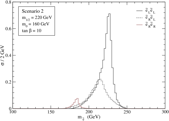
Figure 12: Reconstructed selectron masses in scenario 2, for unpolarised beams.

		$P_{00}$			$P_{--}$			$P_{++}$
		before	after		before	after		before	after
$\tilde{e}_{L}\tilde{e}_{L}$		6.52	5.71		21.14	18.50		0.26	0.23
$\tilde{e}_{R}\tilde{e}_{R}$		0.41	0.34		0.02	0.01		1.34	1.10
$\tilde{e}_{R}\tilde{e}_{L}$		5.41	2.63		1.95	0.95		1.95	0.95

Table 4: Cross sections (in fb) for selectron pair production in scenario 2. We quote results before and after reconstruction, for unpolarised beams ($P_{00}$), for $P_{1}=P_{2}=-0.8$ ($P_{--}$) and for $P_{1}=P_{2}=0.8$ ($P_{++}$).

The use of negative beam polarisation enhances the $\tilde{e}_{L}\tilde{e}_{L}$ signal and reduces the $\tilde{e}_{R}\tilde{e}_{L}$ background as in scenario 1, practically eliminating $\tilde{e}_{R}\tilde{e}_{R}$ production (see Table 4). Conversely, the use of positive beam polarisation $P_{1}=P_{2}=0.8$ enhances $\tilde{e}_{R}\tilde{e}_{R}$ by a factor of 3.24, suppressing $\tilde{e}_{L}\tilde{e}_{L}$ and $\tilde{e}_{R}\tilde{e}_{L}$ by factors of 0.04 and 0.36, respectively, and making the $\tilde{e}_{R}\tilde{e}_{R}$ peak clearly visible in this case, as shown in Appendix B.

The examination of the energy spectra in Figs. 13 and 14 confirms the evidence of $\tilde{e}_{L}\tilde{e}_{L}$ production. From Eqs. (14) we obtain for the decay $\tilde{e}_{L}\to e^{-}\tilde{\chi}_{1}^{0}$ the end points $E_{1}^{\mathrm{min}}=63$ GeV, $E_{1}^{\mathrm{max}}=153$ GeV, and for $\tilde{e}_{L}\to e^{-}\tilde{\chi}_{2}^{0}$ the limits $E_{2}^{\mathrm{min}}=38$ GeV, $E_{2}^{\mathrm{max}}=93$ GeV. In this scenario the $\tilde{e}_{R}\tilde{e}_{L}$ background is sizeable, and negative beam polarisation might be needed in order to clearly determine the end points of the electron energy distributions. (Note that the large distortion in the energy spectra for $\tilde{e}_{R}\tilde{e}_{L}$ is a result of the reconstruction process, which is devised for the $\tilde{e}_{L}\tilde{e}_{L}$ and $\tilde{e}_{R}\tilde{e}_{R}$ signals.) The electron energy distributions in $\tilde{e}_{R}\tilde{e}_{R}$ production display the end points at the expected energies $E_{1}^{\mathrm{min}}=32$ GeV, $E_{1}^{\mathrm{max}}=166$ GeV, $E_{2}^{\mathrm{min}}=12$ GeV and $E_{2}^{\mathrm{max}}=60$ GeV. For an integrated luminosity of 100 fb^-1, these end points may be hard to observe even with positive beam polarisation, because of the small cross section and the poor statistics for this process. However, for larger luminosities the end points could be observed more clearly (see Appendix B).

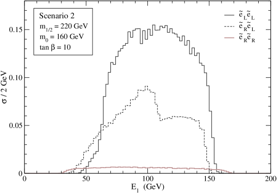
Figure 13: Kinematical distribution of $E_{1}$ in scenario 2, for unpolarised beams.

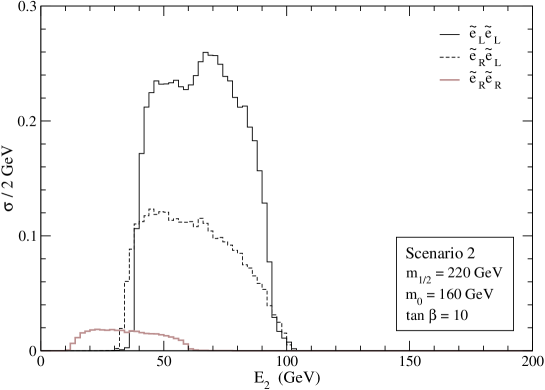
Figure 14: Kinematical distribution of $E_{2}$ in scenario 2, for unpolarised beams.

5 Conclusions

In this paper we have focused on the experimental test of the Majorana nature of the neutralinos, studying selectron pair production in $e^{-}e^{-}$ scattering. These processes can only take place if, as it is predicted in most SUSY models, the neutralinos are Majorana particles. Motivated by this issue, we have demonstrated that it is possible to reconstruct the selectron masses in the processes $e^{-}e^{-}\to\tilde{e}_{L}\tilde{e}_{L},\tilde{e}_{R}\tilde{e}_{R}$, using a relatively rare channel with one selectron decaying to $e^{-}\tilde{\chi}_{1}^{0}$ and the other one decaying via $\tilde{e}\to e^{-}\tilde{\chi}_{2}^{0}\to e^{-}\tilde{\chi}_{1}^{0}f\!\bar{f}$. The reconstruction can be done using as input the 4-momenta of the detected particles, the CM energy and the $\tilde{\chi}_{1}^{0}$ and $\tilde{\chi}_{2}^{0}$ masses, which are assumed to be known. In addition, the reconstruction procedure allows for a determination of all final state momenta, which in turn has other potential applications [15]. We have illustrated our results in two mSUGRA scenarios. In the first scenario we have considered the channel $f\!\bar{f}=\mu^{+}\mu^{-}$, and in the second one the channel $f\!\bar{f}=q\bar{q}$. In the calculations we have taken into account ISR, beamstrahlung and particle width effects, and we have performed a simple simulation of the energy resolution of the detector. We have included the main background from $\tilde{e}_{R}\tilde{e}_{L}$ production as well. We have shown that for the kinematically allowed processes the masses can be successfully reconstructed in both scenarios, yielding a clear peak in the case of $\tilde{e}_{L}\tilde{e}_{L}$ production and a smaller peak for $\tilde{e}_{R}\tilde{e}_{R}$ production. The examination of the electron energy spectra shows that the produced particles are scalars, making it obvious that the observed signal corresponds to selectron pair production. Additionally, the electron energy distributions display end points at the energies expected for $\tilde{e}_{L}\tilde{e}_{L}$ and $\tilde{e}_{R}\tilde{e}_{R}$ production in each of the cases analysed, providing independent determinations of the selectron masses and further supporting the evidence for selectron pair production. Obviously, the hypothesis of selectron pair production can also be confirmed by comparing the reconstructed masses with the selectron masses precisely measured in other processes [10, 11].

In $e^{-}e^{-}$ collisions, selectron pair production requires the exchange of a Majorana neutralino in the $t$ channel, but does not prove that all the neutralinos are Majorana particles. However, if the neutralino mixing matrix is precisely reconstructed in other experiments [33, 34, 35], the measurement of the $\tilde{e}_{L}\tilde{e}_{L}$ and $\tilde{e}_{R}\tilde{e}_{R}$ cross sections may allow us to identify the contributions of the different neutralino mass eigenstates. In mSUGRA scenarios as those here considered, where the two lightest neutralino mass eigenstates are gaugino-like, $\tilde{e}_{R}\tilde{e}_{R}$ production is mainly mediated by the exchange of $\tilde{\chi}_{1}^{0}$, with a smaller contribution from $\tilde{\chi}_{2}^{0}$, the opposite occurring for $\tilde{e}_{L}\tilde{e}_{L}$ production. Then, in these scenarios the measurement of one or both cross sections can prove the exchange of Majorana neutralinos $\tilde{\chi}_{1}^{0}$ and $\tilde{\chi}_{2}^{0}$ (the analogous can be done in more general scenarios where the reverse situation occurs, that is, when $\tilde{\chi}_{1}^{0}$ is dominated by the wino component and $\tilde{\chi}_{2}^{0}$ is bino-like). The contribution to the cross sections of the neutralinos with large higgsino-like components ($\tilde{\chi}_{3}^{0}$ and $\tilde{\chi}_{4}^{0}$ in our case) is expected to be smaller than the uncertainty in the measurement of the cross sections.

It is worth noting here that in addition to selectron pair production in $e^{-}e^{-}$ collisions, the processes $e^{+}e^{-}\to\tilde{\chi}_{1}^{0}\tilde{\chi}_{i}^{0}\to\tilde{\chi}_{1}^{0}\tilde{\chi}_{1}^{0}l^{+}l^{-}$, with $i=2,3,4$ and $l=e,\mu$, may also shed light on the Dirac or Majorana nature of the neutralinos [7, 8, 9]. The energy distributions of the final state charged leptons are sensitive to the Dirac or Majorana nature of the decaying neutralino $\tilde{\chi}_{i}^{0}$, allowing for the construction of lepton energy asymmetries, which vanish for a Majorana $\tilde{\chi}_{i}^{0}$ but may have a nonzero value if $\tilde{\chi}_{i}^{0}$ is a Dirac particle. Unfortunately, these processes suffer from severe backgrounds from slepton pair production $e^{+}e^{-}\to\tilde{l}\tilde{l}\to l^{+}l^{-}\tilde{\chi}_{i}^{0}\tilde{\chi}_{i}^{0}$, as well as chargino pair $e^{+}e^{-}\to\tilde{\chi}_{i}^{+}\tilde{\chi}_{j}^{-}\to l^{+}l^{-}\nu_{l}\bar{\nu}_{l}\tilde{\chi}_{i}^{0}\tilde{\chi}_{i}^{0}$ and $W^{+}W^{-}$ production. Moreover, for the case of $\tilde{\chi}_{1}^{0}\tilde{\chi}_{3}^{0}$ and $\tilde{\chi}_{1}^{0}\tilde{\chi}_{4}^{0}$ the production cross sections and decay branching ratios are in general small. If these difficulties can be overcome, these processes may give further evidence of the Majorana or Dirac nature of $\tilde{\chi}_{2}^{0}$, $\tilde{\chi}_{3}^{0}$ and $\tilde{\chi}_{4}^{0}$.

In this work we have taken as example the TESLA collider with a CM energy of 500 GeV, but the analysis presented can be applied to the proposed TESLA upgrade to 800 GeV and other future colliders with larger CM energies, like CLIC. In this case, with the larger energies and luminosities the processes studied will be relevant in a larger region of parameter space, which is not kinematically accesible at 500 GeV. Due to the $t$-channel nature of these processes, their cross sections remain sizeable at TeV energies and hence allow us to investigate the Majorana nature of the neutralinos in the case of a heavier SUSY spectrum too. Finally, let us remark the importance of the reconstruction of the selectron masses on its own. This novel reconstruction technique can also be used, for instance, in selectron and smuon pair production in $e^{+}e^{-}$ collisions. It provides a new and independent measurement of the masses of these sfermions, and can be used as a tool for the analysis of the angular distributions in the production and decay of these sfermions, and for the study of their spin [15]. In addition, the mass reconstruction may be used in order to discriminate between these and other SUSY signals. For larger CM energies, the same method can be applied to squark pair production, with or without the help of flavour tagging.

Acknowledgements

We thank A. Bartl and S. Hesselbach for enlightening discussions and for a critical reading of the manuscript. We are also indebted to the Vienna group for their kind hospitality. This work has been supported by the European Community’s Human Potential Programme under contract HTRN–CT–2000–00149 Physics at Colliders. A.M.T. acknowledges the support by Fundação para a Ciência e Tecnologia under the grant SFRH/BPD/11509/2002.

Appendix A Lagrangian

A.1 Mass matrices

At low energies, the charged slepton mass term in the weak eigenstate basis is

$$\mathcal{L}_{\tilde{E}}^{\text{mass}}=-\frac{1}{2}{\tilde{E}}^{\prime}\,{}^{\dagger}M^{2}_{\tilde{E}}\tilde{E}^{\prime}\;,$$ (A.1)

with the most general charged slepton mass matrix

$$M^{2}_{\tilde{E}}\;=\;\left(\begin{array}[]{cc}M^{2}_{\tilde{E}_{LL}}&M^{2}_{\tilde{E}_{LR}}\\ M^{2}_{\tilde{E}_{RL}}&M^{2}_{\tilde{E}_{RR}}\end{array}\right).$$ (A.2)

Omitting the flavour dependence, the above submatrices are given by [36]

$$M^{2}_{\tilde{E}_{LL}} = \frac{1}{2}\;v_{1}^{2}\;Y_{e}^{*}Y_{e}^{T}+M_{\tilde{L}}^{2}-\frac{1}{2}\;m_{Z}^{2}\,\cos 2\beta\;(1-2\sin^{2}\theta_{W})\,\leavevmode\hbox{\small 1\kern-3.6pt\normalsize 1}\;,$$

$$M^{2}_{\tilde{E}_{RR}} = \frac{1}{2}\;v_{1}^{2}\;Y_{e}^{T}Y_{e}^{*}+M_{\tilde{E}_{R}}^{2}-m_{Z}^{2}\,\cos 2\beta\;\sin^{2}\theta_{W}\,\leavevmode\hbox{\small 1\kern-3.6pt\normalsize 1}\;,$$

$$M^{2}_{\tilde{E}_{LR}} = {M^{2\dagger}_{\tilde{E}_{RL}}}=\frac{v_{1}}{\sqrt{2}}\;(Y^{A}_{e})^{*}-\mu\;\frac{v_{2}}{\sqrt{2}}\;Y_{e}^{*}\;,$$ (A.3)

where $Y_{e}$ are the charged lepton Yukawa couplings, $M_{\tilde{L}}$ and $M_{\tilde{E}_{R}}$ the soft breaking scalar masses for the left and right handed sleptons, respectively, $Y^{A}_{e}$ the soft trilinear terms and 11 is the $3\times 3$ identity matrix in flavour space. The trilinear couplings can be decomposed as $(Y^{A})_{ij}\equiv A_{ij}\;Y_{ij}$, with no summation over $i,j$. The slepton mass matrix is diagonalised by a $6\times 6$ rotation,

$$(M_{\tilde{E}}^{\text{diag}})^{2}\;=\;R_{\tilde{E}}\;M_{\tilde{E}}^{2}\;R_{\tilde{E}}\,^{\dagger}\;,$$ (A.4)

with $\tilde{E}=R_{\tilde{E}}\,\tilde{E}^{\prime}$ the mass eigenstates. Neglecting the mixing between generations, the matrices in Eqs. (A.2,A.3) are diagonal in flavour space, and only $LR$ mixing is present. Hence, the former relation between mass and weak interaction eigenstates can be simply expressed for each flavour as

$$\tilde{l}=R^{\tilde{l}}\;\tilde{l}^{\prime}\;,$$ (A.5)

where $R^{\tilde{l}}$ now denotes a $2\times 2$ matrix, with $l=e,\,\mu,\,\tau$. Using the conventions of Ref. [26], and assuming that the matrices in Eqs. (A.3) are real,

$$\left(\begin{array}[]{c}\tilde{l}_{1}\\ \tilde{l}_{2}\end{array}\right)=\left(\begin{array}[]{cc}\sin\theta_{\tilde{l}}&-\cos\theta_{\tilde{l}}\\ \cos\theta_{\tilde{l}}&\sin\theta_{\tilde{l}}\end{array}\right)\;\left(\begin{array}[]{c}\tilde{l}_{L}\\ \tilde{l}_{R}\end{array}\right)\;,$$ (A.6)

with $m_{\tilde{l}_{1}}<m_{\tilde{l}_{2}}$.

Squark-mediated interactions have a sub-dominant role in the parameter space analysed. Similarly to the slepton case, the $6\times 6$ squark mass matrices can be diagonalised by a unitary matrix $R_{\tilde{Q}}$,

$$(M_{\tilde{Q}}^{\text{diag}})^{2}\;=\;R_{\tilde{Q}}\;M_{\tilde{Q}}^{2}\;{R_{\tilde{Q}}}^{\dagger}\;,\quad\tilde{Q}=\tilde{U},\,\tilde{D}$$ (A.7)

so that the relation between the weak (primed) and mass eigenstates is given by

$$\tilde{q}\;=\;R_{\tilde{Q}}\;\tilde{q}^{\prime}\;.$$ (A.8)

The four Majorana neutralinos $\tilde{\chi}^{0}_{i}$ are mixtures of weak interaction eigenstates (bino, neutral wino and neutral higgsinos). In the basis where $(\psi^{0})^{T}=(\tilde{B},\tilde{W}^{0}_{3},\tilde{H}_{1}^{0},\tilde{H}_{2}^{0})^{T}$, the mass term is

$$\mathcal{L}_{\tilde{\chi}^{0}}^{\text{mass}}\;=\;-\frac{1}{2}\;(\psi^{0})^{T}\;M_{\tilde{\chi}^{0}}\;\psi^{0}+\text{H. c.}\;,$$ (A.9)

and the neutralino mass matrix can be written as

$$M_{\tilde{\chi}^{0}}\;=\;\left(\mbox{\footnotesize$\begin{array}[]{cccc}m_{1}&0&-m_{Z}\,\sin\theta_{W}\,\cos\beta&m_{Z}\,\sin\theta_{W}\,\sin\beta\\ 0&m_{2}&m_{Z}\,\cos\theta_{W}\,\cos\beta&-m_{Z}\,\cos\theta_{W}\,\sin\beta\\ -m_{Z}\,\sin\theta_{W}\,\cos\beta&m_{Z}\,\cos\theta_{W}\,\cos\beta&0&-\mu\\ m_{Z}\,\sin\theta_{W}\,\sin\beta&-m_{Z}\,\cos\theta_{W}\,\sin\beta&-\mu&0\end{array}$}\right)\;,$$ (A.10)

where $m_{1,2}$ are the soft gaugino masses. This matrix is diagonalised by

$$N^{*}\;M_{\tilde{\chi}^{0}}\;N^{-1}\;=\;M_{\tilde{\chi}^{0}}^{\text{d}iag}\;.$$ (A.11)

A.2 Interaction terms

In this section, we list the interactions [2, 36, 37, 38] relevant for the calculation of the production and decay cross sections. The fermion-sfermion-neutralino terms are given by

$$\mathcal{L}_{\tilde{f_{i}}f\tilde{\chi}_{j}^{0}}=\tilde{f_{i}}^{*}\;\bar{\tilde{\chi}}_{j}^{0}\left[(C^{f}_{L})_{ij}P_{L}+(C^{f}_{R})_{ij}P_{R}\right]f+\tilde{f_{i}}\;\bar{f}\left[(C^{f}_{R})_{ij}^{*}P_{L}+(C^{f}_{L})_{ij}^{*}P_{R}\right]\tilde{\chi}_{j}^{0}\;.$$ (A.12)

For the case of charged (s)leptons, the $C$ couplings are

$$(C^{l}_{L})_{ij} = \frac{g}{\sqrt{2}}(N^{*}_{j2}+\tan\theta_{W}N^{*}_{j1})\,R^{\tilde{l}}_{i1}-Y_{e}\,N^{*}_{j3}\,R^{\tilde{l}}_{i2}\;,$$

$$(C^{l}_{R})_{ij} = -g\sqrt{2}\tan\theta_{W}N_{j1}\,R^{\tilde{l}}_{i2}-Y_{e}\,N_{j3}\,R^{\tilde{l}}_{i1}\;,$$ (A.13)

with $l=e,\,\mu,\,\tau$. In our computations we have considered the limit where $Y_{e}=\text{diag}\,(0,0,h_{\tau})$, so that the second term on the r.h.s. of the above equations is only present for the case of the taus.

For the calculation of the decay $\tilde{\chi}_{2}^{0}\to\tilde{\chi}_{1}^{0}q\bar{q}$ we include squark-mediated interactions, though they have a minor importance. In this case, the couplings have a slightly more cumbersome expression, which involves both quark and squark rotation matrices. However, in this work, the effects of quark and squark flavour mixing are not relevant, and one can safely ignore them. Moreover, as in the lepton sector, the Yukawa couplings of the two first generations can be neglected. In this limit, where $Y_{u}=\text{diag}\,(0,0,h_{t})$, $Y_{d}=\text{diag}\,(0,0,h_{b})$ and $V_{CKM}\simeq\leavevmode\hbox{\small 1\kern-3.6pt\normalsize 1}$, squark mixing is purely $LR$, and can be parametrised for every family as in Eqs. (A.5, A.6). With $u=u,\,c,\,t$ and $d=d,\,s,\,b$, the $C$ couplings read

$$(C^{u}_{L})_{ij} = -\frac{g}{\sqrt{2}}(N^{*}_{j2}+\frac{1}{3}\tan\theta_{W}N^{*}_{j1})\,R^{\tilde{u}}_{i1}-Y_{u}\,N^{*}_{j4}\,R^{\tilde{u}}_{i2}\;,$$

$$(C^{u}_{R})_{ij} = g\sqrt{2}\;\frac{2}{3}\tan\theta_{W}N_{j1}\,R^{\tilde{u}}_{i2}-Y_{u}\,N_{j4}\,R^{\tilde{u}}_{i1}\;,$$

$$(C^{d}_{L})_{ij} = \frac{g}{\sqrt{2}}(N^{*}_{j2}-\frac{1}{3}\tan\theta_{W}N^{*}_{j1})\,R^{\tilde{d}}_{i1}-Y_{d}\,N^{*}_{j3}\,R^{\tilde{d}}_{i2}\;,$$

$$(C^{d}_{R})_{ij} = -g\sqrt{2}\;\frac{1}{3}\tan\theta_{W}N_{j1}\,R^{\tilde{d}}_{i2}-Y_{d}\,N_{j3}\,R^{\tilde{d}}_{i1}\;.$$ (A.14)

The $Z$-neutralino-neutralino interactions are parametrised by

$$\mathcal{L}_{Z\tilde{\chi}_{i}^{0}\tilde{\chi}_{j}^{0}}=\frac{g}{2\cos\theta_{W}}\,Z_{\mu}\,\left[\bar{\tilde{\chi}}_{i}^{0}\gamma^{\mu}\left(D_{L}^{ij}P_{L}+D_{R}^{ij}P_{R}\right)\tilde{\chi}^{0}_{j}\right]\;,$$ (A.15)

where

$$D_{L}^{ij} = \frac{1}{2}\left(N_{i4}N^{*}_{j4}-N_{i3}N^{*}_{j3}\right)\;,$$

$$D_{R}^{ij} = -(D_{L}^{ij})^{*}\;.$$ (A.16)

Higgs-mediated interactions play a marginal role in the processes here analysed, and are only non-negligible for final states with $f\!\bar{f}=b\bar{b},\tau^{+}\tau^{-}$. Assuming no CP violation in the Higgs sector (so that there is no mixture between the CP-even and the CP-odd states), the interaction of the neutralinos with the neutral CP-even physical Higgs can be written as

$$\mathcal{L}_{H^{0}\tilde{\chi}_{i}^{0}\tilde{\chi}_{j}^{0}} = -\frac{g}{\sqrt{2}}\,\left({H^{0}}\cos\alpha-{h^{0}}\sin\alpha\right)\,\bar{\tilde{\chi}}^{0}_{i}\left[Q_{ij}P_{L}+Q^{*}_{ij}P_{R}\right]\tilde{\chi}^{0}_{j}$$ (A.17)

$$+\frac{g}{\sqrt{2}}\,\left({H^{0}}\sin\alpha+{h^{0}}\cos\alpha\right)\,\bar{\tilde{\chi}}^{0}_{i}\left[S_{ij}P_{L}+S^{*}_{ij}P_{R}\right]\tilde{\chi}^{0}_{j}\;,$$

where $\alpha$ is the CP-even Higgs mixing angle, and as usual $m_{h^{0}}<m_{H^{0}}$. In Eq. (A.17) we have the couplings

$$Q_{ij} = \frac{1}{2}\left(N^{*}_{i2}-\tan\theta_{W}N^{*}_{i1}\right)N^{*}_{j3}+(i\leftrightarrow j)\;,$$

$$S_{ij} = \frac{1}{2}\left(N^{*}_{i2}-\tan\theta_{W}N^{*}_{i1}\right)N^{*}_{j4}+(i\leftrightarrow j)\;.$$ (A.18)

The interaction of the pseudoscalar with the neutralinos can be written as

$$\mathcal{L}_{A^{0}\tilde{\chi}_{i}^{0}\tilde{\chi}_{j}^{0}}=-\frac{i\,g}{\sqrt{2}}\,A^{0}\;\bar{\tilde{\chi}}^{0}_{i}\left[\,\left(Q_{ij}\sin\beta-S_{ij}\cos\beta\right)P_{L}-\left(Q_{ij}^{*}\sin\beta-S_{ij}^{*}\cos\beta\right)P_{R}\,\right]\tilde{\chi}^{0}_{j}\;,$$ (A.19)

with the couplings as in Eq. (A.2). The Higgs-fermion-fermion Lagrangian can be expressed, omitting the flavour dependence, as

$$\mathcal{L}_{H\!f\!f} = -Y_{u}^{\text{diag}}\left[\left(H^{0}\sin\alpha+h^{0}\cos\alpha\right)\,\bar{u}u-i\,A^{0}\cos\beta\;\bar{u}\gamma_{5}u\right]$$ (A.20)

$$-Y_{d}^{\text{diag}}\left[\left(H^{0}\cos\alpha-h^{0}\sin\alpha\right)\,\bar{d}d-i\,A^{0}\sin\beta\;\bar{d}\gamma_{5}d\right]$$

$$-Y_{e}^{\text{diag}}\left[\left(H^{0}\cos\alpha-h^{0}\sin\alpha\right)\,\bar{l}l-i\,A^{0}\sin\beta\;\bar{l}\gamma_{5}l\right]\;.$$

The $H\!f\!f$ interactions in the above equation are proportional to the fermion Yukawa couplings, and hence are suppressed in all cases, the exception being the top and bottom quarks and the $\tau$. Finally, the $Z\!f\!f$ couplings are the standard ones,

$$\mathcal{L}_{Z\!f\!f}=-\frac{g}{\cos\theta_{W}}\,Z_{\mu}\;\bar{f}\gamma^{\mu}\left[\left(I_{3}^{f}-Q^{f}\sin^{2}\theta_{W}\right)P_{L}-Q^{f}\sin^{2}\theta_{W}P_{R}\right]f\;,$$ (A.21)

where $I_{3}^{f}$ and $Q^{f}$ are, respectively, the weak isospin and charge of fermion $f$.

Appendix B Effect of beam polarisation

The TESLA design offers the possibility of electron polarisation up to $\pm 80$%, which provides several advantages for our study, reducing the $\tilde{e}_{R}\tilde{e}_{L}$ background and enhancing the $\tilde{e}_{L}\tilde{e}_{L}$ or $\tilde{e}_{R}\tilde{e}_{R}$ signals. The cross sections for selectron pair production with longitudinally polarised beams can be related to the unpolarised cross sections in a very simple way. Since selectron mixing is negligible, for initial electrons with definite helicity the only non-vanishing amplitudes for selectron pair production are $e_{L}^{-}e_{L}^{-}\to\tilde{e}_{L}\tilde{e}_{L}$, $e_{R}^{-}e_{R}^{-}\to\tilde{e}_{R}\tilde{e}_{R}$ and $e_{R}^{-}e_{L}^{-}\to\tilde{e}_{R}\tilde{e}_{L}$. This allows to write the cross sections for arbitrary polarisations $P_{1}$, $P_{2}$ as

$$\sigma_{\tilde{e}_{L}\tilde{e}_{L}}(P_{1},P_{2}) = (1-P_{1})(1-P_{2})\;\sigma_{\tilde{e}_{L}\tilde{e}_{L}}(0,0)\;,$$

$$\sigma_{\tilde{e}_{R}\tilde{e}_{R}}(P_{1},P_{2}) = (1+P_{1})(1+P_{2})\;\sigma_{\tilde{e}_{R}\tilde{e}_{R}}(0,0)\;,$$

$$\sigma_{\tilde{e}_{R}\tilde{e}_{L}}(P_{1},P_{2}) = (1-P_{1}P_{2})\;\sigma_{\tilde{e}_{R}\tilde{e}_{L}}(0,0)\;.$$ (B.1)

For the sake of simplicity, throughout this article we have plotted cross sections for unpolarised beams. For the case of polarised electrons, the cross sections are straightforward to obtain, using Eqs. (B.1). However, it is very illustrative to plot some of the distributions presented in Section 4 for the case of polarised beams, making apparent the enhancement of the signals and the reduction of $\tilde{e}_{R}\tilde{e}_{L}$ production. We only consider the cases $P_{1}=P_{2}=-0.8$ and $P_{1}=P_{2}=0.8$. The use of a polarisation $P_{1}=-P_{2}=0.8$ does not offer any advantage for our study.

B.1 Negative beam polarisation

Negative beam polarisation $P_{1}=P_{2}=-0.8$ enhances the $\tilde{e}_{L}\tilde{e}_{L}$ signal by a factor of 3.24, reducing the $\tilde{e}_{R}\tilde{e}_{R}$ signal by a factor of 0.04 and the $\tilde{e}_{R}\tilde{e}_{L}$ background by 0.36. The effect on the mass distributions and electron energy spectra for scenario 1 can be seen in Figs. 15–17. For scenario 2, the corresponding cross sections are depicted in Figs. 18–20.

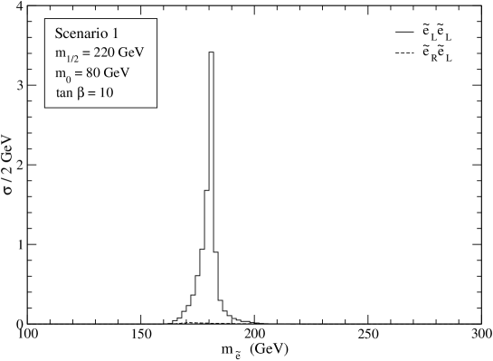
Figure 15: Reconstructed selectron mass in scenario 1, for $P_{1}=P_{2}=-0.8$.

Figure 16: Kinematical distribution of $E_{1}$ in scenario 1, for $P_{1}=P_{2}=-0.8$.

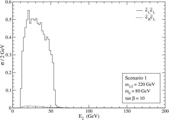
Figure 17: Kinematical distribution of $E_{2}$ in scenario 1, for $P_{1}=P_{2}=-0.8$.

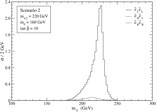
Figure 18: Reconstructed selectron masses in scenario 2, for $P_{1}=P_{2}=-0.8$.

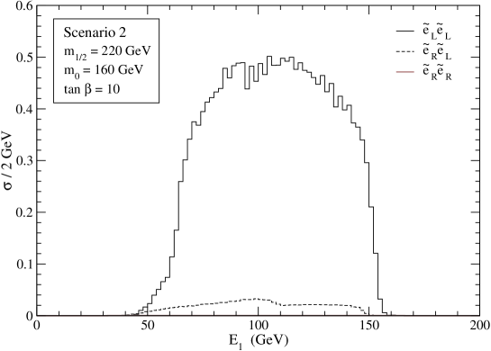
Figure 19: Kinematical distribution of $E_{1}$ in scenario 2, for $P_{1}=P_{2}=-0.8$.

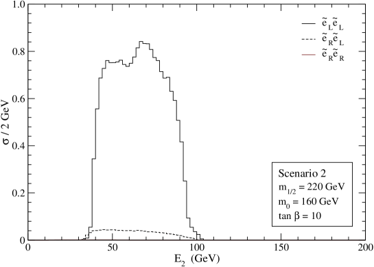
Figure 20: Kinematical distribution of $E_{2}$ in scenario 2, for $P_{1}=P_{2}=-0.8$.

B.2 Positive beam polarisation

Positive beam polarisation $P_{1}=P_{2}=0.8$ enhances the $\tilde{e}_{R}\tilde{e}_{R}$ signal by a factor of 3.24, reducing the $\tilde{e}_{L}\tilde{e}_{L}$ signal by a factor of 0.04 and the $\tilde{e}_{R}\tilde{e}_{L}$ background by 0.36. In scenario 1, positive beam polarisation does not offer any advantage, and we only present the plots for scenario 2, in Figs. 21–23.

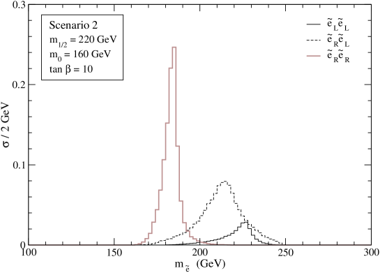
Figure 21: Reconstructed selectron masses in scenario 2, for $P_{1}=P_{2}=0.8$.

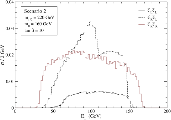
Figure 22: Kinematical distribution of $E_{1}$ in scenario 2, for $P_{1}=P_{2}=0.8$.

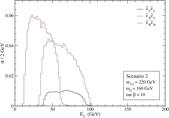
Figure 23: Kinematical distribution of $E_{2}$ in scenario 2, for $P_{1}=P_{2}=0.8$.

References

- [1] H. P. Nilles, Phys. Reports 110 (1984) 1
- [2] H. E. Haber and G. L. Kane, Phys. Reports 117 (1985) 75
- [3] S. P. Martin, in “Perspectives on supersymmetry”, G. L. Kane (ed.), hep-ph/9709356
- [4] ATLAS Detector and Physics Performance Technical Design Report, CERN-LHCC-99-14; S. Abdullin et al. [CMS Collaboration], J. Phys. G 28 (2002) 469
- [5] T. Kamon [CDF Collaboration], hep-ex/0301019
- [6] J. A. Aguilar-Saavedra et al. [ECFA/DESY LC Physics Working Group Collaboration], hep-ph/0106315
- [7] S. T. Petcov, Phys. Lett. B 139 (1984) 421
- [8] S. M. Bilenky, E. C. Christova and N. P. Nedelcheva, Bulg. J. Phys. 13 (1986) 283
- [9] G. Moortgat-Pick and H. Fraas, Eur. Phys. J. C 25 (2002) 189
- [10] J. L. Feng and M. E. Peskin, Phys. Rev. D 64 (2001) 115002
- [11] C. Blochinger, H. Fraas, G. Moortgat-Pick and W. Porod, Eur. Phys. J. C 24 (2002) 297
- [12] A. E. Nelson, N. Rius, V. Sanz and M. Unsal, JHEP 0208 (2002) 039
- [13] H. U. Martyn and G. A. Blair, hep-ph/9910416
- [14] J. L. Feng and D. E. Finnell, Phys. Rev. D 49 (1994) 2369
- [15] J. A. Aguilar-Saavedra and A. M. Teixeira, in preparation
- [16] J. Gluza and M. Zrałek, Phys. Lett. B 372 (1996) 259
- [17] E. Murayama, I. Watanabe and K. Hagiwara, KEK report 91-11, January 1992
- [18] A. Denner, H. Eck, O. Hahn and J. Küblbeck, Nucl. Phys. B 387 (1992) 467
- [19] A. Freitas and A. von Manteuffel, hep-ph/0211105
- [20] M. Skrzypek and S. Jadach, Z. Phys. C 49 (1991) 577
- [21] M. Peskin, Linear Collider Collaboration Note LCC-0010, January 1999
- [22] K. Yokoya and P. Chen, SLAC-PUB-4935. Presented at IEEE Particle Accelerator Conference, Chicago, Illinois, Mar 20-23, 1989
- [23] G. Alexander et al., TESLA Technical Design Report Part 4, DESY-01-011
- [24] R. Kleiss, W. J. Stirling and S. D. Ellis, Comput. Phys. Commun. 40 (1986) 359
- [25] A. H. Chamseddine, R. Arnowitt and P. Nath, Phys. Rev. Lett. 49 (1982) 970; R. Barbieri, S. Ferrara and C. A. Savoy, Phys. Lett. B 119 (1982) 343.
- [26] W. Porod, hep-ph/0301101
- [27] K. Hagiwara et al. [Particle Data Group Collaboration], Phys. Rev. D 66 (2002) 010001
- [28] A. Bartl, H. Fraas and W. Majerotto, Nucl. Phys. B 278 (1986) 1
- [29] A. Djouadi, Y. Mambrini and M. Mühlleitner, Eur. Phys. J. C 20 (2001) 563
- [30] See for instance J. R. Ellis, K. A. Olive, Y. Santoso and V. C. Spanos, hep-ph/0303043, and references therein
- [31] G. Degrassi, S. Heinemeyer, W. Hollik, P. Slavich and G. Weiglein, Eur. Phys. J. C 28 (2003) 133
- [32] H. U. Martyn, hep-ph/0002290
- [33] S. Y. Choi, J. Kalinowski, G. Moortgat-Pick and P. M. Zerwas, Eur. Phys. J. C 22 (2001) 563 [Addendum-ibid. C 23 (2002) 769]
- [34] S. Y. Choi, A. Djouadi, M. Guchait, J. Kalinowski, H. S. Song and P. M. Zerwas, Eur. Phys. J. C 14 (2000) 535
- [35] G. Moortgat-Pick, A. Bartl, H. Fraas and W. Majerotto, Eur. Phys. J. C 18 (2000) 379
-
[36]
J. C. Romão,
http://porthos.ist.utl.pt/romao/homepage/publications/
mssm-model/mssm-model.ps - [37] J. F. Gunion and H. E. Haber, Nucl. Phys. B 272 (1986) 1 [Erratum-ibid. B 402 (1993) 567]
- [38] J. F. Gunion, H. E. Haber, G. L. Kane and S. Dawson, “The Higgs Hunter’s Guide” (Perseus Publishing, Cambridge, MA, 1990)