Wess-Zumino-Witten term on the lattice

Abstract:

We construct the Wess-Zumino-Witten (WZW) term in lattice gauge theory by using a Dirac operator which obeys the Ginsparg-Wilson relation. Topological properties of the WZW term known in the continuum are reproduced on the lattice as a consequence of a non-trivial topological structure of the space of admissible lattice gauge fields. In the course of this analysis, we observe that the gauge anomaly generally implies that there is no basis of a Weyl fermion which leads to a single-valued expectation value in the fermion sector. The lattice Witten term, which carries information of a gauge path along which the gauge anomaly is integrated, is separated from the WZW term and the multivaluedness of the Witten term is shown to be related to the homotopy group $\pi_{2n+1}(G)$. We also discuss the global ${\rm SU}(2)$ anomaly on the basis of the WZW term.

1 Introduction

In continuum gauge theories in $d=2n$ dimensions, topological structures of the gauge theory and quantum anomalies are closely related. The configuration space of gauge fields defined on $S^{2n}$ is decomposed into an infinite number of connected components classified by the homotopy group $\pi_{2n-1}(G)$, where $G$ is the structure group of the gauge theory. By knowing the index of the Dirac operator, one can see to which connected component the background gauge field belongs. The quantum anomaly related to this topology of the gauge field is the axial anomaly [1]. Although each connected component $\mathcal{A}$ of the configuration space, being an affine space, is topologically trivial, the gauge orbit space $\mathcal{A}/\mathcal{G}$, where $\mathcal{G}$ is the group of gauge transformations, generically has a non-trivial topology. In particular, there may exist a non-contractible 2-sphere in the gauge orbit space which gives rise to a non-trivial $\pi_{2}(\mathcal{A}/\mathcal{G})=\pi_{1}(\mathcal{G})$. The latter implies the existence of a non-contractible loop in $\mathcal{G}$ and, when $G$ is simply-connected as we shall assume below, it is identical to the homotopy group $\pi_{2n+1}(G)$. Physically, the existence of a non-contractible 2-sphere in the gauge orbit space gives rise to an obstruction in defining a gauge invariant fermion determinant, i.e., the gauge anomaly [2].

In lattice gauge theory, any field configuration can smoothly be deformed into one another and, hence, the space of lattice gauge fields is intrinsically topologically trivial. However, it has been shown [3] that by imposing the admissibility condition

$$\|1-R[U(p)]\|<\epsilon,\qquad\hbox{for all plaquettes~{}$p$}\,,$$ (1)

where $U(p)$ is the product of link variables around the plaquette $p$ and $R$ stands for a unitary representation of the gauge group, it is possible to endow the space of lattice gauge fields with a non-trivial topological structure. The space of admissible lattice gauge fields is decomposed into a (finite) number of connected components and one can assign to each connected component $\mathfrak{U}$ a topological charge, which coincides with the Chern-Pontryagin index in the classical continuum limit [3]. For the overlap Dirac operator [4] which satisfies the Ginsparg-Wilson (GW) relation [5], the admissibility condition is required to guarantee the regularity of the Dirac operator [6]. Then the index of the Dirac operator, whose density is the axial anomaly on the lattice, is constant over $\mathfrak{U}$ due to the lattice index theorem [7, 4]. It is expected that the topological charge of ref. [3] and the index are identical when $\epsilon$ is sufficiently small [8].

A removal of non-admissible configurations from the space of gauge fields may leave “holes” in a connected component $\mathfrak{U}$. If this occurs, one may have non-trivial $\pi_{2}(\mathfrak{U})$ and this could cause, as we will see below, an obstruction in defining a smooth integration measure for Weyl fermions.

The basic picture behind a classification of topological sectors in lattice gauge theory however appears quite different from that in the continuum gauge theory. In the latter, the gauge potential approaches to a pure gauge configuration on the $2n-1$ dimensional sphere at infinity and this defines a mapping from the $2n-1$ sphere to $G$. The space of gauge potentials is thus classified by $\pi_{2n-1}(G)$. In lattice gauge theory, on the other hand, the admissibility (1) is a gauge invariant condition and does not place any restriction on gauge degrees of freedom. The space of lattice gauge transformations $\mathfrak{G}$ is topologically trivial even after imposing eq. (1). Hence the idea of classifying topological sectors of the gauge field by $\pi_{2n-1}(G)$ cannot be applied to lattice gauge theory as it stands. Similarly, on the lattice $\pi_{1}(\mathfrak{G})=0$ and the connection between a nontrivial $\pi_{1}(\mathcal{G})=\pi_{2n+1}(G)$ and the gauge anomaly seems to be lost in lattice gauge theory. This makes the construction of the Wess-Zumino-Witten (WZW) term [9, 10] in lattice gauge theory intricate because the multivalued nature of the WZW term in the continuum theory relies on the non-triviality of $\pi_{2n+1}(G)$.

In this paper, on the basis of a Dirac operator which obeys the GW relation, we formulate the WZW term on the lattice. Our WZW term is manifestly local on the lattice and has a correct classical continuum limit. Our construction can be regarded as an “anomalous version” of the formulation of refs. [11, 12] in which anomaly-free chiral gauge theories are studied. Our task is relatively simple compared to that for anomaly-free cases [11, 12] because we treat anomalous cases and it is not necessary to worry about the gauge anomaly cancellation on the lattice, which is a highly non-trivial issue. Unfortunately, however, our construction in its explicit form is applied only to a restricted class of gauge fields and gauge transformations and it may not be suitable for numerical simulations. Nevertheless, by using our construction, we can understand how various properties of the WZW term expected in the continuum on topological grounds are realized in the lattice framework, despite the above mentioned differences between the topology of gauge fields in continuum and lattice frameworks.

Our motivation is not new, and in fact, many related works can be found in the literature. Ref. [13] studied a construction of the WZW term in the context of Wilson fermion. The overlap formulation for lattice chiral gauge theories [14, 15] is closely related to the formulation of refs. [11, 12]. An implementation of the WZW term by the overlap has been proposed in ref. [15]. With the overlap formulation, the WZW term in 2-dimensions has been studied analytically and numerically [16]. To our knowledge, however, topological aspects of the WZW term on the lattice have not fully been investigated so far. In a later section, we will see that our WZW term on the lattice reproduces the winding number of the phase of chiral determinant along a gauge loop [2]. This is basically the result obtained in ref. [17] (in ref. [18], it was shown that the winding number can be expressed by the index of a Dirac operator in $2n+2$ dimensions). We will observe that a non-trivial winding number of chiral determinant, i.e, the gauge anomaly, is a consequence of non-contractible 2-spheres in $\mathfrak{U}$, which is classified by $\pi_{2n+1}(G)$. An existence of such non-contractible surfaces in $\mathfrak{U}$ has also been pointed out [19]. In the present paper, we show that a non-trivial winding number directly implies an obstruction in defining a smooth fermion measure, not only an obstruction for the gauge invariance; anomalous chiral gauge theories in general cannot consistently be formulated in the framework of refs. [11, 12]. Our way of argument to show this fact is simple and also provides a coherent picture to understand topological aspects of the WZW term.

This paper is organized as follows. Section 2 is devoted to a construction of the WZW term in lattice gauge theory, based on the Ginsparg-Wilson relation. Then, in section 3, we show that the WZW term exhibits an ambiguity of $2\pi$ multiple of an integer, depending on a choice of the gauge path along which the lattice gauge anomaly is integrated. We also show that this ambiguity can be separated as a term which does not depends on the gauge field (a lattice analogue of the Witten term [10]). In section 4, we study the winding number of the chiral determinant [2] and show that it is directly related to an obstruction to a smooth fermion measure. This shows that anomalous chiral gauge theories are intrinsically different from anomaly-free cases. In section 5, we show that the multivaluedness of the Witten term [10] is precisely realized on the lattice and its value is in fact classified by $\pi_{2n+1}(G)$. In section 6, on the basis of the result of ref. [23], we illustrate how the WZW term reproduces the global $\mathop{\rm SU}\nolimits(2)$ anomaly [24]. Section 7 is devoted to conclusion. In appendix A, we collect relevant materials for the classical continuum limit of the WZW term.

We consider $d=2n$ dimensional periodic lattice with a finite size. The lattice spacing will be denoted by $a$.

2 Construction of the WZW term

2.1 Basic idea

We first sketch our basic idea to define the WZW term on the lattice. We start with the chiral determinant of a (left-handed) Weyl fermion on the lattice

$$\det M[U]=\int{\rm D}[\psi]{\rm D}[\overline{\psi}]\,e^{-S_{\rm F}}\,,\qquad S_{\rm F}=a^{2n}\sum_{x}\overline{\psi}(x)D\psi(x)\,,$$ (2)

where $U$ denotes the lattice gauge field (link variables). In most part of this paper, we assume that the gauge field $U$ belongs to the vacuum sector. Namely, we assume that $U$ can smoothly be deformed into the trivial configuration $U=1$ within the space of admissible gauge fields specified by eq. (1); in eq. (1) $R$ stands for the gauge-group representation of the fermion.

In eq. (2), the Dirac operator $D$ is assumed to satisfy the GW relation

$$\gamma_{5}D+D\gamma_{5}=aD\gamma_{5}D\,.$$ (3)

Although we will not need the explicit form of $D$ in this paper, we assume following properties of $D$: The $\gamma_{5}$-hermiticity $D^{\dagger}=\gamma_{5}D\gamma_{5}$, the gauge covariance, the locality and absence of species doublers. These properties would imply the Dirac operator reproduces the correct axial anomaly in the classical continuum limit [25, 26]; we also assume this. Neuberger’s overlap Dirac operator [4] possesses all these properties if configurations of gauge field are restricted by the condition (1) [6]. Following refs. [27], we then introduce the modified chiral matrix $\hat{\gamma}_{5}=\gamma_{5}(1-aD)$, which fulfills

$$(\hat{\gamma}_{5})^{\dagger}=\hat{\gamma}_{5},\qquad(\hat{\gamma}_{5})^{2}=1\,,\qquad D\hat{\gamma}_{5}=-\gamma_{5}D$$ (4)

and define chiral projectors by

$$\hat{P}_{\pm}={1\over 2}(1\pm\hat{\gamma}_{5})\,,\qquad P_{\pm}={1\over 2}(1\pm\gamma_{5})\,,\qquad D\hat{P}_{\pm}=P_{\mp}D.$$ (5)

Then in eq. (2), the left-handed Weyl fermion is defined by imposing the constraints

$$\hat{P}_{-}\psi=\psi,\qquad\overline{\psi}=\overline{\psi}P_{+}\,.$$ (6)

In this construction, the chirality is consistently imposed due to the last relation of eq. (5). The action in eq. (2) is manifestly gauge invariant and consistent with the locality. We postpone the detailed account on the fermion measure ${\rm D}[\psi]{\rm D}[\overline{\psi}]$ of eq. (2) to the next subsection.

Assuming that the chiral determinant has been defined, we define the WZW term on the lattice by

$$i{\mit\Gamma}_{\rm WZW}[g,U]=\ln\det M[U]-\ln\det M[U^{g^{-1}}]\,,$$ (7)

where $U^{g}$ denotes the gauge transformation of the gauge field $U$ parametrized by $g$,

$$U^{g}(x,\mu)=g(x)U(x,\mu)g(x+a\hat{\mu})^{-1}\,.$$ (8)

From its definition, it is obvious that the WZW term vanishes if the chiral determinant is gauge invariant; it thus picks up only the effect of gauge anomaly. Under the infinitesimal gauge transformation,

$$\delta U(x,\mu) = \omega(x)U(x,\mu)-U(x,\mu)\omega(x+a\hat{\mu})=-a\nabla_{\mu}\omega(x)U(x,\mu)\,,$$

$$\delta g(x) = \omega(x)g(x)\,,$$ (9)

the combination $U^{g^{-1}}$ in the second term of eq. (7) does not change and, on the other hand, the first term produces the gauge anomaly. By this way, the WZW term, which will turn to be a local functional on the lattice, reproduces the gauge anomaly as $i\delta{\mit\Gamma}_{\rm WZW}[g,U]$ $=\delta\ln\det M[U]$. In the continuum theory, this is the defining relation of the WZW term.

2.2 Fermion integration measure and the associated $\mathop{\rm{}U}\nolimits(1)$ bundle

To define the fermion integration measure in eq. (2), we introduce an orthonormal complete set of vectors in the constrained space (6),

$$\hat{P}_{-}v_{j}=v_{j}\,,\qquad(v_{k},v_{j})=\delta_{kj}\,.$$ (10)

Note that $\sum_{j}v_{j}(x)v_{j}(y)^{\dagger}=\hat{P}_{-}(x,y)$. By expanding the fermion field in terms of this basis

$$\psi(x)=\sum_{j}v_{j}(x)c_{j}\,,$$ (11)

the integration measure is defined by

$${\rm D}[\psi]=\prod_{j}{\rm d}c_{j}\,.$$ (12)

Similarly, for the anti-fermion, by using a basis such that $\overline{v}_{k}P_{+}=\overline{v}_{k}$, we set

$${\rm D}[\overline{\psi}]=\prod_{k}{\rm d}\overline{c}_{k}\,,\qquad\overline{\psi}(x)=\sum_{k}\overline{c}_{k}\overline{v}_{k}(x)\,.$$ (13)

In terms of these bases, the chiral determinant (2) is given by the determinant of the matrix

$$M_{kj}=a^{2n}\sum_{x}\overline{v}_{k}(x)Dv_{j}(x)\,.$$ (14)

The above (seemingly simple) construction, however, poses complicated problems. First, the constraint (10) does not specify the basis vectors uniquely. A different choice of basis, as we will see shortly, leads to a difference in the phase of the fermion integration measure. This phase moreover may depend on the gauge field and hence may influence on the physical contents of the system. Secondly, a connected component of the space of admissible gauge fields $\mathfrak{U}$ can be topologically non-trivial as we already noted. Thus it is not obvious whether there exist bases over $\mathfrak{U}$, with which the chiral determinant (or more generally an expectation value of operators in the fermion sector) is a single-valued function over $\mathfrak{U}$. These closely related problems can be formulated as follows [11, 12].

We cover $\mathfrak{U}$ by local coordinate patches $X_{A}$, labeled by $A$. Suppose that some basis $v_{j}^{A}$ has been chosen within each patch, as is always possible for contractible local patches. Generally, however, on the intersection $X_{A}\cap X_{B}$ of two patches, basis vectors $v_{j}^{A}$ and $v_{j}^{B}$ are different and are related by a unitary transformation

$$v_{j}^{B}(x)=\sum_{k}v_{k}^{A}(x)\tau(A\to B)_{kj}\,.$$ (15)

By definition, the transition function $\tau(A\to B)$ satisfies the cocycle condition

$$\tau(A\to C)=\tau(A\to B)\tau(B\to C)\qquad\hbox{on $X_{A}\cap X_{B}\cap X_{C}$}$$ (16)

and thus defines a unitary principal bundle over $\mathfrak{U}$. Corresponding to eq. (15), the fermion integration measures defined in $X_{A}$ and in $X_{B}$ are related as

$${\rm D}[\psi]_{B}={\rm D}[\psi]_{A}g_{AB},\qquad g_{AB}=\det\tau(A\to B)\in\mathop{\rm{}U}\nolimits(1)\,.$$ (17)

This phase factor $g_{AB}$ thus defines a $\mathop{\rm{}U}\nolimits(1)$ bundle associated to the fermion integration measure. For a sensible formulation of Weyl fermions, various expectation values in the fermion sector must be a single-valued function over $\mathfrak{U}$. To realize this, one re-defines basis vectors in each patch such that $g_{AB}=1$ on all intersections. However, this is possible if and only if the $\mathop{\rm{}U}\nolimits(1)$ bundle is trivial.

To find a characterization of this $\mathop{\rm{}U}\nolimits(1)$ bundle, we consider a variation of gauge field

$$\delta_{\eta}U(x,\mu)=a\eta_{\mu}(x)U(x,\mu)\,,\qquad\eta_{\mu}(x)=\eta_{\mu}^{a}(x)T^{a}$$ (18)

and define the measure term within a patch, say $X_{A}$, by

$$\mathfrak{L}_{\eta}^{A}=i\sum_{j}(v_{j}^{A},\delta_{\eta}v_{j}^{A})\,.$$ (19)

This characterizes how the basis vectors change under the variation. On the intersection, $X_{A}\cap X_{B}$, we see from eq. (15) that the measure terms in $X_{A}$ and in $X_{B}$ are related as

$$\mathfrak{L}_{\eta}^{B}=\mathfrak{L}_{\eta}^{A}+ig_{AB}^{-1}\delta_{\eta}g_{AB}\,.$$ (20)

This shows that the measure term is the $\mathop{\rm{}U}\nolimits(1)$ connection associated to the $\mathop{\rm{}U}\nolimits(1)$ bundle. By applying the identity

$$\delta_{\eta}\delta_{\zeta}-\delta_{\zeta}\delta_{\eta}+a\delta_{[\eta,\zeta]}=0$$ (21)

to the definition of the measure term (19), we find

$$\delta_{\eta}\mathfrak{L}_{\zeta}^{A}-\delta_{\zeta}\mathfrak{L}_{\eta}^{A}+a\mathfrak{L}_{[\eta,\zeta]}^{A}=i\mathop{\rm Tr}\nolimits(\hat{P}_{-}[\delta_{\eta}\hat{P}_{-},\delta_{\zeta}\hat{P}_{-}])\,.$$ (22)

The right hand side, which depends neither on the patch label nor on basis vectors, is nothing but the curvature of the $\mathop{\rm{}U}\nolimits(1)$ bundle. Then as a measure of non-triviality of the $\mathop{\rm{}U}\nolimits(1)$ bundle, we may consider a 2-dimensional integral of the curvature, the first Chern number

$${1\over 2\pi}\int_{\mathcal{M}}{\rm d}t\,{\rm d}s\,i\mathop{\rm Tr}\nolimits(P_{t,s}[\partial_{t}P_{t,s},\partial_{s}P_{t,s}])\,,$$ (23)

which is an integer. $\mathcal{M}$ in this expression is a closed 2-surface in $\mathfrak{U}$ and $t$ and $s$ are local coordinates of $\mathcal{M}$. Namely, we defined two-parameter family of gauge fields $U_{t,s}$ in $\mathfrak{U}$, and accordingly defined the projection operators by $P_{t,s}=\hat{P}_{-}|_{U=U_{t,s}}$. If the above integer does not vanish, the $\mathop{\rm{}U}\nolimits(1)$ bundle is non-trivial and there exists no choice of basis vectors such that expectation values in the fermion sector are single-valued over $\mathcal{M}$. Namely, the Weyl fermion cannot consistently be formulated. In other words, $\mathcal{M}$ is a non-contractible 2-surface in $\mathfrak{U}$ which gives rise to a topological obstruction in defining a smooth fermion measure.

In the above argument, we started with basis vectors defined patch by patch. This way of argument, however, is not convenient in constructing the fermion measure which ensures the locality. The measure term $\mathcal{L}_{\eta}$, being linear in the variation $\eta$, can be expressed as

$$\mathcal{L}_{\eta}=a^{2n}\sum_{x}\eta_{\mu}^{a}(x)j_{\mu}^{a}(x)\,,$$ (24)

where $j_{\mu}^{a}(x)$ is termed the measure current. It can be shown [11] that the expected locality of the system is guaranteed if the measure current is a local function of link variables. To ensure the correct physical contents of the formulation, therefore, it is convenient to start with a certain local measure current. Then according to the reconstruction theorem [11, 12], if the local current satisfies the following conditions, one can re-construct basis vectors which lead to a smooth fermion measure that is consistent with the locality. The measure term (19) of the so constructed basis coincides with the measure term defined from the current by eq. (24). (1) The current is a smooth (i.e., single-valued) function of the gauge fields contained in $\mathfrak{U}$. (2) The measure term (24) defined from the current satisfies the global integrability

$$\exp\left(i\int_{0}^{1}{\rm d}t\,\mathcal{L}_{\eta}\right)=\det(1-P_{0}+P_{0}Q_{1})$$ (25)

along any closed loop in $\mathfrak{U}$. In this expression, the loop $U_{t}$ ($U_{1}=U_{0}$) is parametrized by $t\in[0,1]$ and the variation is given by $a\eta_{\mu}(x)=\partial_{t}U_{t}(x,\mu)U_{t}(x,\mu)^{-1}$. Projection operators along the loop are defined by $P_{t}=\hat{P}_{-}|_{U=U_{t}}$. The operator $Q_{t}$ is defined by the differential equation $\partial_{t}Q_{t}=[\partial_{t}P_{t},P_{t}]Q_{t}$ and $Q_{0}=1$. Thus the task to construct the fermion measure is reduced to find an appropriate local current $j_{\mu}^{a}(x)$ which satisfies the above two conditions. For an infinitesimally small (contractible) loop in $\mathfrak{U}$, it can be shown that the global integrability becomes the local integrability

$$\delta_{\eta}\mathfrak{L}_{\zeta}-\delta_{\zeta}\mathfrak{L}_{\eta}+a\mathfrak{L}_{[\eta,\zeta]}=i\mathop{\rm Tr}\nolimits(\hat{P}_{-}[\delta_{\eta}\hat{P}_{-},\delta_{\zeta}\hat{P}_{-}])$$ (26)

that is nothing but eq. (22) without patch labels (because here we started with a measure current defined globally over $\mathfrak{U}$). In this paper, we adopt this latter viewpoint which starts with the measure current and seek for an appropriate local measure current, or equivalently the measure term.

2.3 WZW term with the GW fermion

From the expression (14), we see that the infinitesimal variation of the chiral determinant is given by

$$\delta_{\eta}\ln\det M[U]=\mathop{\rm Tr}\nolimits(\delta_{\eta}D\hat{P}_{-}D^{-1}P_{+})-i\mathfrak{L}_{\eta}\,.$$ (27)

Therefore the WZW term (7) can be obtained by integrating this variation along a sequence of gauge transformations (a gauge path). We introduce a one-parameter family of gauge transformations

$$g_{t}(x),\qquad 0\leq t\leq 1$$ (28)

such that

$$g_{0}(x)=1,\qquad g_{1}(x)=g(x)\,.$$ (29)

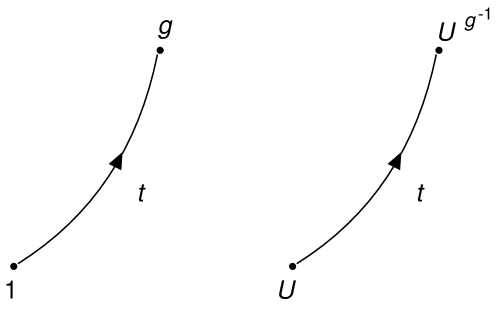
Figure 1: The paths in the space of gauge transformations (left) and in the space of gauge field configurations (right) along which we integrate a gauge variation of the chiral determinant to define the WZW term.

See figure 1. An example of such a path is given by

$$g_{t}(x)=[g(x)]^{t}.$$ (30)

In lattice gauge theory, such a smooth path $g_{t}$ which connects $1$ and $g$ always exists because $\pi_{0}(\mathfrak{G})=0$; the situation is quite different from the continuum. Corresponding to this path, we define a one-parameter family of gauge fields by

$$U_{t}(x,\mu)=U^{g_{t}^{-1}}(x,\mu),\qquad 0\leq t\leq 1\,,$$ (31)

which connects $U_{0}=U$ and $U_{1}=U^{g^{-1}}$ (figure 1). Note that, since the condition (1) is gauge invariant, if the starting configuration $U_{0}=U$ belongs to the space of admissible gauge fields $\mathfrak{U}$, then the path is also within $\mathfrak{U}$. By this way, we have

$${\mit\Gamma}_{\rm WZW}[g,U] = i\int_{0}^{1}{\rm d}t\,\partial_{t}\ln\det M[U^{g_{t}^{-1}}]$$ (32)

$$= i\int_{0}^{1}{\rm d}t\mathop{\rm Tr}\nolimits(\partial_{t}D\hat{P}_{-}D^{-1}P_{+})+\int_{0}^{1}{\rm d}t\,\mathfrak{L}_{\eta}\,,$$

where the variation in the second term is given by the gauge variation along the gauge path

$$\eta_{\mu}(x)=\nabla_{\mu}(g_{t}^{-1}\partial_{t}g_{t})(x)\,.$$ (33)

The first term of eq. (32) can be rendered manifestly local. Noting the gauge covariance of the Dirac operator

$$D|_{U=U_{t}}=R(g_{t}^{-1})D|_{U=U_{0}}R(g_{t})$$ (34)

and the last property of eq. (5), we have

$${\mit\Gamma}_{\rm WZW}[g,U]=a^{2n}\sum_{x}\mathcal{A}^{a}(x)|_{U}\int_{0}^{1}{\rm d}t\,(\partial_{t}g_{t}g_{t}^{-1})^{a}(x)+\int_{0}^{1}{\rm d}t\,\mathfrak{L}_{\eta}\,,$$ (35)

where the covariant gauge anomaly $\mathcal{A}^{a}(x)$ is defined by

$$\mathcal{A}^{a}(x)={ia\over 2}\mathop{\rm tr}\nolimits[\gamma_{5}R(T^{a})D(x,x)]\,.$$ (36)

This is a local function of gauge fields, because it does not contain the inverse of the Dirac operator which is generically a non-local combination of link variables.

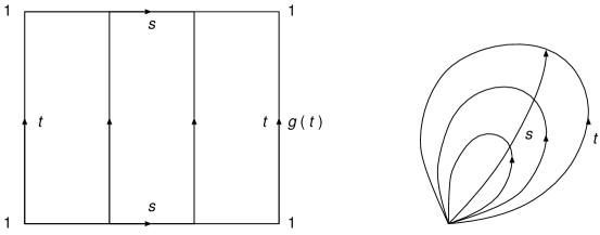
Figure 2: The two-parameter family of gauge transformations (left) and the two-parameter family gauge field configurations (right) utilized in eq. (43).

Now, the covariant gauge anomaly and the curvature in eq. (26) are not independent. To see this, take the gauge variation $\eta_{\mu}(x)=-\nabla_{\mu}\omega(x)$ as one variation in the curvature. Noting the gauge covariance $\delta_{\eta}\hat{P}_{-}=[R(\omega),\hat{P}_{-}]$ and the identity $\hat{P}_{-}\delta_{\zeta}\hat{P}_{-}\hat{P}_{-}=0$, we find

$$i\mathop{\rm Tr}\nolimits(\hat{P}_{-}[\delta_{\eta}\hat{P}_{-},\delta_{\zeta}\hat{P}_{-}])=-a^{2n}\sum_{x}\omega^{a}(x)\delta_{\zeta}\mathcal{A}^{a}(x)\,.$$ (37)

Namely, the curvature component in the direction of the gauge variation is given by a variation of the covariant anomaly. This relation is especially useful to find the classical continuum limit of the curvature, as we illustrate in appendix A. This relation also has an important consequence in our discussions below. Let us consider the case that the path (28) forms a closed loop, namely $g_{1}=g_{0}=1$. For this case, it is always possible to find a two-parameter family $g_{t,s}$ of gauge transformations such that

$$g_{0,s}(x)=g_{t,0}(x)=1\,,\qquad 0\leq t\leq 1,\quad 0\leq s\leq 1\,,$$ (38)

and

$$g_{t,1}(x)=g_{t}(x),\qquad 0\leq t\leq 1\,.$$ (39)

See figure 2. The example is

$$g_{t,s}(x)=[g_{t}(x)]^{s}\,.$$ (40)

Since these generate gauge transformations, the corresponding two-parameter family of gauge fields

$$U_{t,s}(x,\mu)=U^{g_{t,s}^{-1}}(x,\mu)\,,\qquad 0\leq t\leq 1,\quad 0\leq s\leq 1\,,$$ (41)

is within the space of admissible gauge fields $\mathfrak{U}$. Now we integrate the relation (37) over the disk represented in figure 2, by identifying $\eta$ as the gauge variation along the $t$-direction,

$$\eta_{\mu}(x)=\nabla_{\mu}(g_{t,s}^{-1}\partial_{t}g_{t,s})(x)$$ (42)

and $\zeta$ as the direction parametrized by $s$. Noting the gauge covariance of the covariant anomaly, we have

$$\int_{0}^{1}{\rm d}t\,a^{2n}\sum_{x}(g_{t}^{-1}\partial_{t}g_{t})^{a}(x)\mathcal{A}^{a}(x)|_{U=U_{t}} = a^{2n}\sum_{x}\mathcal{A}^{a}(x)|_{U=U_{0}}\int_{0}^{1}{\rm d}t\,(\partial_{t}g_{t}g_{t}^{-1})^{a}(x)$$ (43)

$$= i\int_{0}^{1}{\rm d}t\int_{0}^{1}{\rm d}s\,\mathop{\rm Tr}\nolimits(P_{t,s}[\partial_{t}P_{t,s},\partial_{s}P_{t,s}])\,,$$

where we have used the boundary conditions, eqs. (38) and (39). We have observed that, when the gauge path (31) is a closed loop in $\mathfrak{U}$, the first term of the WZW term (35) (a contribution of the covariant anomaly), can be expressed as the surface integral of the curvature over the disk (41) (this always exists within $\mathfrak{U}$) which is spanned by the loop. This property will be repeatedly utilized in the following discussions.

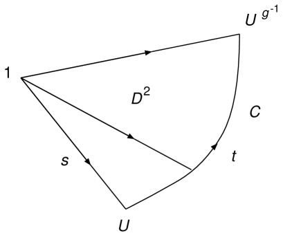
Figure 3: The two-parameter family of gauge field configurations to define the WZW term. The direction of $s$ is to construct the measure term (49) and the gauge anomaly is integrated along the gauge path $C$, the direction of $t$.

2.4 An explicit construction of the measure term

It is obvious that the above definition of the WZW term (35) is incomplete unless we provide an explicit form of the measure term $\mathfrak{L}_{\eta}$. To construct the measure term, we again consider a two-parameter family of gauge fields $U_{t,s}$, such that

$$U_{t,0}=1,\qquad 0\leq t\leq 1\,,$$ (44)

and

$$U_{t,1}=U^{g_{t}^{-1}}\,,\qquad 0\leq t\leq 1\,.$$ (45)

See figure 3. Here we encounter a trouble. There is no general guarantee that this family of gauge fields is contained in the space of admissible gauge fields, $\mathfrak{U}$. Recall that we have assumed that $U=U_{0,1}$ belongs to the vacuum sector. So the existence of a smooth path $U_{0,s}$ which connects $1$ and $U$ is guaranteed by assumption. However, the admissibility of general $U_{t,s}$ is not. In fact, in a later section, we will encounter an example in which such a smooth family does not exist. Thus to ensure the admissibility, we place following restrictions on $U$ and $g$; these limit an applicability of our construction. We assume that the gauge field $U$ is given by a lattice transcription of a certain gauge potential defined on a continuum torus $T^{2n}$. To be precise, link variables are given by the path-ordered exponential of a smooth gauge potential

$$U(x,\mu)=\mathcal{P}\exp\left[a\int_{0}^{1}{\rm d}u\,A_{\mu}(x+(1-u)a\hat{\mu})\right].$$ (46)

Also we assume that the gauge transformation parameter $g(x)$ is given by a lattice restriction of a certain smooth $G$-valued function defined on the torus. Under these restrictions, when the lattice spacing is sufficiently small, there always exists a two-parameter family of lattice gauge fields in $\mathcal{M}$ which possesses the above boundary values. For example, a choice

$$U_{t,s}(x,\mu)=[g_{t}^{-1}(x)U(x,\mu)g_{t}(x+a\hat{\mu})]^{s}$$ (47)

does the job.

With the above restrictions, it is easy to find an appropriate measure term. One way is to introduce an additional parameter $r$ and set $a\eta_{\mu}(x)=\partial_{t}U_{t,s,r}(x,\mu)U(x,\mu)_{t,s,r}^{-1}$ and $a\zeta_{\mu}(x)=\partial_{r}U(x,\mu)_{t,s,r}U(x,\mu)_{t,s,r}^{-1}$ in eq. (26) and then take a derivative of eq. (26) with respect to the parameter $s$. By noting the property $\mathop{\rm Tr}\nolimits(\delta_{1}\hat{P}_{-}\delta_{2}\hat{P}_{-}\delta_{3}\hat{P}_{-})=0$, one has

$$\partial_{t}\left[\partial_{s}\mathfrak{L}_{\zeta}-i\mathop{\rm Tr}\nolimits(P_{t,s,r}[\partial_{s}P_{t,s,r},\partial_{r}P_{t,s,r}])\right]-\partial_{r}\left[\partial_{s}\mathfrak{L}_{\eta}-i\mathop{\rm Tr}\nolimits(P_{t,s,r}[\partial_{s}P_{t,s,r},\partial_{t}P_{t,s,r}])\right]=0\,,$$ (48)

where $P_{t,s,r}=\hat{P}_{-}|_{U=U_{t,s,r}}$. A particular solution of this equation is given by $\partial_{s}\mathfrak{L}_{\eta}=i\mathop{\rm Tr}\nolimits(\hat{P}_{t,s,r}[\partial_{s}\hat{P}_{t,s,r},\partial_{t}\hat{P}_{t,s,r}])$. Then by getting rid of the parameter $r$ and integrating this relation along a direction of $s$ in figure 3, we have

$$\mathfrak{L}_{\eta}=i\int_{0}^{1}{\rm d}s\mathop{\rm Tr}\nolimits(P_{t,s}[\partial_{s}P_{t,s},\delta_{\eta}P_{t,s}])\,,$$ (49)

where $P_{t,s}=\hat{P}_{-}|_{U=U_{t,s}}$. Conversely, it is straightforward to verify that this measure term in fact satisfies the local integrability (26). This form of the measure term already appeared in refs. [11, 28]. This measure term is given by a combination of the Dirac operator and the corresponding measure current is a local function of link variables due to the locality of the Dirac operator. Thus it defines a sensible chiral determinant at least for configurations restricted as above.

The measure term (49) is yet ambiguous depending on the choice of the two-parameter family $U_{t,s}$. If we consider an infinitesimal deformation of the two-parameter family $\delta U_{t,s}$, we find the the measure term changes by

$$\delta\mathfrak{L}_{\eta}=i\delta_{\eta}\int_{0}^{1}{\rm d}s\mathop{\rm Tr}\nolimits(P_{t,s}[\partial_{s}P_{t,s},\delta P_{t,s}])\,.$$ (50)

By comparing this with the variation of the chiral determinant (27), we realize that this ambiguity is nothing but the standard ambiguity in defining the effective action, a freedom of choosing local counterterms (coboundary terms). To avoid this unimportant ambiguity, it is convenient to fix a convention for the two-parameter family $U_{t,s}$. Here we take eq. (47) as a part of definition of the WZW term. By this way, we have

$${\mit\Gamma}_{\rm WZW}[g,U]=a^{2n}\sum_{x}\mathcal{A}^{a}(x)|_{U}\int_{0}^{1}{\rm d}t\,(\partial_{t}g_{t}g_{t}^{-1})^{a}(x)-i\int_{0}^{1}{\rm d}t\int_{0}^{1}{\rm d}s\mathop{\rm Tr}\nolimits(P_{t,s}[\partial_{t}P_{t,s},\partial_{s}P_{t,s}])\,,$$ (51)

where $P_{t,s}=\hat{P}_{-}|_{U=U_{t,s}}$ and $U_{t,s}$ is defined by eq. (47). This completes our construction of the WZW term on the lattice. In appendix A, we show that this definition has the correct classical continuum limit.

The expression (51) can be cast into a parametrizaion free form as

$${\mit\Gamma}_{\rm WZW}[g,U]=-i\int_{C}\mathop{\rm Tr}\nolimits PD^{-1}P_{+}{\rm d}D-i\int_{D^{2}}\mathop{\rm Tr}\nolimits P{\rm d}P{\rm d}P\,,$$ (52)

where $D^{2}$ is the 2-disk $D^{2}$ in the space of admissible gauge fields parametrized by $t$ and $s$ as depicted in figure 3, $C$ is the path connecting $U$ and $U^{g^{-1}}$ parametrized by $t$ and ${\rm d}$ is the exterior derivative. The Dirac operator and the projector on the disk $D^{2}$ are simply denoted by $D$ and $P$. Since $C$ is a path along the gauge direction, the first term on the right hand side of (52) is local in the sense of lattice theory. As we shall show in the next section, the WZW term modulo $2\pi$ does not depend on the choice of $D^{2}$ as far as the two boundaries parametrized by $s$ are fixed and $C$ lies in the gauge direction.

By using eq. (51) and the relation $U^{(hg)^{-1}}=(U^{h^{-1}})^{g^{-1}}$, we find the composition law:

$${\mit\Gamma}_{\rm WZW}[hg,U]={\mit\Gamma}_{\rm WZW}[h,U]+{\mit\Gamma}_{\rm WZW}[g,U^{h^{-1}}]\pmod{2\pi}\,,$$ (53)

where the ambiguity of $2\pi$ will be explained in the next subsection (each WZW term in the above expression has such an ambiguity).

3 $2\pi$-ambiguity of the WZW term and the Witten term

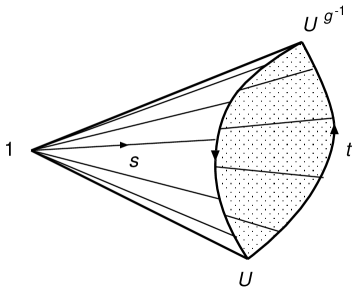
Figure 4: A difference between WZW terms defined with respect to two different gauge paths.

The WZW term (51) depends on a chosen gauge path $g_{t}$ through eq. (47) and this freedom of gauge path causes a $2\pi$-ambiguity of the WZW term. To show this, let us consider two gauge paths, $g_{t}^{(1)}$ and $g_{t}^{(2)}$. The difference between the WZW terms defined with respect to each path is obviously given by ${\mit\Gamma}_{\rm WZW}[1,U]$ in which the gauge path $g_{t}$ ($g_{0}=g_{1}=1$) is defined by

$$g_{t}(x)=\cases{g_{2t}^{(1)}(x)\,,&for $0\leq t\leq\displaystyle\frac{1}{2}$\,,\cr\cr g_{2(1-t)}^{(2)}(x)\,,&for $\displaystyle\frac{1}{2}\leq t\leq 1$\cr}$$ (54)

which forms a closed loop. See figure 4. However, we have observed in eq. (43) that, along a gauge loop, the line integral of the covariant anomaly in the WZW term is given by the surface integral of the curvature over a surface spanned by the loop. As a consequence, the difference is given by

$${\mit\Gamma}_{\rm WZW}[g,U]|_{g_{t}^{(1)}}-{\mit\Gamma}_{\rm WZW}[g,U]|_{g_{t}^{(2)}}=-\int_{S^{2}}{\rm d}t\,{\rm d}s\,i\mathop{\rm Tr}\nolimits(P_{t,s}[\partial_{t}P_{t,s},\partial_{s}P_{t,s}])\,,$$ (55)

here the integral is for a surface of the two dimensional cone depicted in figure 4, which is topologically a 2-sphere $S^{2}$. Note that an orientation of the coordinate system $(t,s)$ in figure 2 is opposite compared to that in figure 4. Here we adopt a convention that $(t,s)$ is the right-handed system. Thus the difference coincides with ($-2\pi$ times) the first Chern number (23) for the surface of the cone, $\mathcal{M}=S^{2}$. Therefore, even if the difference exists, it is a multiple of $2\pi$ and $\exp(i{\mit\Gamma}_{\rm WZW}[g,U])$ is a single valued functional of $g$ and $U$. If the Chern number is non-zero, the 2-sphere is non-contractible in the space of admissible gauge fields $\mathfrak{U}$. An important implication of this fact will be discussed in the next section.

Next we write the WZW term as

$${\mit\Gamma}_{\rm WZW}[g,U]={\mit\Gamma}_{\rm WZW}[g,U]-{\mit\Gamma}_{\rm WZW}[g,1]+{\mit\Gamma}_{\rm W}[g]\,,$$ (56)

where ${\mit\Gamma}_{\rm W}[g]={\mit\Gamma}_{\rm WZW}[g,1]$ will be referred to as the Witten term. The following simple argument shows that the part ${\mit\Gamma}_{\rm WZW}[g,U]-{\mit\Gamma}_{\rm WZW}[g,1]$ is free of the above $2\pi$-ambiguity. Namely it depends only on $g$ and $U$ and is ignorant about the “history” $g_{t}$ how $g$ evolved from $1$. The lattice Witten term ${\mit\Gamma}_{\rm W}[g]$, on the other hand, carries the $2\pi$-ambiguity and depends only on the gauge transformations $g_{t}$. To see these facts, let us consider how the WZW term ${\mit\Gamma}_{\rm WZW}[1,U]$ for a gauge loop $g_{t}$ ($g_{0}=g_{1}=1$) changes as we deform the gauge field $U$ to the trivial one, $U\to 1$. Defining a one-parameter family of gauge fields $U_{r}$ such that $U_{0}=U$ and $U_{1}=1$, at each value of the parameter $r$, we have a cone depicted figure 4 in which $U$ is replaced by $U_{r}$. The point is that everywhere of the surface of this cone is admissible by our assumption on $U$ and $g$ and, therefore, in ${\mit\Gamma}_{\rm WZW}[1,U]$ we can deform $U\to 1$ without encountering any violation of the admissibility. Since the Chern number, being an integer, is invariant under such a smooth deformation, the Chern numbers are identical for the two closed surfaces in figure 5. This implies that ${\mit\Gamma}_{\rm WZW}[g,U]$ and ${\mit\Gamma}_{\rm WZW}[g,1]$ has an identical $2\pi$-ambiguity; if one changes the path $g_{t}$, ${\mit\Gamma}_{\rm WZW}[g,U]$ and ${\mit\Gamma}_{\rm WZW}[g,1]$ exhibit an identical shift of $2\pi$. This shows the above assertions.

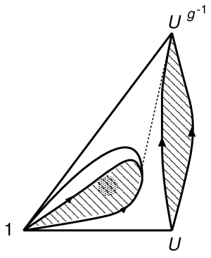
Figure 5: An integration of the curvature over the larger and the smaller closed surfaces gives rise to an integer multiple of $2\pi$ associated to an ambiguity of ${\mit\Gamma}_{\rm WZW}[g,U]$ and of ${\mit\Gamma}_{\rm WZW}[g,1]$ respectively. These two surfaces can be deformed to each other without encountering any violation of the admissibility. The shaded small circle contained in the smaller surface indicates a possible violation of the admissibility.

In the continuum theory, the WZW term is naturally decomposed into the $2n$ dimensional part, which depends only on the boundary values, $g$ and $U$, and the $2n+1$ dimensional Witten term, which does depend on $g_{t}$ but not on the gauge field, through the “homotopy formula” (87). It is interesting that our argument above performs this decomposition in effect, although we do not know a lattice analogue of the homotopy formula for the present.

4 Gauge anomaly and an obstruction for a smooth measure over $\mathfrak{U}$

Since information concerning the gauge anomaly is gathered in the WZW term, it is natural to examine the winding number of the phase of chiral determinant along a gauge loop [2] in our formulation. The winding number is obtained by considering a gauge loop $g_{t}$ such that $g_{0}=g_{1}=1$. Repeating the argument in the previous section, we have as the winding number

$${1\over 2\pi}{\mit\Gamma}_{\rm WZW}[1,U]=-{1\over 2\pi}\int_{S^{2}}{\rm d}t\,{\rm d}s\,i\mathop{\rm Tr}\nolimits(P_{t,s}[\partial_{t}P_{t,s},\partial_{s}P_{t,s}])\,,$$ (57)

where the integral is over a surface of the two dimensional cone (or $S^{2}$) depicted in figure 4. The above expression is nothing but the first Chern number (23) for $\mathcal{M}=S^{2}$ which is an integer. To see when this number becomes non-zero, it is enough to see the classical continuum limit, because it is an integer which cannot depend on the lattice spacing $a$. From eq. (89) in appendix A, we have

$${1\over 2\pi}{\mit\Gamma}_{\rm WZW}[1,U] = -{(-1)^{n}i^{n+1}n!\over(2\pi)^{n+1}(2n+1)!}\int_{S^{2n}\times S^{1}}{\rm d}^{2n+1}x\times$$ (58)

$$\times\,\epsilon_{\mu_{1}\mu_{2}\cdots\mu_{2n+1}}\mathop{\rm tr}\nolimits[R(g_{t}^{-1}\partial_{\mu_{1}}g_{t})R(g_{t}^{-1}\partial_{\mu_{2}}g_{t})\cdots R(g_{t}^{-1}\partial_{\mu_{2n+1}}g_{t})]\,.$$

The integrand is a total divergence and thus the integral is a homotopy invariant of the mapping $g_{t}(x)$ from $S^{2n}\times S^{1}$ to the gauge group $G$. However, since $G$ is simply-connected, the homotopy class is identical to that of mappings from the sphere $S^{2n+1}$ to $G$ [2]. Therefore, when the mapping $g_{t}(x)$ corresponds to a non-trivial element of $\pi_{2n+1}(G)$, the above winding number may become non-zero, depending on the representation $R$. A non-trivial $\pi_{2n+1}(G)$ is a measure for the gauge anomaly in the continuum theory [2]. These are basically observations already made in refs. [18, 17].

Our argument, however, shows that the gauge anomaly has a profound implication in the present lattice formulation. Eq. (57) says that when the winding number, which is a measure of the gauge anomaly, is non-zero, the Chern number (23) defined for a surface of the cone in figure 4 becomes non-zero. This implies that the $\mathop{\rm{}U}\nolimits(1)$ bundle associated to the fermion measure is non-trivial and, as we discussed in section 2.2, and the Weyl fermion cannot consistently be formulated, even if one sacrifices the gauge invariance. This shows that anomalous cases are completely different from anomaly-free cases from a view point of the present lattice formulation based on the GW relation. It seems interesting to re-examine quantization of anomalous gauge theories [32] in light of this observation.

5 Witten term and the multivaluedness

Figure 6: The two different paths to define the Witten term in the space of gauge transformations (left) and in the space of gauge field configurations (right). A difference between the Witten terms is given by an integral of the curvature over the closed surface in the right-hand figure.

We defined the Witten term by

$${\mit\Gamma}_{\rm W}[g]={\mit\Gamma}_{\rm WZW}[g,1]\,.$$ (59)

According to an understanding in the continuum theory [10], this term should have an ambiguity of $2\pi$ (multivaluedness) in a somewhat different sense from what we discussed so far. The key observation is that when $U=1$, the choice of the gauge path (28) has a wider freedom. Let $g_{*}$ be a constant $G$-transformation. Since $1^{g_{*}}=1$, one can use $g_{t}(x)$ which has the boundary values

$$g_{0}(x)=g_{*},\qquad g_{1}(x)=g(x)\,,$$ (60)

instead of eq. (29) in defining of ${\mit\Gamma}_{\rm W}[g]$. Then in the space of gauge transformations, we consider two paths, one starts from $1$ and ends at $g$ and another starts from $g_{*}$ and ends with $g$. See figure 6. We can then consider a difference between the Witten terms defined by each path. This is given by the Witten term defined by a path in the space of gauge transformations, which starts at $1$ and ends at $g_{*}$. In the space of gauge fields, this path corresponds to a loop. Even with the above change (60), our arguments so far hold with trivial changes. For example, $1$ in the right hand bottom corner of the square in figure 2 is replaced by $g_{*}$. The relation (43) for a loop holds as it stands and, by a similar argument as above, we have

$${\mit\Gamma}_{\rm W}[g]|_{1}-{\mit\Gamma}_{\rm W}[g]|_{g_{*}}=-\int_{S^{2}}{\rm d}t\,{\rm d}s\,i\mathop{\rm Tr}\nolimits(P_{t,s}[\partial_{t}P_{t,s},\partial_{s}P_{t,s}])\,,$$ (61)

where we have indicated the initial value in two gauge paths. This is an integer multiple of $2\pi$ because it is given by the Chern number (23). The explicit value of this difference can be found by the classical continuum limit

$${\mit\Gamma}_{\rm W}[g]|_{1}-{\mit\Gamma}_{\rm W}[g]|_{g_{*}} = -{(-1)^{n}i^{n+1}n!\over(2\pi)^{n}(2n+1)!}\int_{S^{2n}\times I}{\rm d}^{2n+1}x\times$$ (62)

$$\times\,\epsilon_{\mu_{1}\mu_{2}\cdots\mu_{2n+1}}\mathop{\rm tr}\nolimits[R(g_{t}^{-1}\partial_{\mu_{1}}g_{t})R(g_{t}^{-1}\partial_{\mu_{2}}g_{t})\cdots R(g_{t}^{-1}\partial_{\mu_{2n+1}}g_{t})]\,,\qquad$$

where the boundary condition along the interval $I$ is such that $g_{0}=1$ and $g_{1}=g_{*}$. Then the picture in figure 7 emerges. Namely, the difference is given by ($-2\pi$ times) a winding number of the mapping $g_{t}(x)$ which wraps around a basic $2n+1$ dimensional basic sphere in $G$ [10]. By this way, a non-trivial $\pi_{2n+1}(G)$ implies the multivaluedness of the Witten term on the lattice by $2\pi$, as in the continuum [10].

Figure 7: The image of the mapping $g_{t}(x)$ from $S^{2n}\times I$ to $G$ in eq. (62). Each latitude corresponds to the image of $g_{t}(x)$ at each $t$. The integral (62) is the winding number on this $2n+1$ dimensional sphere in $G$.

6 Global $\mathop{\rm SU}\nolimits(2)$ anomaly

As the final application of the WZW term, we consider the global $\mathop{\rm SU}\nolimits(2)$ anomaly [24] in lattice gauge theory [29, 23]. We assume that $d=2n=4$ and the Weyl fermion belongs to the fundamental ${1\over 2}$ representation of $\mathop{\rm SU}\nolimits(2)$. Since $\pi_{4}(\mathop{\rm SU}\nolimits(2))=Z_{2}$, there exists one homotopy class of gauge transformations in the continuum theory which cannot smoothly be deformed into the identity. Let $g(x)$ be such a homotopically non-trivial gauge transformation. In the continuum theory, Witten showed that the chiral determinant for $A^{g}$, the gauge transformation of the vector potential $A$, has a different sign compared to that for $A$. This implies ${\mit\Gamma}_{\rm WZW}[g,U]=\pi\bmod 2\pi$ in terms of the WZW term.

In the present case, since the fundamental representation of $\mathop{\rm SU}\nolimits(2)$ is pseudo-real, we have

$$\mathcal{A}^{a}(x)=0\,,\qquad i\mathop{\rm Tr}\nolimits(\hat{P}_{-}[\delta_{\eta}\hat{P}_{-},\delta_{\zeta}\hat{P}_{-}])=0\,.$$ (63)

So if our construction (51) is applicable to this case, we would conclude ${\mit\Gamma}_{\rm WZW}[g,U]=0$ which does not reproduce the $\mathop{\rm SU}\nolimits(2)$ anomaly. In fact, our construction breaks down due to a non-contractible loop in the space of admissible gauge fields $\mathfrak{U}$ [23]. The point is that each configuration on intermediate points of the gauge path (28), where $g$ is given by a lattice restriction of the continuum $g$, does not have a continuum counterpart, because $g$ in the continuum is not homotopically equivalent to the identity. This implies that there is no guarantee that the whole disk in figure 3 is contained in $\mathfrak{U}$. In fact, the analysis of ref. [23] shows that there must be a “hole” on the disk. The contribution of this hole must be taken into account to pick up the correct phase in the WZW term (a situation analogous to the Aharanov-Bohm effect).

This difficulty can be evaded by enlarging the gauge group $\mathop{\rm SU}\nolimits(2)$ to a larger group $G$ for which $\pi_{4}(G)=0$, say $G=\mathop{\rm SU}\nolimits(3)$. We then consider the fundamental representation of $\mathop{\rm SU}\nolimits(3)$ and embed the fundamental representation of $\mathop{\rm SU}\nolimits(2)$ as [10, 30, 23]

$$\Omega(x)=\pmatrix{g(x)&0\cr 0&1\cr}\in\mathop{\rm SU}\nolimits(3).$$ (64)

Since $\pi_{4}(\mathop{\rm SU}\nolimits(3))=0$, there exists a one-parameter family of $\mathop{\rm SU}\nolimits(3)$ gauge transformations in the continuum theory which interpolates $1$ and $\Omega(x)$. The lattice transcription of these $\mathop{\rm SU}\nolimits(3)$ gauge transformations thus provides a gauge path $\Omega_{t}(x)$ such that $\Omega_{0}(x)=1$ and $\Omega_{1}(x)=\Omega(x)$ and each point of $\Omega_{t}(x)$ has the continuum counterpart. Therefore our construction of the WZW term can be applied along this gauge path $\Omega_{t}(x)$ in $\mathop{\rm SU}\nolimits(3)$ lattice theory. See figure 8.

Figure 8: A way to construct the WZW term corresponding to a fundamental fermion of $\mathop{\rm SU}\nolimits(2)$. We can apply our construction of the measure term and the WZW term along the gauge path of $\mathop{\rm SU}\nolimits(3)$, $\Omega_{t}$ (the broken line). The measure term for the $\mathop{\rm SU}\nolimits(2)$ gauge path $g_{t}$ (the straight line) is defined by extending the $s$-integration along the gauge surface spanned by two gauge paths. Then the WZW term defined with respect to the $\mathop{\rm SU}\nolimits(2)$ gauge path is obtained. These two WZW terms, however, are identical.

In the $\mathop{\rm SU}\nolimits(3)$ theory, we then have two gauge paths, one is nothing but $g_{t}$ trivially embedded in the $\mathop{\rm SU}\nolimits(3)$ theory and another is given by $\Omega_{t}$. As shown in figure 8, within the $\mathop{\rm SU}\nolimits(3)$ theory, we can provide measure terms for those two gauge paths and define the WZW term along each of them. However, by repeating an argument similar to that of section 3, we can see that a difference between those two WZW terms is zero. Thus we define the WZW term corresponding to a fundamental fermion of $\mathop{\rm SU}\nolimits(2)$, ${\mit\Gamma}_{\rm WZW}[g,U]$ by using eqs. (51) and (47) with the replacement $g_{t}\to\Omega_{t}$.

We next show that

$${\mit\Gamma}_{\rm WZW}[g,U]={\mit\Gamma}_{\rm WZW}[g,1]={\mit\Gamma}_{\rm W}[g]\,.$$ (65)

To show this, we introduce a one-parameter family of $\mathop{\rm SU}\nolimits(2)$ gauge fields $U_{r}$ such that $U_{0}=U$ and $U_{1}=1$ and consider ${\mit\Gamma}_{\rm WZW}[g,U_{r}]$. According to our construction of the WZW term, ${\mit\Gamma}_{\rm WZW}[g,U_{r}]$ is given by an integral of the curvature over a surface $\mathcal{S}_{r}$ whose vertices are $1$, $U_{r}$ and $U_{r}^{g^{-1}}$, as depicted in figure 8 for $r=0$. We note that all configurations on these surfaces $\mathcal{S}_{r}$ are admissible for every $r$. We can therefore deform the surface $\mathcal{S}_{0}$, to that for $r=1$, $\mathcal{S}_{1}$, without encountering any violation of the admissibility as depicted in figure 9. These facts show that a difference between the WZW terms, ${\mit\Gamma}_{\rm WZW}[g,U]$ and ${\mit\Gamma}_{\rm WZW}[g,1]$, is given by an integral of the curvature over a surface $\mathcal{R}$ which is swept by the boundary of $\mathcal{S}_{r}$ in the process of the above deformation (the shaded area of figure 9), because $\mathcal{S}_{0}$, $\mathcal{S}_{1}$ and $\mathcal{R}$ form a closed 2-surface and within the closed surface there is no violation of the admissibility. However, the integral of the curvature over $\mathcal{R}$ vanishes because configurations on $\mathcal{R}$ act on the fundamental representation of $\mathop{\rm SU}\nolimits(3)$ as ${1\over 2}\otimes 1$ representation of $\mathop{\rm SU}\nolimits(2)$ and for such a representation, the curvature vanishes as eq. (63) shows. This argument establishes eq. (65).

Figure 9: Surfaces $\mathcal{S}_{0}$ and $\mathcal{S}_{1}$, and the region $\mathcal{R}$ (the shaded area) which is swept by the boundary of $\mathcal{S}_{r}$, utilized to show eq. (65).

By a similar deformation argument, one can see that

$${\mit\Gamma}_{\rm WZW}[g,U]={\mit\Gamma}_{\rm WZW}[h,U],$$ (66)

as long as $g$ and $h$ are given by a lattice restriction of homotopically equivalent $\mathop{\rm SU}\nolimits(2)$ gauge transformations $g(x)$ and $h(x)$ in the continuum.

The above two properties of the WZW term, combined with the classical continuum limit, show that ${\mit\Gamma}_{\rm WZW}[g,U]=\pi\bmod 2\pi$. We first note that $g(x)^{2}$ in the continuum belongs to a trivial homotopy class and according to eqs. (65) and (66),

$${\mit\Gamma}_{\rm WZW}[g^{2},U]={\mit\Gamma}_{\rm WZW}[1,U]={\mit\Gamma}_{\rm W}[1]=0\pmod{2\pi}\,,$$ (67)

where the last equality follows from the argument of section 3. On the other hand, from the composition law (53) and eq. (65), we have

$${\mit\Gamma}_{\rm WZW}[g^{2},U] = {\mit\Gamma}_{\rm WZW}[g,U]+{\mit\Gamma}_{\rm WZW}[g,U^{g^{-1}}]\pmod{2\pi}$$ (68)

$$= 2{\mit\Gamma}_{\rm W}[g]\pmod{2\pi}\,.$$

Then from eqs. (67) and (68), we infer that possible values of the WZW term are quantized even on the lattice as ${\mit\Gamma}_{\rm WZW}[g,U]={\mit\Gamma}_{\rm W}[g]=0\bmod 2\pi$ or ${\mit\Gamma}_{\rm WZW}[g,U]={\mit\Gamma}_{\rm W}[g]=\pi\bmod 2\pi$. One can decide which is actually the case from the classical continuum limit (90)

$${\mit\Gamma}_{\rm W}[g]={i\over 240\pi^{2}}\int_{S^{4}\times I}{\rm d}^{5}x\,\epsilon_{\mu\nu\rho\sigma\lambda}\mathop{\rm tr}\nolimits[R(\Omega_{t}^{-1}\partial_{\mu}\Omega_{t})R(\Omega_{t}^{-1}\partial_{\nu}\Omega_{t})\cdots R(\Omega_{t}^{-1}\partial_{\lambda}\Omega_{t})]+O(a)\,,$$ (69)

where $R$ stands for the fundamental representation of $\mathop{\rm SU}\nolimits(3)$. According to ref. [31], the above integral is $\pi\bmod 2\pi$ and thus ${\mit\Gamma}_{\rm WZW}[g,U]=\pi\bmod 2\pi$. By this way, the lattice Witten term reproduces the $\mathop{\rm SU}\nolimits(2)$ anomaly.

7 Conclusion

In this paper, we have formulated the WZW term in lattice gauge theory on the basis of a Dirac operator which satisfies the GW relation. We observed that topological properties of the WZW term in the continuum are neatly reproduced in the lattice framework, although a basic mechanism is rather different: In our formulation, a non-trivial topology of (a connected component of) the configuration space of lattice gauge fields due to the admissibility is the key element. On the other hand, (a connected component of) the configuration space of gauge fields in the continuum is topologically trivial. An important observation which emerged through our analysis is that it is generically impossible to formulate a Weyl fermion in an anomalous gauge-group representation, along the line of refs. [11, 12], because for such a representation, the Chern number (57) may become non-zero. If this occurs, a smooth fermion measure does not exist even the gauge invariance is sacrificed. With this observation, it seems interesting to re-examine a quantization of anomalous chiral gauge theories [32] within the lattice framework on the basis of the GW relation.

Appendix A Classical continuum limit

The lattice transcription (46) of a continuum gauge field is assumed in taking the classical continuum limit. To write down various quantities in the continuum limit, a use of differential form is quite helpful. The gauge potential 1-form and the field strength 2-form are defined respectively by

$$A=A_{\mu}{\rm d}x_{\mu}\,,\qquad F={\rm d}A+A^{2}={1\over 2}F_{\mu\nu}{\rm d}x_{\mu}{\rm d}x_{\nu}$$ (70)

from a gauge field in the continuum theory. The exterior derivative ${\rm d}$ is defined by ${\rm d}={\rm d}x_{\mu}\,\partial/(\partial x_{\mu})$.

It is not so difficult to explicitly evaluate the continuum limit of the covariant anomaly (36) for the overlap-Dirac operator [25]. For an evaluation in arbitrary even dimensions, see ref. [26]. By multiplying the volume form ${\rm d}^{2n}x={\rm d}x_{1}\cdots{\rm d}x_{2n}$, the continuum limit is given by

$$\mathcal{A}^{a}(x)\,{\rm d}^{2n}x=c_{1}\mathop{\rm tr}\nolimits[T^{a}F(x)^{n}]+O(a)\,,$$ (71)

where

$$c_{1}=-{i^{n+1}\over(2\pi)^{n}n!}\,.$$ (72)

On the other hand, an explicit evaluation of the continuum limit of the curvature $i\mathop{\rm Tr}\nolimits(\hat{P}_{-}[\delta_{\eta}\hat{P}_{-},\delta_{\zeta}\hat{P}_{-}])$ is more involved, although executable [17]. Here we invoke a general argument [12] which immediately leads to the answer. If the variations $\eta_{\mu}(x)$ and $\zeta_{\mu}(x)$ are lattice restrictions of some smooth vector fields in the continuum, the locality and symmetries of the curvature imply that a general form of the continuum limit is given by

$$i\mathop{\rm Tr}\nolimits(\hat{P}_{-}[\delta_{\eta}\hat{P}_{-},\delta_{\zeta}\hat{P}_{-}])=c_{2}\int_{T^{2n}}\mathop{\rm str}\nolimits(\eta\zeta F^{n-1})+O(a)\,,$$ (73)

where $\eta=\eta_{\mu}{\rm d}x_{\mu}$, $\zeta=\zeta_{\mu}{\rm d}x_{\mu}$ and $\mathop{\rm str}\nolimits$ denotes the symmetrized trace [33] defined by

$$\mathop{\rm str}\nolimits(A_{1}A_{2}\cdots A_{n})=\sum_{\sigma}{1\over n!}\epsilon_{\sigma}\mathop{\rm tr}\nolimits(A_{\sigma(1)}A_{\sigma(2)}\cdots A_{\sigma(n)})\,.$$ (74)

In this expression, the summation is taken over all permutations $\sigma$ and $\epsilon_{\sigma}$ is the parity associated to the permutation $\sigma$, $A_{1}A_{2}\cdots A_{n}\to A_{\sigma(1)}A_{\sigma(2)}\cdots A_{\sigma(n)}$, regarding odd rank forms as an anti-commuting quantity. Then by putting eqs. (71) and (73) into eq. (37), where $\eta=-{\rm d}\omega-[A,\omega]+O(a)$ and $\delta_{\zeta}A=\zeta+O(a)$ in the continuum limit, we find

$$c_{2}=-nc_{1}$$ (75)

by using the Bianchi identity

$${\rm d}F+[A,F]=0\,.$$ (76)

In the continuum limit, the two parameter family of the gauge fields (47) corresponds to a family of the gauge potentials

$$A_{t,s}=sA^{g_{t}^{-1}}+O(a),\qquad A^{g_{t}^{-1}}=g_{t}^{-1}({\rm d}+A)g_{t}\,.$$ (77)

Then in eq. (51), a contribution of the covariant anomaly to the WZW term ${\mit\Gamma}_{\rm WZW}$ becomes

$$c_{1}\int_{T^{2n}}\int_{0}^{1}{\rm d}t\,\mathop{\rm tr}\nolimits(g_{t}^{-1}\partial_{t}g_{t}F^{n})|_{A=A^{g_{t}^{-1}}}+O(a)\,.$$ (78)

On the other hand, the contribution of the measure term is given by substituting

$$\eta = \partial_{t}A_{t,s}=s[{\rm d}(g_{t}^{-1}\partial_{t}g_{t})+[A^{g_{t}^{-1}},g_{t}^{-1}\partial_{t}g_{t}]],$$

$$\zeta = \partial_{s}A_{t,s}=A^{g_{t}^{-1}},$$

$$F = {\rm d}A_{t,s}+A_{t,s}^{2}=F_{s}|_{A=A^{g_{t}^{-1}}}\,,\qquad F_{s}=s{\rm d}A+s^{2}A^{2}$$ (79)

in eq. (73) as

$$c_{1}\int_{T^{2n}}\int_{0}^{1}{\rm d}t\,n\int_{0}^{1}{\rm d}s\,s\mathop{\rm str}\nolimits\{[{\rm d}(g_{t}^{-1}\partial_{t}g_{t})+[A,g_{t}^{-1}\partial_{t}g_{t}]]AF_{s}^{n-1}\}|_{A=A^{g_{t}^{-1}}}+O(a)\,.$$ (80)

The integrand is the covariant divergence of the Bardeen-Zumino current [34] which supplies a difference between the consistent anomaly and the covariant anomaly. We note that eq. (78) can be written as

$$c_{1}\int_{T^{2n}}\int_{0}^{1}{\rm d}t\int_{0}^{1}{\rm d}s\,{\partial\over\partial s}\mathop{\rm str}\nolimits(g_{t}^{-1}\partial_{t}g_{t}F_{s}^{n})|_{A=A^{g_{t}^{-1}}}+O(a)\,.$$ (81)

Then by using the Bianchi identity ${\rm d}F_{s}+s[A,F_{s}]=0$, as a sum of eqs. (80) and (81), we have

$${\mit\Gamma}_{\rm WZW}[g,U]={c_{1}\over n+1}\int_{T^{2n}\times I}\omega_{2n}^{1}(g_{t}^{-1}{\rm d}_{t}g_{t},A^{g_{t}^{-1}})+O(a)\,,\qquad{\rm d}_{t}={\rm d}t\,{\partial\over\partial t}\,,$$ (82)

where the interval $I=[0,1]$ stands for the integration region of $t$. The consistent anomaly $\omega_{2n}^{1}$ in this expression is defined by

$$\omega_{2n}^{1}(C,A)=n(n+1)\int_{0}^{1}{\rm d}s\,(1-s)\mathop{\rm str}\nolimits[C{\rm d}(AF_{s}^{n-1})]\,.$$ (83)

Eq. (82) is the standard expression of the WZW term in the continuum (i.e., the integrated anomaly) and establishes that our construction (51) has the correct continuum limit. The following is merely a copy of the standard argument in the continuum [35].

Eq. (82) can be written in a $2n+1$ dimensional form by using the Chern-Simons form $\omega_{2n+1}$ as

$${\mit\Gamma}_{\rm WZW}[g,U]={c_{1}\over n+1}\int_{T^{2n}\times I}\omega_{2n+1}(\mathcal{A}^{g_{t}^{-1}},\mathcal{F}^{g_{t}^{-1}})+O(a)\,,$$ (84)

where the Chern-Simons form is defined by

$$\omega_{2n+1}(A,F)=(n+1)\int_{0}^{1}{\rm d}s\,\mathop{\rm tr}\nolimits(AF_{s}^{n})$$ (85)

and $\mathcal{A}^{g_{t}^{-1}}$ and $\mathcal{F}^{g_{t}^{-1}}$ are gauge fields extended to $2n+1$ dimensions by using the gauge transformation:

$$\mathcal{A}^{g_{t}^{-1}}=g_{t}^{-1}({\rm d}+{\rm d}_{t}+A)g_{t}\,,\qquad\mathcal{F}^{g_{t}^{-1}}=g_{t}^{-1}Fg_{t}\,.$$ (86)

The gauge transformation law of the Chern-Simons form is well-known [35]:

$$\omega_{2n+1}(\mathcal{A}^{g_{t}^{-1}},\mathcal{F}^{g_{t}^{-1}})=\omega_{2n+1}(A,F)+({\rm d}+{\rm d}_{t})\alpha_{2n}+\omega_{2n+1}(g_{t}^{-1}({\rm d}+{\rm d}_{t})g_{t},0)\,.$$ (87)

For lower dimensions, the explicit form of $\alpha_{2n}$ is given by

$$\alpha_{2}(V,A) = -\mathop{\rm tr}\nolimits(VA),$$

$$\alpha_{4}(V,A) = -{1\over 2}\mathop{\rm tr}\nolimits\left[V(A{\rm d}A+{\rm d}AA+A^{3})-{1\over 2}VAVA-V^{3}A\right],$$ (88)

where $V={\rm d}gg^{-1}$. For higher dimensions, $\alpha_{2n}$ can systematically be constructed by using Cartan’s homotopy formula [35]. By substituting eq. (87) in eq. (84) and by noting that the $2n+1$ dimensional integral of $\omega_{2n+1}(A,F)$ vanishes (because it does not contain ${\rm d}t$), we have

$${\mit\Gamma}_{\rm WZW}[g,U] = {c_{1}\over n+1}\int_{T^{2n}}\alpha_{2n}(V={\rm d}gg^{-1},A)$$ (89)

$$+\,{(-1)^{n}(n!)^{2}c_{1}\over(2n+1)!}\int_{T^{2n}\times I}\mathop{\rm tr}\nolimits[g_{t}^{-1}({\rm d}+{\rm d}_{t})g_{t}]^{2n+1}+O(a)\,.$$

In particular, the classical continuum limit of the Witten term ${\mit\Gamma}_{\rm W}[g]={\mit\Gamma}_{\rm WZW}[g,1]$ is given by

$${\mit\Gamma}_{\rm W}[g]=-{(-1)^{n}i^{n+1}n!\over(2\pi)^{n}(2n+1)!}\int_{T^{2n}\times I}\mathop{\rm tr}\nolimits[g_{t}^{-1}({\rm d}+{\rm d}_{t})g_{t}]^{2n+1}+O(a)\,.$$ (90)

Note added in proofs.

The interpolations with respect to the parameter $s$ in eqs. (40) and (47) are not uniquely defined when “exceptional configurations” appear within the power. For example, $-1$ is an element of $\mathop{\rm SU}\nolimits(N)$ with even $N$ and $(-1)^{s}$ is not uniquely defined. If this situation happens, we deform the one-parameter family $g_{t}(x)$ infinitesimally so that only non-exceptional configurations appear in the power. We thank David H. Adams for a comment on this point.

References

- [1] K. Fujikawa, Path integral measure for gauge invariant fermion theories, Phys. Rev. D 42 (1979) 1195; Path integral for gauge theories with fermions, Phys. Rev. D 21 (1980) 2848, erratum ibid. D 22 (1980) 1499.
- [2] L. Alvarez-Gaumé and P. Ginsparg, The topological meaning of nonabelian anomalies, Nucl. Phys. B 243 (1984) 449.
-
[3]
M. Lüscher,
Topology of lattice gauge fields,
Commun. Math. Phys. 85 (1982) 39;
A. Phillips and D. Stone, Lattice gauge fields, principal bundles and the calculation of topological charge, Commun. Math. Phys. 103 (1986) 599; The computation of characteristic classes of lattice gauge fields, Commun. Math. Phys. 131 (1990) 255;
See also, T. Fujiwara, H. Suzuki and K. Wu, Topological charge of lattice abelian gauge theory, Prog. Theor. Phys. 105 (2001) 789 [hep-lat/0001029];
J. Smit and J.C. Vink, Remnants of the index theorem on the lattice, Nucl. Phys. B 286 (1987) 485; Topological charge and fermions in the two-dimensional lattice model, 1. staggered fermions, Nucl. Phys. B 303 (1988) 36;
J.C. Vink, Topological charge and fermions in the two-dimensional lattice model, 2. Wilson fermions, Nucl. Phys. B 307 (1999) 549. -
[4]
H. Neuberger, Exactly massless quarks on the lattice,
Phys. Lett. B 417 (1998) 141 [hep-lat/9707022];
H. Neuberger, More about exactly massless quarks on the lattice, Phys. Lett. B 427 (1998) 353 [hep-lat/9801031]. -
[5]
P.H. Ginsparg and K.G. Wilson, A remnant of chiral symmetry on
the lattice, Phys. Rev. D 25 (1982) 2649;
P. Hasenfratz, Prospects for perfect actions, Nucl. Phys. 63 (Proc. Suppl.) (1998) 53 [hep-lat/9709110];
P. Hasenfratz, Lattice QCD without tuning, mixing and current renormalization, Nucl. Phys. B 525 (1998) 401 [hep-lat/9802007]. -
[6]
P. Hernández, K. Jansen and M. Lüscher, Locality properties
of Neuberger’s lattice Dirac operator, Nucl. Phys. B 552 (1999) 363
[hep-lat/9808010];
H. Neuberger, Bounds on the Wilson Dirac operator, Phys. Rev. D 61 (2000) 085015 [hep-lat/9911004]. -
[7]
P. Hasenfratz, V. Laliena and F. Niedermayer, The index theorem
in QCD with a finite cut-off, Phys. Lett. B 427 (1998) 125
[hep-lat/9801021];
M. Lüscher, Exact chiral symmetry on the lattice and the Ginsparg-Wilson relation, Phys. Lett. B 428 (1998) 342 [hep-lat/9802011]. -
[8]
R. Narayanan and P. Vranas, A numerical test of the continuum
index theorem on the lattice, Nucl. Phys. B 506 (1997) 373
[hep-lat/9702005];
T. Fujiwara, A numerical study of spectral flows of hermitian Wilson-Dirac operator and the index theorem in abelian gauge theories on finite lattices, Prog. Theor. Phys. 107 (2002) 163 [hep-lat/0012007];
H. Igarashi, K. Okuyama and H. Suzuki, More about the axial anomaly on the lattice, Nucl. Phys. B 644 (2002) 383 [hep-lat/0206003];
H. Kurokawa and T. Fujiwara, Spectrum of the hermitian Wilson-Dirac operator for a uniform magnetic field in two dimensions, Phys. Rev. D 67 (2003) 025015 [hep-lat/0206014]. - [9] J. Wess and B. Zumino, Consequences of anomalous Ward identities, Phys. Lett. B 37 (1971) 95.
- [10] E. Witten, Global aspects of current algebra, Nucl. Phys. B 223 (1983) 422.
- [11] M. Lüscher, Abelian chiral gauge theories on the lattice with exact gauge invariance, Nucl. Phys. B 549 (1999) 295 [hep-lat/9811032].
- [12] M. Lüscher, Weyl fermions on the lattice and the non-abelian gauge anomaly, Nucl. Phys. B 568 (2000) 162 [hep-lat/9904009].
- [13] S. Aoki and I. Ichinose, The Wess-Zumino term in lattice theories, Nucl. Phys. B 272 (1986) 281.
-
[14]
R. Narayanan and H. Neuberger, Infinitely many regulator fields
for chiral fermions, Phys. Lett. B 302 (1993) 62 [hep-lat/9212019];
Chiral determinant as an overlap
of two vacua, Nucl. Phys. B 412 (1994) 574 [hep-lat/9307006];
Chiral fermions on the lattice,
Phys. Rev. Lett. 71 (1993) 3251 [hep-lat/9308011];
P.Y. Huet, R. Narayanan and H. Neuberger, Overlap formulation of Majorana-Weyl fermions, Phys. Lett. B 380 (1996) 291 [hep-th/9602176];
S. Randjbar-Daemi and J. Strathdee, On the overlap formulation of chiral gauge theory, Phys. Lett. B 348 (1995) 543 [hep-th/9412165];
S. Randjbar-Daemi and J. Strathdee, Chiral fermions on the lattice, Nucl. Phys. B 443 (1995) 386 [hep-lat/9501027];
S. Randjbar-Daemi and J. Strathdee, On the overlap prescription for lattice regularization of chiral fermions, Nucl. Phys. B 466 (1996) 335 [hep-th/9512112];
S. Randjbar-Daemi and J. Strathdee, Consistent and covariant anomalies in the overlap formulation of chiral gauge theories, Phys. Lett. B 402 (1997) 134 [hep-th/9703092]. - [15] R. Narayanan and H. Neuberger, A construction of lattice chiral gauge theories, Nucl. Phys. B 443 (1995) 305 [hep-th/9411108].
- [16] Y. Kikukawa and S. Miyazaki, Wess-Zumino term by vacuum overlap formula, Prog. Theor. Phys. 96 (1996) 1189 [hep-lat/9608137].
- [17] D.H. Adams, Global obstructions to gauge invariance in chiral gauge theory on the lattice, Nucl. Phys. B 589 (2000) 633 [hep-lat/0004015].
- [18] D.H. Adams, Index of a family of lattice Dirac operators and its relation to the nonabelian anomaly on the lattice, Phys. Rev. Lett. 86 (2001) 200 [hep-lat/9910036].
-
[19]
D.H. Adams, Gauge fixing, families index theory and topological
features of the space of lattice gauge fields, Nucl. Phys. B 640 (2002) 435
[hep-lat/0203014];
D.H. Adams, Families index theory for overlap lattice Dirac operator, I, Nucl. Phys. B 624 (2002) 469 [hep-lat/0109019]. -
[20]
Y. Kikukawa and H. Suzuki, Chiral anomalies in the reduced
model, J. High Energy Phys. 09 (2002) 032 [hep-lat/0207009];
See also, T. Inagaki, Y. Kikukawa and H. Suzuki, Axial anomaly in the reduced model: higher representations, J. High Energy Phys. 05 (2003) 042 [hep-lat/0305011]. - [21] D.H. Adams, Fermionic topological charge of families of lattice gauge fields, hep-lat/0210052.
- [22] H. Neuberger, Geometrical aspects of chiral anomalies in the overlap, Phys. Rev. D 59 (1999) 085006 [hep-lat/9802033].
-
[23]
O. Bär and I. Campos, Global anomalies in chiral lattice gauge
theory, Nucl. Phys. 83 (Proc. Suppl.) (2000) 594 [hep-lat/9909081];
Global anomalies in chiral gauge theories on the lattice,
Nucl. Phys. B 581 (2000) 499 [hep-lat/0001025];
O. Bär, On Witten’s global anomaly for higher representations, Nucl. Phys. B 650 (2003) 522 [hep-lat/0209098]. - [24] E. Witten, An anomaly, Phys. Lett. B 117 (1982) 324.
-
[25]
Y. Kikukawa and A. Yamada, Weak coupling expansion of massless
QCD with a Ginsparg-Wilson fermion and axial anomaly,
Phys. Lett. B 448 (1999) 265 [hep-lat/9806013];
K. Fujikawa, A continuum limit of the chiral jacobian in lattice gauge theory, Nucl. Phys. B 546 (1999) 480 [hep-th/9811235];
D.H. Adams, Axial anomaly and topological charge in lattice gauge theory with overlap-Dirac operator, Ann. Phys. (NY) 296 (2002) 131 [hep-lat/9812003];
D.H. Adams, On the continuum limit of fermionic topological charge in lattice gauge theory, J. Math. Phys. 42 (2001) 5522 [hep-lat/0009026];
H. Suzuki, Simple evaluation of chiral jacobian with the overlap Dirac operator, Prog. Theor. Phys. 102 (1999) 141 [hep-th/9812019];
T.-W. Chiu and T.-H. Hsieh, Perturbation calculation of the axial anomaly of Ginsparg-Wilson fermion, hep-lat/9901011;
T.-W. Chiu and T.-H. Hsieh, A perturbative calculation of the axial anomaly of a Ginsparg-Wilson Dirac operator, Phys. Rev. D 65 (2002) 054508 [hep-lat/0109016];
T. Reisz and H.J. Rothe, The axial anomaly in lattice QED: a universal point of view, Phys. Lett. B 455 (1999) 246 [hep-lat/9903003];
M. Frewer and H.J. Rothe, Universality of the axial anomaly in lattice QCD, Phys. Rev. D 63 (2001) 054506 [hep-lat/0004005]. -
[26]
T. Fujiwara, K. Nagao and H. Suzuki, Axial anomaly with the
overlap-Dirac operator in arbitrary dimensions,
J. High Energy Phys. 09 (2002) 025 [hep-lat/0208057];
D.H. Adams and W. Bietenholz, Axial anomaly and index of the overlap hypercube operator, hep-lat/0307022. -
[27]
R. Narayanan, Ginsparg-wilson relation and the overlap formula,
Phys. Rev. D 58 (1998) 097501 [hep-lat/9802018];
F. Niedermayer, Exact chiral symmetry, topological charge and related topics, Nucl. Phys. 73 (Proc. Suppl.) (1999) 105 [hep-lat/9810026]. -
[28]
H. Suzuki, Gauge invariant effective action in abelian chiral
gauge theory on the lattice, Prog. Theor. Phys. 101 (1999) 1147
[hep-lat/9901012];
H. Suzuki, Anomaly cancellation condition in lattice gauge theory, Nucl. Phys. B 585 (2000) 471 [hep-lat/0002009]. - [29] H. Neuberger, Remarks on lattice gauge theories, hep-lat/9803011; Witten’s anomaly on the lattice, Phys. Lett. B 437 (1998) 117 [hep-lat/9805027].
-
[30]
S. Elitzur and V.P. Nair, Nonperturbative anomalies in higher
dimensions, Nucl. Phys. B 243 (1984) 205;
F.R. Klinkhamer, Another look at the anomaly, Phys. Lett. B 256 (1991) 41. - [31] E. Witten, Current algebra, baryons and quark confinement, Nucl. Phys. B 223 (1983) 433.
-
[32]
L.D. Faddeev and S.L. Shatashvili, Realization of the Schwinger
term in the gauss law and the possibility of correct quantization of
a theory with anomalies, Phys. Lett. B 167 (1986) 225;
R. Jackiw and R. Rajaraman, Vector meson mass generation through chiral anomalies, Phys. Rev. Lett. 54 (1985) 1219, erratum ibid. 54 (1985) 2060;
E. D’Hoker and E. Farhi, Decoupling a fermion whose mass is generated by a Yukawa coupling: the general case, Nucl. Phys. B 248 (1984) 59;
K. Harada and I. Tsutsui, On the path integral quantization of anomalous gauge theories, Phys. Lett. B 183 (1987) 311;
O. Babelon, F.A. Schaposnik and C.M. Viallet, Quantization of gauge theories with Weyl fermions, Phys. Lett. B 177 (1986) 385. - [33] B. Zumino, Y.-S. Wu and A. Zee, Chiral anomalies, higher dimensions and differential geometry, Nucl. Phys. B 239 (1984) 477.
-
[34]
W.A. Bardeen and B. Zumino, Consistent and covariant anomalies
in gauge and gravitational theories, Nucl. Phys. B 244 (1984) 421;
H. Leutwyler, Chiral fermion determinants and their anomalies, Phys. Lett. B 152 (1985) 78;
H. Banerjee, R. Banerjee and P. Mitra, Covariant and consistent anomalies in even dimensional chiral gauge theories, Z. Physik C 32 (1986) 445. - [35] See, for example, R.A. Bertlmann, Anomalies in quantum field theory, Oxford University Press, Oxford 1996.