Abstract

The structures of confining vortices which underlie pure $SU(3)$ Yang-Mills theory are studied by means of lattice gauge theory. Vortices and $Z_{3}$ monopoles are defined as dynamical degrees of freedom of the $Z_{3}$ gauge theory which emerges by center gauge fixing and by subsequent center projection. It is observed for the first time for the case of $SU(3)$ that these degrees of freedom are sensible in the continuum limit: the planar vortex density and the monopole density properly scales with the lattice spacing. By contrast to earlier findings concerning the gauge group $SU(2)$, the effective vortex theory only reproduces 62% of the full string tension. On the other hand, however, the removal of the vortices from the lattice configurations yields ensembles with vanishing string tension. $SU(3)$ vortex matter which originates from Laplacian center gauge fixing is also discussed. Although these vortices recover the full string tension, they lack a direct interpretation as physical degrees of freedom in the continuum limit.

 

PACS: 11.15.Ha, 12.38.Aw, 12.38.Gc

1 Introduction

Since QCD was recognized as the theory of strong interactions by means of high energy scattering experiments, the question arose as to whether QCD also explains the absence of quarks in the particle spectrum. After extensive numerical simulations had become feasible with modern computers, it became clear that the pure gluonic theory already bears witness to quark confinement: the static quark anti-quark potential rises linearly for large distances due to the formation of a color-electric flux tube [1]. Moreover, the low-energy model, in which a fluctuating bosonic string plays the role of the effective degree of freedom, predicts a characteristic $1/r$ correction to the potential at large distances. This picture recently received viable support from lattice simulations which verified the dependence of this term on the number of dimensions at a quantitative level [2]. A major challenge of modern quantum field theory is the question: Why does the color-electric flux tube form?

Over the recent past, lattice gauge simulations have strengthened the idea that topological degrees of freedom, which are characteristic for the non-Abelian nature, are relevant for confinement. Among those, color-magnetic monopoles and center vortices are under intense discussion (for a most recent review see [3]). Here, we will focus on the vortex picture of confinement.

The central idea is to simplify pure Yang-Mills theory under the retention of its confining capability, hoping to filter out degrees of freedom which meet two criteria: (i) the degrees of freedom are sensible in the continuum limit of lattice gauge theory, and (ii) they are closely related to confinement of pure Yang-Mills theory.

Gauge fixing and projection techniques have proven to be convenient for these purposes. Center gauges have been designed to maximize the importance of center degrees of freedom, and the projection $SU(N)\longrightarrow Z_{N}$ was proposed for the simplification process [4, 5]. Vortices and $Z_{N}$ monopoles appear as the dynamical degrees of freedom of the $Z_{N}$ gauge theory. Indeed, criteria (i) and (ii) were seen to be satisfied in the case of a $SU(2)$ gauge theory if the maximal center gauge (MCG) is adopted [4, 5, 6, 7].

Of particular interest is the case of the $SU(3)$ gauge group because of its relevance to the theory of strong interactions. In the present paper, a thorough study of the confining vortices is performed for the gauge group $SU(3)$. For the first time the planar vortex density as well as the density of the $Z_{3}$ monopoles are reported to properly extrapolate to the continuum limit in the case of MCG. In sharp contrast to the case of $SU(2)$, the vortices fail to recover the string tension to its full extent. We will see below, however, that there is still a close relation of the MCG vortices to confinement: removing the vortices yields a model theory with vanishing string tension. These findings will be contrasted to those obtained in the Laplacian center gauge.

The techniques for extracting static quark potentials as well as the numerical setup are explained in the next section. Details of the definition and construction of the vortex matter are given in section 3. To which extent the vortex matter is able to reproduce the $SU(3)$ string tension is studied in section 4. Thereby, new high-precision data for the case of $SU(2)$ are presented. These data serve as a “contrast agent” for the findings for the $SU(3)$ case. In section 5, the properties of vortices and $Z_{3}$ monopoles are discussed in the continuum limit. Conclusions are left to the final section.

2 The static quark potential

Focal points are the study of the relevance of the vortices for the $SU(3)$ string tension and of the properties of the vortex matter emerging in the continuum limit. For these purposes, a careful determination of the physical value of the lattice spacing is mandatory. This is the subject of the present section.

2.1 Numerical Setting

Results of the simulation of pure $SU(N)$ gauge lattice gauge theory will be presented below for $N=2$ and $N=3$, respectively. The dynamical degrees of freedom are the unitary matrices $U_{\mu}(x)\in SU(N)$. Configurations $\{U_{\mu}(x)\}$ will be generated according to the Wilson action

$$S = \beta\;\sum_{x,\mu<\nu}\;\frac{1}{2N}\,\text{tr}\Bigl{(}P_{\mu\nu}(x)+P^{\dagger}_{\mu\nu}(x)\Bigr{)}\;,$$ (1)

$$P_{\mu\nu}(x) = U_{\mu}(x)\;U_{\nu}(x+\mu)\;U^{\dagger}_{\mu}(x+\nu)\;U^{\dagger}_{\nu}(x)\;,$$ (2)

where $P_{\mu\nu}(x)$ is the plaquette. The update is performed using the Creutz heat-bath algorithm [8] for the case of $SU(2)$. Updating the diagonal $SU(2)$ subgroups as proposed by Cabibbo and Marinari [9] is performed in the case of $SU(3)$. Each ten heat-bath sweep is accompanied by four micro-canonical reflections in order to reduce autocorrelations. Measurements were taken after twenty such blocks of sweeps. Most of the data are taken on a $L^{4}$, $L=16$ lattice. In the case of the $SU(2)$ gauge group, lattices with $L=24$ were also studied.

The static quark anti-quark potential $V(r)$ will be extracted from planar, rectangular Wilson loops $W(R,T)$ of extension $R\times T$, i.e.,

$$\Bigl{\langle}W(R,T)\Bigr{\rangle}\;\propto\;\exp\bigl{\{}-V(r)\;a\;T\bigr{\}}\;,\hbox to28.45274pt{\hfill}r\;:=\;R\,a,\hbox to28.45274pt{\hfill}T:\;\;\mathrm{large}\;,$$ (3)

where $a$ is the lattice spacing.

2.2 Overlap enhancement

In order to extract the physical signal from noisy Wilson loops, so-called overlap enhancement has been proven to be an important tool [10, 11, 12]. For the case of $SU(2)$, we closely follow the procedure in [12] and define the cooled spatial links by

$$\Pi_{i}(x)\;=\;{\cal P}_{N}\;\sum_{k}\;U_{k}(x)\;U_{i}(x+k)\;U^{\dagger}_{k}(x+i)\;,\hbox to28.45274pt{\hfill}i=1,\,2,\,3\,,$$ (4)

where $k$ runs from $-3\ldots 3$ and $k=i$ is excluded from the sum. ${\cal P}_{N}$ is the projector onto the ’closest’ $SU(N)$ element. In the case of $SU(2)$ and for $M=a_{0}+i\vec{\tau}\vec{a}$, $\tau^{a}$ being the Pauli matrices, the effect of the operator ${\cal P}_{2}$ is

$${\cal P}_{2}M\;=\;\frac{1}{\sqrt{a_{0}^{2}+\vec{a}^{2}}}\;\Bigl{(}a_{0}+i\vec{\tau}\vec{a}\Bigr{)}\;.$$ (5)

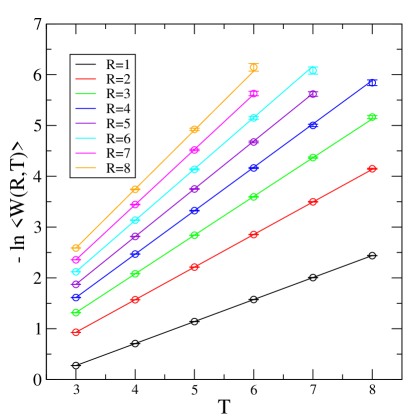
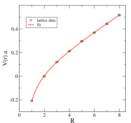
Figure 1: Linearity of the function $-\ln\;\langle W(R,T)\rangle$ in $T$ for several values of $R$ (left panel). The static quark anti-quark potential for $SU(3)$, $16^{4}$ lattice and $\beta=5.9$ (right panel).

Details concerning ${\cal P}_{3}$ can be found in [12]. Temporal links are unchanged, i.e.,

$$\Pi_{0}(x)\;=\;U_{0}(x)\;.$$ (6)

Since the projection ${\cal P}_{N}$, $N=3$ is “expensive” from a numerical point of view, we used a different method to define the cooled spatial links $\Pi_{i}(x)$, $i=1,2,3$. Let us define the action of the spatial links of a given time slice $t$ by

$$S_{(3)}(t)\;=\;\sum_{i>k,1\ldots 3}P_{ik}(x)\;,$$ (7)

where $P_{ik}(x)$ (2) is the plaquette calculated from the spatial links. In addition, we define three different embeddings of the $SU(2)$ matrix $a_{0}+i\vec{\tau}\vec{a}$, $a_{0}^{2}+\vec{a}^{2}=1$ into the group $SU(3)$, i.e.,

$$V^{(1)}\;=\;\left(\begin{matrix}1&0&0\\ 0&a_{0}+a_{3}&a_{2}-ia_{1}\\ 0&-a_{2}-ia_{1}&a_{0}-a_{3}\end{matrix}\right)\;,\;\;\;\;V^{(2)}\;=\;\left(\begin{matrix}a_{0}+a_{3}&0&a_{2}-ia_{1}\\ 0&1&0\\ -a_{2}-ia_{1}&0&a_{0}-a_{3}\end{matrix}\right)\;,$$ (8)

$$V^{(3)}\;=\;\left(\begin{matrix}a_{0}+a_{3}&a_{2}-ia_{1}&0\\ -a_{2}-ia_{1}&a_{0}-a_{3}&0\\ 0&0&1\end{matrix}\right)\;.$$ (9)

Let us now consider a particular spatial link $U_{l}(x)$. Substituting $U^{\prime}:=V^{(1)}U_{l}(x)$, we locally maximize the action $S_{(3)}$ with respect to $V^{(1)}$. Subsequently, we replace $U^{\prime}$ by $U^{\prime\prime}=V^{(2)}U^{\prime}$ and maximize with respect to $V^{(2)}$, and setting $U^{\prime\prime\prime}=V^{(3)}U^{\prime\prime}$, $V^{(3)}$ is chosen to maximize $S_{(3)}$. Finally, we define

$$\Pi_{l}(x)\;=\;V^{(3)}\;V^{(2)}\;V^{(1)}\;U_{l}(x)\;.$$ (10)

We then visit the next link on the lattice. One sweep has been performed when all spatial links of the lattice have been visited. The advantage of the present procedure is that the maximization of $S_{(3)}$ with respect to one of the $SU(2)$ subgroups can be implemented very efficiently.

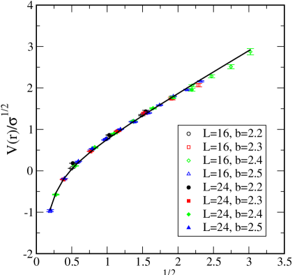
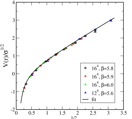
Figure 2: The static quark anti-quark potential for the $SU(2)$ gauge group (left panel) and for the case of the $SU(3)$ gauge group (right panel).

In order to achieve a good overlap with the groundstate, the above procedure for determining the links $\Pi_{l}(x)$ is applied recursively, and the Wilson loop expectation value $\langle W(R,T)\rangle$ is calculated from the configurations $\{\Pi_{\mu}(x)\}$ rather than the ensembles $\{U_{\mu}(x)\}$ . The average of $S_{(3)}$ over the time slices divided by the total number of spatial links serves as litmus paper for the overlap. It turned out that ten sweeps are enough to yield more than $0.99$ ground state overlap. Good overlap is also signaled by the quantity

$$-\ln\;\Bigl{\langle}W(R,T)\Bigr{\rangle}\;,$$ (11)

which already shows a linear behavior in $T$ for $T\geq 3$. This is illustrated for the case of a $SU(3)$ gauge group, $L^{4}=16^{4}$, and $\beta=5.9$. The final results are obtained from 100 independent measurements. The symbols in figure 1, left panel, represent the lattice data of the quantity (11); the lines are linear fits in $T$, i.e.,

$$-\ln\;\Bigl{\langle}W(R,T)\Bigr{\rangle}\;=\;\gamma T\;+\;\delta\;.$$ (12)

The coefficients $\gamma$ can be interpreted as $V(r)a$. The latter quantity is shown in figure 1, right panel (symbols). The line is a fit according to the function

$$V(r)\;a\;=\;c\;R\;-\;\frac{b}{R}\;+\;V_{0}\;,\hbox to28.45274pt{\hfill}r=R\,a\;,$$ (13)

where the parameter $c$ can interpreted as the string tension in units of the lattice spacing, i.e., $c=\sigma a^{2}$. This method for the calculation of the string tension was used, e.g., in [13]. For the present example, we find

$$\sigma\;a^{2}\,(\beta=5.9)\;=\;0.0701\;\pm\;0.0005\;,$$ (14)

which is in agreement with the value reported in the literature, i.e., $\sigma\;a^{2}\,(\beta=5.9)=0.073$  [14, 15].

2.3 The scaling relation

In order to mark a dimensionful quantity as a physically sensible one in the continuum limit $a\rightarrow 0$, it is crucial to express this quantity in units of a physical reference scale. Throughout this paper, the string tension $\sigma$ will serve this purpose.

It is time consuming but straightforward to determine the dependence of $\sigma\;a^{2}(\beta)$ on $\beta$. The results for the gauge group $SU(2)$ are summarized in table 1. Those for the case of a $SU(3)$ gauge group are shown in table 2.

L	16	24	16	24	16	24	16	24
$\beta$	2.2	2.2	2.3	2.3	2.4	2.4	2.5	2.5
$\sigma a^{2}$	0.26(2)	0.24(1)	0.146(3)	0.145(2)	0.0752(7)	0.0754(5)	0.0391(3)	0.0373(1)

Table 1: String tension $\sigma$ in units of the lattice spacing $a$ for the case of the $SU(2)$ gauge group.

L	12	16	16	16	16	16
$\beta$	5.6	5.6	5.7	5.8	5.9	6.0
$\sigma a^{2}$	0.32(1)	0.26(1)	0.169(3)	0.104(1)	0.0701(5)	0.0514(3)

Table 2: String tension $\sigma$ in units of the lattice spacing $a$ for the case of the $SU(3)$ gauge group.

These values are in good agreement with those reported, e.g., in [14].

3 The vortex texture

Concerning the criteria (i) and (ii) of the introductory section in 1, one firstly notes that the properties of the $SU(2)$ vortices extrapolate properly to the continuum limit [6] if the maximal center gauge (MCG) is used. Moreover, the MCG vortex theory correctly reproduces the de-confinement temperature [16]. The phase transition acquires a geometrical picture: is appears as a vortex de-percolation phase transition [16, 17] which already points towards a weak vortex interaction (see also [18]). Secondly, it was observed that this geometrical picture correctly reproduces the finite size scaling of the 3D Ising universality class [19]. This shows that at least for temperatures close to de-confinement, MCG vortices interact weakly.

It turns out that the non-locality induced by gauge fixing is crucial for property (i) above: it was analytically shown that if unfixed lattice configurations are projected onto vortex configurations, the complete static quark potential (including the Coulomb term) is obtained [20]. At the same time, the properties of this vortex matter strongly depend on the size of the lattice spacing. Thus, these vortices lack an interpretation in the continuum limit. In these respects the non-locality of the approach to the vortex matter is an advantage. On the other hand, however, this non-locality generically makes it difficult to access the vortex matter in practical simulations: using a variational gauge condition as, e.g., in the case of MCG [5], the definition of the vortices is ambiguous as a result of the inability to localize the global maximum of a non-linear functional. At least for small lattice sizes, the so-called Gribov ambiguity might have a significant influence on physical observables [21, 22].

Marked progress concerning the Gribov problem was made with the construction of the Laplacian gauges [23]: the non-locality of the gauge fixing is preserved while the maximization is replaced by an eigenvector problem, which can be handled by present-day algorithms. The Laplacian version of the MCG was firstly proposed for a $SU(2)$ gauge group in [24] and generalized to the $SU(3)$ case in [25]. A further improvement was reported in [29]. Vortex matter of the Laplacian center gauge (LCG) is unambiguously defined and recovers the asymptotic string tension for both gauge groups, $SU(2)$ and $SU(3)$. In the case of a $SU(2)$ gauge theory, it was, however, observed that the LCG vortices are produced in large abundance, implying that they lie dense (nevertheless in a controlled way) in the continuum limit [7]. This indicates a rather strong interaction of LCG vortices, which might render it difficult to mimic LCG vortex matter in a low-energy effective model.

The present section briefly reviews details of the center gauge fixing procedures and the vortex projection techniques with an emphasis on the case of $SU(3)$.

3.1 The ideal center vortex cluster

In order to reveal degrees of freedom which are relevant for confinement, we are looking for configurations $\{Z_{\mu}(x)\}$, $Z_{\mu}(x)\in Z_{N}$ which best represent the full link configurations $\{U_{\mu}(x)\}$, $U_{\mu}(x)\in SU(N)$. Thereby, $Z_{N}$ represents the center of the group $SU(N)$, i.e.,

$$Z_{\mu}(x)\;=\;\exp\Bigl{\{}i\frac{2\pi}{N}\;m\Bigr{\}}\;,\hbox to28.45274pt{\hfill}-\frac{N}{2}<m\leq\frac{N}{2}\;,$$ (15)

where $m$ is an integer. There is an optimal choice of the gauge for which the overlap of the center configurations with the full ones is maximal. Let us denote the gauge transformed links by

$$U^{\Omega}_{\mu}(x)\;=\;\Omega(x)\;U_{\mu}(x)\;\Omega^{\dagger}(x+\mu)\;,\hbox to28.45274pt{\hfill}\Omega(x)\in SU(N)\;.$$ (16)

In oder to obtain the ideal center configurations, we minimize the functional

$$\sum_{x,\mu}\Bigl{[}U^{\Omega}_{\mu}(x)\;-\;Z_{\mu}(x)\Bigr{]}^{\dagger}\;\Bigl{[}U^{\Omega}_{\mu}(x)\;-\;Z_{\mu}(x)\Bigr{]}\;\;\stackrel{{\scriptstyle\Omega,Z_{\mu}}}{{\longrightarrow}}\;\;\mathrm{min}$$ (17)

with respect to $\Omega(x)$ and $Z_{\mu}(x)$. The selection of $\Omega(x)$ implies the choice of a gauge. We will call this gauge ideal center gauge (ICG) throughout this paper. The condition (17) directly implies that the overlap, i.e.,

$$R\;=\;\frac{1}{N_{l}}\;\sum_{x,\mu}\;\Re\;\frac{1}{N}\;\text{tr}\Bigl{(}U^{\Omega}_{\mu}(x)\;Z^{\dagger}_{\mu}(x)\Bigr{)}\;,$$ (18)

is maximized. $N_{l}$ is the number of links of the lattice, and $-1\leq R\leq 1$. $R=1$ means that the link configuration $\{U_{\mu}(x)\}$ can be entirely expressed in terms of center elements after a suitable gauge has been chosen.

The maximization of $R$ with respect to the center elements $Z_{\mu}(x)$ can be performed locally: with

$$\frac{1}{N}\;\text{tr}U^{\Omega}_{\mu}(x)\;=\;u_{l}\,\exp\{i\varphi^{l}\},\hbox to28.45274pt{\hfill}Z_{\mu}(x)\;=\;\exp\{i\varphi^{l}_{m}\}\;,\hbox to28.45274pt{\hfill}\varphi_{m}=\frac{2\pi}{N}\;m\;,$$ (19)

where $l=\{x,\mu\}$ specifies the link, one finds

$$R\;=\;\frac{1}{N_{l}}\;\sum_{l}\;u_{l}\;\cos\Bigl{(}\varphi^{l}-\varphi^{l}_{m}\Bigr{)}\;.$$

The optimal choice is obtained by choosing $m$ (19) in such a way that $\varphi^{l}_{m}$ is closest to $\varphi^{l}$. This mapping

$$SU(N)\rightarrow Z_{N}:\;\;U^{\Omega}_{\mu}(x)\rightarrow Z_{\mu}(x)\;=\;{\cal Z}\Bigl{(}U^{\Omega}_{\mu}(x)\Bigr{)}$$ (20)

is called center projection. Inserting $Z_{\mu}(x)$ from (20) into (18), the overlap $R$ must then be maximized with respect to the gauge transformations, i.e., $\Omega(x)$.

3.2 Center gauges

Since the mapping (20) by no means depends smoothly on $\Omega(x)$, an iteration over-relaxation algorithm which iteratively determines $Z_{\mu}(x)$ and $\Omega(x)$ from (18) can hardly work. State of the art would be to determine the desired quantities $Z_{\mu}(x)$, $\Omega(x)$ by the technique of “simulated annealing”. However in this case, determining, e.g., $\Omega(x)$ to the precision which is needed for the vortex analysis is extremely costly from a numerical point of view. This approach is beyond the scope of the present paper and is left to future investigations.

In order to make the gauge fixing efficient by means of iteration over-relaxation, we assume that in the optimal case, $1/N\;\text{tr}U^{\Omega}_{\mu}(x)$ comes close to a center element. In this case, we relax the condition which constrains ${\cal Z}(U^{\Omega}_{\mu}(x))$ in (20) to a center element. There are two possibilities for doing this:

$${\cal Z}\Bigl{(}U^{\Omega}_{\mu}(x)\Bigr{)} \propto \Bigl{(}\text{tr}U^{\Omega}_{\mu}(x)\Bigr{)}^{\dagger}\;,$$ (21)

$${\cal Z}\Bigl{(}U^{\Omega}_{\mu}(x)\Bigr{)} \propto \Bigl{(}\text{tr}U^{\Omega}_{\mu}(x)\Bigl{)}^{2}\;.$$ (22)

Hence, we find the gauge conditions

$$R_{mes} = \frac{1}{N_{l}}\;\sum_{x,\mu}\;\Bigl{[}\frac{1}{N}\;\text{tr}\Bigl{(}U^{\Omega}_{\mu}(x)\Bigr{)}\;\Bigr{]}\;\Bigl{[}\frac{1}{N}\;\text{tr}\Bigl{(}U^{\Omega}_{\mu}(x)\Bigr{)}\;\Bigr{]}^{\dagger}\;,$$ (23)

$$R_{bar} = \frac{1}{N_{l}}\;\sum_{x,\mu}\;\Re\;\Bigl{[}\frac{1}{N}\;\text{tr}\Bigl{(}U^{\Omega}_{\mu}(x)\Bigr{)}\;\Bigr{]}^{3}\;;$$ (24)

both have been advertised in the literature [27]. It is not clear at the beginning which of the above possibilities yields the larger overlap (18). It might turn out that even a background-field-dependent admixture of both possibilities (21,22) is best for the present purposes. Since the algorithm for the so-called “mesonic” gauge (23) was already studied in the literature to a large extent [27, 28], we will employ the gauge condition $R_{mes}\rightarrow max$ for the determination of $\Omega(x)$ and perform subsequent center projection along the lines outlined in the previous subsection.

Even once we have agreed on one of the suboptimal gauge conditions (23,24), there is still the problem of the Gribov ambiguities: since the overlap $R$ is a non-linear functional on $\Omega(x)$, detecting the global maximum of $R$ is practically impossible for reasonable lattice sizes. The choice of the local maximum of $R$ which is implicitly defined by the algorithm determines the gauge. Although the physics extracted in the latter gauge can be highly relevant for confinement, the definition of gauge by the numerical procedure is unsatisfactory. The Gribov problem can be solved by adopting the Laplacian version [23, 24, 25, 30]of the maximal center gauges. A detailed study of these gauges and the corresponding vortex matter can be found for the case of $SU(2)$ in [7] and for the case of $SU(3)$ in [25]. Here, we will briefly outline the procedure for the case of $SU(3)$ and refer the reader to reference [25] for details.

The generators $t^{a}$ of the $SU(N)$ algebra satisfy the equation

$$t^{a}_{ki}\;t^{a}_{lm}\;=\;\frac{1}{2}\Bigl{(}\delta_{il}\;\delta_{mk}\;-\;\frac{1}{N}\delta_{lm}\;\delta_{mk}\Bigr{)}\;,\hbox to28.45274pt{\hfill}\text{tr}\;t^{a}t^{b}\;=\;\frac{1}{2}\delta^{ab}\;.$$ (25)

With the help of this identity, the “mesonic” functional $R_{mes}$ (23) can be written as

$$R_{mes}\;=\;\frac{1}{N_{l}}\;\sum_{x,\mu}\;\frac{1}{N^{2}}\;\Bigl{[}\text{tr}\;O^{T}(x)\;R_{\mu}(x)\;O(x+\mu)\;+\;1\Bigl{]}\;,$$ (26)

where the adjoint matrices are defined by

$$O^{ab}(x)\;=\;2\,\text{tr}\Bigl{\{}t^{a}\;\Omega(x)\;t^{b}\;\Omega^{\dagger}(x)\Bigr{\}}\;,\hbox to28.45274pt{\hfill}R_{\mu}^{ab}(x)\;=\;2\,\text{tr}\Bigl{\{}t^{a}\;U_{\mu}(x)\;t^{b}\;U_{\mu}^{\dagger}(x)\Bigr{\}}\;.$$ (27)

Equation (26) can be written as

$$N^{2}\;R_{mes}\;=\;\frac{1}{N_{l}}\text{Tr}\;{\cal O}^{T}\;{\cal R}\;{\cal O}\;+\;1\;,$$ (28)

where we have introduced, e.g., the vector ${\cal O}$ of the combined coordinate and color space, $\{O^{ab}(x)\}\rightarrow{\cal O}$. Up to a term proportional to the unit matrix, ${\cal R}$ is the adjoint Laplacian operator, i.e.,

$${\cal R}^{ab}_{xy}\;=\;\frac{1}{2}\;\sum_{\mu}\bigl{[}R_{\mu}^{ab}(x)\;\delta_{y,x+\mu}\;+\;R_{\mu}^{ba}(x-\mu)\;\delta_{y,x-\mu}\;\Bigr{]}\;.$$ (29)

Note that the vector ${\cal O}$ is subjected to the constraints that the set of vectors $n^{a}$ with $O_{ab}(x)=\{n^{1}(x),\,n^{2}(x),\,n^{3}(x)\}_{ab}$ is orthonormal. At the heart of Laplacian center gauge fixing, one relaxes these constraints and seeks the $N-1$ largest eigenvalues of the super-matrix ${\cal R}$. These tasks can be unambiguously performed with present-day algorithmic tools. From the corresponding eigenvectors, the adjoint gauge transformations $O^{ab}(x)$ are reconstructed at each site with the help of Gram-Schmidt orthogonalization. Abelian monopoles and vortices appear as defects in the latter step of reconstructing the gauge transformation. Technical details of this gauge fixing are presented in [25]. Finally, we point out that the Laplacian gauge also seeks to maximize the “mesonic” gauge condition. However, the re-orthogonalization of the eigenvectors implies that the values for the overlap $R$ (18) are significantly smaller than that achieved by maximizing $R_{mes}$ (23) with the help of an iteration over-relaxation procedure.

3.3 Identifying vortex matter

In order to reveal the vortex matter of $Z_{N}$ gauge theory, we define

$$v(p)\;:=\;\prod_{l\in p}Z_{l}\;,\;\;l=\{x,\mu\}\;,\;\;\;v(p)\in Z_{N}\;,$$ (30)

where $p=(x,\mu<\nu)$ defines an elementary plaquette on the lattice. One says that a vortex of center charge $z$ pierces the plaquette $p$ if

$$v(p)\;=\;z\;,\hbox to28.45274pt{\hfill}z\;=\;\exp\Bigl{\{}i\frac{2\pi}{N}\;\varphi\Bigr{\}}\;,$$ (31)

where $-\frac{N}{2}<\varphi(p)\equiv\varphi_{\mu\nu}(x)\leq\frac{N}{2}$ is called the center flux. For $SU(N\geq 3)$, one defines the conserved $Z_{N}$ monopole current by

$$m_{\mu}(x)\;=\;\frac{1}{N}\;\epsilon_{\mu\nu\alpha\beta}\;\Delta_{\nu}\;\varphi_{\alpha\beta}(x)\;,\hbox to28.45274pt{\hfill}\Delta_{\mu}\;m_{\mu}(x)\;=\;0\,,$$ (32)

where

$$\Delta_{\mu}\;\Phi(x)\;:=\;\Phi(x+\mu)\;-\Phi(x)\;.$$

In order to reveal the span of the monopole charge $m_{4}$, we consider an elementary, spatial hypercube $c=(x,\alpha<\beta<\gamma)$. One easily verifies, using the Abelian nature of the group $Z_{N}$, that

$$1\;=\;\prod_{p\in c}D\Bigl{[}v(p)\Bigr{]}\;=\;\exp\Bigl{\{}i\frac{2\pi}{N}\;\epsilon_{ikm}\Delta_{i}\varphi_{km}(x)\;\Bigr{\}}\;,$$ (33)

where the sum over $i,k,m$ runs from $1\ldots 3$, and $D[v(p)]=v^{\dagger}(p)$ if the normal vector of the plaquette is anti-aligned with the normal vector of the relevant surface element of $c$, and $D[v(p)]=v(p)$ otherwise. Hence, the monopole charge comes in integers, i.e.,

$$m_{4}\;=\;\frac{1}{N}\;\epsilon_{ikm}\Delta_{i}\varphi_{km}(x)\;=\;k\;,\hbox to28.45274pt{\hfill}k:\,\mathrm{integer}\;.$$ (34)

Finally, we point out that there are no center monopoles in the case of a $SU(2)$ gauge group, i.e., $m_{\mu}(x)\equiv 0$.

It is convenient for model building to define the vortex matter on the dual lattice, where the link $l$, the plaquette $p$ and the cube $c$ is mapped onto

$$l\;\longrightarrow\;c^{\ast}\;,\hbox to28.45274pt{\hfill}p\;\longrightarrow\;p^{\ast}\;,\hbox to28.45274pt{\hfill}c\;\longrightarrow\;l^{\ast}\;.$$ (35)

The vortex field of the dual lattice is defined via the identification

$$\bar{v}(p^{\ast})\;=\;v(p)\;,\hbox to56.9055pt{\hfill for \hfill}p\;\longrightarrow\;p^{\ast}\;.$$ (36)

The identity (33) can be transformed into an identity for dual fields only:

$$1\;=\;\prod_{p^{\ast}\ni l^{\ast}}\bar{v}(p^{\ast})\,.$$ (37)

The latter equation implies that the vortices either from closed world sheets on the dual lattice or, for $SU(N\geq 3)$ only, multiples of $N$ vortex world sheets merge at a closed monopole trajectory.

4 Dominance of the static quark potential

Preliminary evidence that the MCG vortex matter recovers the string tension of pure $SU(3)$ gauge theory was presented in [27]. The so-called indirect center gauge, i.e., maximal Abelian gauge fixing with a subsequent fixing of the center gauge, was investigated in [13]. There it was observed that the string tension obtained from Abelian monopole configurations as well as from $Z_{3}$ vortex ensembles is significantly smaller than the string tension of complete $SU(3)$ gauge theory. On the other hand, it is interesting to note that the $SU(3)$ string tension is recovered to full extent in the case of the LCG [25].

Here, we will see that the MCG vortices act like the vortices defined in the indirect center gauge: roughly 62% of the full string tension is found. We will therefore find that the MCG vortex ensembles genuinely differ from those of the LCG.

4.1 The case of a $SU(2)$ gauge group revisited

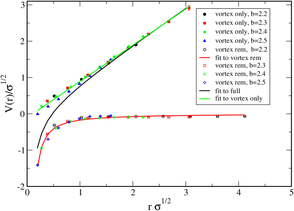
Figure 3: The static quark anti-quark potential for the $SU(2)$ gauge group: full ensembles, vortex projected ensembles, and ensembles where the vortices have been removed (see (39)). Lattice size: $24^{4}$.

In order to contrast the findings concerning the $SU(3)$ gauge group, which will be presented below, with the findings for the case of $SU(2)$, we briefly discuss our numerical results for the latter case in this subsection.

The maximal center gauge (23) is implemented by using the iteration over-relaxation procedure which is described in detail in [5]. This procedure defines the gauge. The corresponding vortex degrees of freedom are defined by the projection (20), which becomes in the present case:

$$SU(2)\rightarrow Z_{2}:\;\;U^{\Omega}_{\mu}(x)\rightarrow Z_{\mu}(x)\;=\;\mathrm{sign}\;\text{tr}\;U^{\Omega}_{\mu}(x)\;.$$ (38)

It turns out that this procedure produces vortex configurations with sensible properties in the continuum limit [6] and with a close relation to the physics of confinement [5, 4, 16, 17]. So far, vortex matter with “best” properties in the continuum limit seems to obtained with a ’preconditioning’ by performing the Laplacian center gauge (see subsection 3.2) and subsequent maximal center gauge fixing [7, 29]. This approach also alleviates the Gribov problem, but its implementation is numerically “expensive”.

In order to reveal the relevance of the vortex texture for the physics of confinement, one firstly calculates the static quark potential from the vortex configurations. Secondly, one defines a toy Yang-Mills theory by

$$U^{\prime}_{\mu}(x)\;=\;Z^{\dagger}_{\mu}(x)\;U^{\Omega}_{\mu}(x)\;,$$ (39)

where the vortex texture has been removed “by hand” from the lattice ensembles. It was found [4, 5] that the vortex configurations reproduce the linear part of the potential to a large extent. In addition, the potential evaluated from the modified configurations $\{U^{\prime}_{\mu}(x)\}$ has lost its linear rise and shows a Coulomb type of behavior. Both observations are summarized by the term ’center dominance of the potential’.

Figure 3 illustrates these observations using our lattice results. Only data which were obtained on a $24^{4}$ lattice are shown. The number of independent configurations employed for the calculation of expectation values is listed in table 3.

$\beta$	2.2	2.3	2.4	2.5
$\#$	75	75	35	55

Table 3: Number of independent $SU(2)$ configurations used for the calculation of the static potential (see figure 3).

The full configurations $\{U_{\mu}(x)\}$ as well as the configurations $\{U^{\prime}_{\mu}(x)\}$ from which the vortices have been removed “by hand” are subject to the overlap enhancement described in subsection 2.2. The $Z_{2}$ vortex configurations already possess good overlap with the ground state, and no enhancement is used in this case. The line which fits the “vortex only” data in figure 3 corresponds to a string tension of 97.7% of the full string tension. we stress that these findings have been obtained with the most naive version of the maximal center gauge (described in [5]).

Finally, we point out that the quality of dominance is affected by the choice of gauge, i.e., the Gribov copy [21], and that the Gribov effect is influenced by the lattice volume [22].

4.2 Vortex-limited Wilson loops: $SU(3)$ gauge group

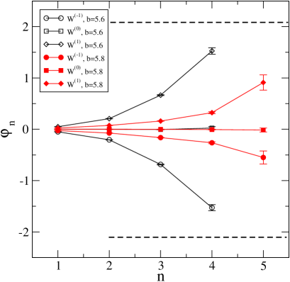
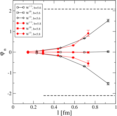
Figure 4: The angle $\varphi^{(m)}$ of the Wilson loop expectation values (43) as a function of the Wilson loop size $n$ (left panel) and as a function of the size in physical units (right panel).

Let $W_{n}[U_{\mu}]$ denote a $n\times n$ planar Wilson loop calculated within the particular configuration $U_{\mu}(x)$. The same object is evaluated with the $Z_{3}$ configurations obtained from center projection (20) after direct maximal center gauge fixing using the “mesonic” gauge condition (23). The result is called $W_{n}[Z_{\mu}]$. Since $W_{n}[Z_{\mu}]\in Z_{3}$, the latter Wilson loop can be characterized by the number $m\in\{-1,0,1\}$, i.e.,

$$W_{n}[Z_{\mu}]\;=\;\exp\Bigl{\{}i\frac{2\pi}{3}\;m\Bigr{\}}\;.$$ (40)

The expectation value of the Wilson loop,

$$W_{n}\;=\;\Bigl{\langle}W_{n}[U_{\mu}]\Bigr{\rangle}\;,$$ (41)

is obtained by averaging over the ensembles $\{U_{\mu}(x)\}$. In addition, we can define expectation values

$$W^{(m)}_{n}\;=\;\Bigl{\langle}W_{n}[U_{\mu}]\Bigr{\rangle}_{m}\;,$$ (42)

where only loops $W_{n}[U_{\mu}]$ are taken into account; the corresponding quantity $W_{n}[Z_{\mu}]$ belongs to the sector $m$. Decomposing

$$W^{(m)}_{n}\;=\;|W^{(m)}_{n}|\;\exp\Bigl{\{}i\varphi^{(m)}_{n}\Bigr{\}},$$ (43)

one expects that for large loops

$$\lim_{n\to\infty}\varphi^{(m)}_{n}\;=\;\frac{2\pi}{3}\;m\;,$$ (44)

if center vortices dominate the Wilson loop expectation value. The latter relation can be checked by lattice simulations. The quantity $\varphi^{(m)}_{n}$ is shown for $\beta=5.6$ ($227$ independent measurements) and for $\beta=5.8$ ($160$ independent measurements) in figure 4 as a function of $n$ (left panel). It seems that the relation (44) is indeed satisfied for large $n$. If we plot the angle $\varphi^{(m)}_{n}$ as a function of the physical size of the Wilson loop, i.e., $l=n\,a(\beta)$, we observe that the data for $\beta=5.6$ and for $\beta=5.8$, respectively, roughly fall on top of the same curve (right panel).

Let us interpret these findings from a random vortex model point of view. Following [26], we assume that center vortex intersection points possess a finite correlation length $L_{c}$. Thus dividing the minimal area $A$ of the planar Wilson loop into squares of size ${\cal A}>L_{c}^{2}$, the center fluxes $\varphi\in\{-1,0,1\}$ through different squares are essentially uncorrelated. Let $\widetilde{\rho}(m,{\cal A})$ denote the probability of finding center flux $m$ through the area ${\cal A}$; we define the “mesoscopic” vortex density by

$$\rho_{mes}\;:=\;\widetilde{\rho}(m,{\cal A})\;/\;{\cal A}\;,\hbox to28.45274pt{\hfill}A\;=\;n^{2}\,a^{2}(\beta)\;.$$ (45)

Assuming vortex dominance, we might approximate

$$W_{n}\;=\;\Bigl{\langle}W_{n}[U_{\mu}]\Bigr{\rangle}\;\approx\;\Bigl{\langle}W_{n}[Z_{\mu}]\Bigr{\rangle}\;.$$ (46)

Using the fact that center fluxes are uncorrelated by construction, one obtains

$$W_{n}\;\approx\;\Bigl{\langle}W_{n}[Z_{\mu}]\Bigr{\rangle}\;=\;\langle Z\rangle^{A/{\cal A}}\,,$$ (47)

where $\langle Z\rangle$ the average flux through the area ${\cal A}$ is

$$\langle Z\rangle\;=\;\sum_{m=-1..1}\widetilde{\rho}(m,{\cal A})\;\;\exp\Bigl{\{}i\frac{2\pi}{3}\;m\Bigr{\}}\;.$$ (48)

Hence, the string tension in the center flux approximation is given by

$$\sigma_{cf}\;=\;-\frac{1}{\cal A}\;\ln\,\Bigl{[}\sum_{m=-1..1}\widetilde{\rho}(m,{\cal A})\;\;\exp\{i\frac{2\pi}{3}\;m\}\Bigr{]}\;=\;-\frac{1}{\cal A}\;\ln\,\,\Bigl{(}1\;-\;3\;\widetilde{\rho}\Bigr{)}\;,$$ (49)

where we have assumed that the center symmetry $m\rightarrow-m$ is not spontaneously broken, i.e.,

$$\widetilde{\rho}(1,{\cal A})\;=\;\widetilde{\rho}(-1,{\cal A})\;=:\;\widetilde{\rho}({\cal A})\;,\hbox to56.9055pt{\hfill and \hfill}\sum_{m=-1}^{1}\widetilde{\rho}(m,{\cal A})\;=\;1\;.$$ (50)

A particular case is obtained by considering that the vortices which are defined at the level of the elementary plaquette are uncorrelated (naive random vortex model). In this case, one finds

$$\widetilde{\rho}({\cal A}=a^{2})\;=\;\frac{\rho}{2}\;a^{2}\;\ll\;1\,,\hbox to85.35826pt{\hfill and thus \hfill}\sigma_{cf}\;\approx\;\frac{3}{2}\;\rho\;.$$ (51)

Thereby, $\rho$ is the “microscopic” vortex density, i.e., $\rho a^{2}$ is the probability of finding a non-trivial center flux through a given plaquette (no matter whether $m=-1$ or $m=1$).

Using the numerical data above, it is possible to estimate the center flux correlation length. Let us define the “half-width” $L_{1/2}$ by the length of the Wilson loop at which

$$\varphi^{(1)}(l=L_{1/2})\;=\;\frac{\pi}{3}\,.$$ (52)

The findings (see figure 4, right panel) suggest that

$$L_{c}\;\geq\;L_{1/2}\;\approx\;0.8\;\mathrm{fm}\,,$$ (53)

where we have used a string tension of $\sigma=(440\;\mathrm{MeV})^{2}$ as a reference scale. Finally, let us check whether the naive random vortex model of uncorrelated vortex plaquettes is realistic. For this to be the case, the relation

$$\frac{\rho}{2}\;{\cal A}\;\approx\;\frac{\rho}{2}\;L^{2}_{1/2}\;\approx\;\frac{\sigma_{cf}}{3}\;L^{2}_{1/2}\approx\;\frac{\sigma}{3}\;L^{2}_{1/2}\;\ll\;1$$ (54)

must hold. However, one finds, using (53),

$$\frac{\sigma}{3}\;L^{2}_{1/2}\;\approx\;1.03\;,$$ (55)

implying that the naive random vortex model seems not always to be justified.

4.3 The “mesonic” center gauge for $SU(3)$

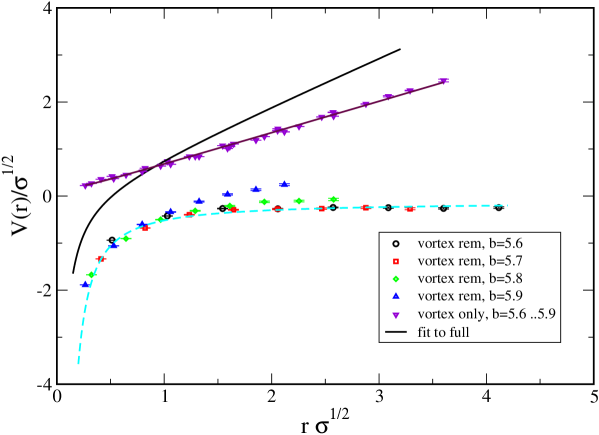
Figure 5: The static quark anti-quark potential for the $SU(3)$ gauge group: full ensembles, vortex projected ensembles, and ensembles where the vortices have been removed (see (39)). Lattice size: $16^{4}$.

In a first step, the “mesonic” gauge condition (23) is installed with the help of the iteration over-relaxation algorithm described in detail in [27, 28]. The $Z_{3}$ link elements $Z_{\mu}(x)$ are defined by center projection (20). As in the case of $SU(2)$, we will compare the static quark potential obtained from full link configurations (see section 2) with the one calculated with link ensembles $\{Z_{\mu}(x)\}$. In addition, the toy model is defined by configurations $\{U^{\prime}_{\mu}(x)\}$ (39) from which the vortices have been removed “by hand”. From the results of the previous subsection, we expect that the string tension is lost in the latter case. Our numerical findings using $100$ independent measurements are summarized in figure 5.

We find that the potential calculated from vortex configurations scales towards the continuum limit, i.e., the data obtained from different $\beta$ values fall on top of the same curve if the $V(r)$ and $r$ are expressed in physical units. In addition, one observes “precocious” linearity: the potential is linear even at small distances as is the case for a $SU(2)$ gauge group. In contrast to the case of an $SU(2)$ gauge group, the center projected string tension is only 62% of the full string tension. The value of string tension (in lattice units) after center projection is in agreement with the finding in [27] for a $12^{4}$ lattice and $\beta=5.6$. In the latter article, however, the quoted value of the full string tension is underestimated. Using reliable values, the ratio of projected and full string tension is in agreement with the findings reported here.

On the other hand, removing the vortices (see (39)) produces configurations which are compatible with a vanishing string tension. There is a subtlety for obtaining this result: the lattice volume must be large enough. It appears that the lattice size of $16^{4}$ seems to be too small for $\beta$ as big as $6.0$.

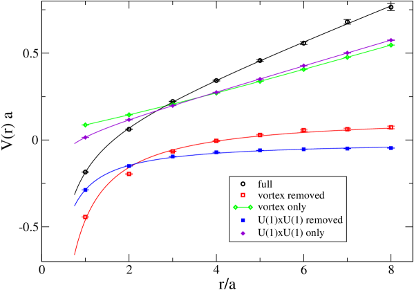
Figure 6: The static quark anti-quark potential for the $SU(3)$ gauge group: full ensembles, vortex projected ensembles, and ensembles where the vortices have been removed (see (39)). Same with $U(1)\times U(1)$ projection. Lattice size: $16^{4}$, $\beta=5.8$.

Since a removal of the vortices results in a loss of the string tension, even if the vortices only amount to 62% of the full one, the question arises as to whether additional degrees of freedom which reside in the $U(1)\times U(1)$ Abelian subgroup are responsible for the 38% string tension completing the vortex contribution. Candidates for such degrees of freedom are color magnetic monopoles. To answer this question, we implemented the “mesonic” gauge condition (23) and subsequently projected the gauged configurations onto Abelian ones:

$$U^{\Omega}_{\mu}(x)\longrightarrow V_{\mu}(x)\;,\hbox to28.45274pt{\hfill}V_{\mu}(x)\in U(1)\times U(1)\;.$$ (56)

For these purposes, the off-diagonal elements of $U^{\Omega}_{\mu}(x)$ were dropped, i.e.,

$$U^{\Omega}_{\mu}(x)\longrightarrow\bar{U}^{\Omega}_{\mu}(x):=\mathrm{diag}\Bigl{(}U^{\Omega}_{\mu}(x)\Bigr{)}\;,$$ (57)

and $V_{\mu}(x)$ is given by the $SU(3)$ element which is “closest” to $\bar{U}^{\Omega}_{\mu}(x)$ (see discussion in subsection 2.2). One verifies that indeed $V_{\mu}(x)\in U(1)\times U(1)$. In addition, we investigated ensembles $\{U^{ABR}_{\mu}(x)\}$ which are complementary to the $U(1)\times U(1)$ configurations:

$$U^{ABR}_{\mu}(x)\;=\;V^{\dagger}_{\mu}(x)\;U^{\Omega}_{\mu}(x)\;.$$ (58)

Our numerical findings for a $16^{4}$ lattice at $\beta=5.8$ are shown in figure 6. we find that the string tension calculated from $U(1)\times U(1)$ configurations is marginally larger than the string tension from vortex projected configurations. As expected, configurations $U^{ABR}_{\mu}(x)$ from which the Abelian subgroup was removed do not support confinement.

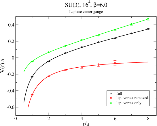
Figure 7: The static quark anti-quark potentials for the $SU(3)$ gauge group using the Laplacian center gauge: full ensembles, vortex projected ensembles, and ensembles where the vortices have been removed (see (39)). Lattice size: $16^{4}$, $\beta=6.0$.

These results are compared with those in [13]: there, versions of the so-called Maximal Abelian Gauge were investigated. These gauges are most suitable for a projection of configurations $U^{\Omega}_{\mu}(x)$ onto the Abelian subgroup $U(1)\times U(1)$. Also in these cases, the string tension extracted from $U(1)\times U(1)$ configurations is substantially smaller than the full string tension.

4.4 Laplacian center gauge

The previous subsection showed that the “mesonic gauge” (23) produces vortex matter which recovers only 62% of the full string tension. The question is whether $Z_{3}$ matter is able to give the full result for the string tension at all. The answer was already given in [25]: vortex matter which is defined by the Laplacian gauge condition (see subsection 3.2) reproduces the linear rise of the static quark potential in the continuum limit. Here, we briefly report our findings. We investigated the somewhat extreme case of a small physical volume, i.e., $16^{4}$ lattice, $\beta=6.0$. The last subsection showed that for this size the removal of the vortices defined by the “mesonic gauge” hardly makes the string tension vanish. The result of $50$ independent measurements is shown in figure 7. The potentials of this figure were fitted by the function

$$V(r)\;a^{2}\;=\;\sigma\;a^{2}\;n\;\;-\;\;\frac{\alpha}{n}\;,\hbox to28.45274pt{\hfill}r=na\,.$$ (59)

In either case we find

$$\mathrm{vortex\;only}\; : \;\sigma a^{2}\;=\;0.061\;\hbox to28.45274pt{\hfill}\alpha\;=\;0.096\;,$$

$$\mathrm{vortex\;removed}\; : \;\sigma a^{2}\;=\;0.0\phantom{61}\;\hbox to28.45274pt{\hfill}\alpha\;=\;0.43\;,$$

$$\mathrm{full}\; : \;\sigma a^{2}\;=\;0.051\;\hbox to28.45274pt{\hfill}\alpha\;=\;0.25\;.$$

A small Coulomb part survives the projection onto vortices. One also observes that the potential obtained from configurations from which the Laplacian vortices have been removed is perfectly fitted by a Coulomb law. The string tension from vortex configurations is a bit higher than the full string tension. This is probably due to the small physical size of the lattice: Coulomb contributions are dominant and are represented by the vortex matter as string tension to some extent.

It turns out [7, 29] in the case of the $SU(2)$ gauge group that preconditioning with the Laplace center gauge and subsequent implementation of the “mesonic” gauge by iteration over-relaxation strongly reduces the influence of the Gribov copies. Center projection of these ensembles yields high-quality vortex matter the properties of which nicely extrapolates to the continuum limit. We have checked that repeating this approach for the $SU(3)$ case produces vortex matter where the corresponding string tension again only reaches 62% of the full string tension.

5 Properties of $SU(3)$ vortex matter

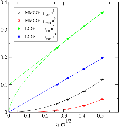
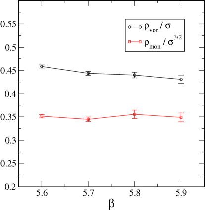
Figure 8: The continuum limit of the vortex- and the $Z_{3}$ monopole density for the “mesonic” gauge and the Laplacian gauge (left panel). The vortex- and the $Z_{3}$ monopole density in physical units for the “mesonic gauge” (right panel).

In this section, we will investigate which definition of the vortex matter (MCG or LCG) admits an interpretation of the vortices as physical degrees of freedom. To this aim, the continuum limit $a\rightarrow 0$ of the planar vortex density $\rho_{\mathrm{vor}}$ (i.e., the “microscopic” vortex density of subsection 4.2) and the density $\rho_{\mathrm{mon}}$ of $Z_{3}$ monopoles are investigated.

The vortex density $\rho_{\mathrm{vor}}$ can be extracted from the $Z_{3}$ ensembles $\{Z_{\mu}(x)\}$ as follows: we say that a $Z_{3}$ plaquette,

$$v(p)\;:=\;\prod_{l\in p}Z_{l}\;,\;\;l=\{x,\mu\}\;,\;\;\;v(p)\in Z_{3}\;,$$ (60)

carries a non-trivial center flux if

$$v(p)\;=\;z\;,\hbox to28.45274pt{\hfill}z\;=\;\exp\Bigl{\{}i\frac{2\pi}{3}\;\varphi\Bigr{\}}$$ (61)

and $\varphi=-1$ or $\varphi=1$. If ${\cal P}_{\beta}$ denote the probability that a particular plaquette of the lattice carries a non-trivial center charge, the vortex density is defined by

$$\rho_{\mathrm{vor}}\;a^{2}(\beta)\;=\;{\cal P}_{\beta}\;.$$ (62)

As outlined in subsection 3.3, the $Z_{3}$ monopole world lines are associated with dual links whose corresponding monopole current $m_{\mu}(x)$ (32) is non-zero. Alternatively, 3d hypercubes from which non-trivial center flux emerges are said to contain a center monopole. Given that ${\cal Q}_{\beta}$ is the probability that a particular hypercube contains a center monopole, the monopole density is obtained from

$$\rho_{\mathrm{mon}}\;a^{3}(\beta)\;=\;{\cal Q}_{\beta}\;.$$ (63)

Both quantities characterize the vortex matter. In order to interpret the vortices as sensible degrees of freedom in the continuum limit $a\rightarrow 0$, the quantities must obey

$$\lim_{\beta\to\infty}\rho_{\mathrm{vor}}\;=\;\mathrm{constant}\;,\hbox to28.45274pt{\hfill}\lim_{\beta\to\infty}\rho_{\mathrm{mon}}\;=\;\mathrm{constant}\;.$$ (64)

Our numerical findings are summarized in figure 8. Figure 8, left panel shows the densities $\rho_{\mathrm{vor}}$ and $\rho_{\mathrm{mon}}$ in units of the lattice spacing as a function of $a\;\sqrt{\sigma}$. Simulations were performed for $\beta=5.6$, $5.7$, $5.8$, $5.9$. The corresponding size of the lattice spacing can be found in table 2.

Let us firstly focus on vortex matter obtained after implementing the “mesonic” gauge condition (23). There, the data are perfectly fitted by

$$\rho_{\mathrm{vor}}\;a^{2}(\beta) \approx 0.45\;\Bigl{(}a\;\sqrt{\sigma}\Bigr{)}^{2}\;,$$ (65)

$$\rho_{\mathrm{mon}}\;a^{3}(\beta) \approx 0.35\;\Bigl{(}a\;\sqrt{\sigma}\Bigr{)}^{3}\;.$$ (66)

These findings suggest that the planar areal vortex density as well as the $Z_{3}$ monopole density properly extrapolate to the continuum limit (see figure 8, right panel). The same result for the vortex density was found for the case of a $SU(2)$ gauge group [6, 5]. In a naive random vortex model, one expects that the string tension is given by (see (51))

$$\sigma_{cf}\;\approx\;\frac{3}{2}\;\rho_{\mathrm{vor}}\;\approx\;0.67\;\sigma\;.$$ (67)

We point out that the naive string tension $\sigma_{cf}$ roughly agrees with the string tension measured from center projected configurations (see subsection 4.3), i.e.,

$$\sigma_{Z3}\;\approx\;0.62\;\sigma\;.$$

This indicates that the intersection points of the “mesonic” center vortex clusters do not contain significant long-range correlations. Using $\sqrt{\sigma}=440\,$MeV as a reference scale, one finds for the SU(3) case

$$\rho_{\mathrm{vor}}\;\approx\;2.2\;\frac{1}{\mathrm{fm}^{2}}\;,\hbox to28.45274pt{\hfill}\rho_{\mathrm{mon}}\;\approx\;3.7\;\frac{1}{\mathrm{fm}^{3}}\;,\hbox to28.45274pt{\hfill}\frac{\rho_{\mathrm{mon}}}{\rho^{3/2}_{\mathrm{vor}}}\;\approx\;1.16\;.$$ (68)

The latter quantity might be of interest for the construction of $Z_{3}$ random vortex models.

As already noticed for a $SU(2)$ gauge group [7], the situation drastically changes for the Laplacian center gauge. The vortex and monopole densities (times the canonical powers of the lattice spacing) scale linearly with the lattice spacing. Two fits represent the areal vortex density almost equally well:

$$\rho_{\mathrm{vor}}\;a^{2}(\beta)\;\approx\;0.1\;+\;0.52\;a\;\sqrt{\sigma}\;,\hbox to28.45274pt{\hfill}\rho_{\mathrm{vor}}\;a^{2}(\beta)\;\approx\;0.56\;\Bigl{(}a\;\sqrt{\sigma}\Bigr{)}^{0.66}\;,$$ (69)

where the latter fit function is slightly preferable. In addition, the monopole density is well represented by the linear function

$$\rho_{\mathrm{mon}}\;a^{3}(\beta)\;\approx\;0.38\;a\;\sqrt{\sigma}\;.$$ (70)

Both quantities, i.e., $\rho_{\mathrm{vor}}$ and $\rho_{\mathrm{mon}}$, diverge in the continuum limit $a\rightarrow 0$. However, one finds that the ratio

$$\frac{\rho_{\mathrm{mon}}}{\rho^{3/2}_{\mathrm{vor}}}\;\approx\;0.9\hbox to142.26378pt{\hfill(LCG) }$$ (71)

is roughly independent of the lattice spacing $a$, as is the case for the “mesonic” gauge.

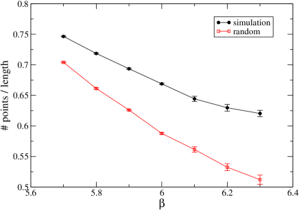
Figure 9: (line) density of monopoles on the shortest connected line joining all monopole sites: lattice simulation (full symbols) and after randomly re-distributing the monopoles (open symbols).

It is interesting that the $Z_{3}$ monopole density (of the Laplacian gauge) diverges in a somewhat controlled way: a situation where the $Z_{3}$ monopoles lie dense on 2d hypersurfaces of the 4d space-time would correspond to the observed scaling with the lattice spacing. In order to get a rough idea of how the the monopoles are organized within space, a closed loop which joins all monopole sites is calculated. This loop is obtained by a simulated annealing procedure which minimizes the length of the loop. Thereby, the Euclidean norm (where in addition the toroidal topology is taken into account) is used as a measure for lengths. From a mathematical point of view, finding the global minimum is a “traveling salesman” problem in three dimensions, and is beyond the reach of numerical calculation. However, the “simulated annealing” algorithm generically generates paths the length of which is within a few percents of the minimal length. This suffices for our purposes here. Given a finite set of points, it is difficult to tell whether the points are falling on top of a “smooth” curve. In order to gain first insight, we have calculated a connecting loop for a given set of $Z_{3}$ monopoles with the help of simulated annealing. Dividing the number of monopoles by the length of this loop gives an effective line density. Finally, this quantity is averaged over several lattice configurations. In order get a clue about the significance of this average line density, we have randomly re-distributed the monopoles of a particular configuration and we have re-calculated the effective line density. If the monopoles produced by the lattice simulation tend to fall on top of a smooth line, the average line density must be significantly larger than in the case of the random distribution of the same amount of monopoles. This is indeed the case, as is shown by figure 9.

6 Conclusions

MCG vortices of the gauge group $SU(2)$ have been realized as sensible degrees of freedom in the continuum limit [6], and they are closely related to confinement [3]. In the present paper, the MCG vortex matter has been investigated for the important case of $SU(3)$, using large-scale numerical simulations. Focal points were the questions: To which extent are the $SU(3)$ vortices relevant for confinement? Are the $SU(3)$ vortices meaningful in the continuum limit?

In a first step, we verified that the phase of large Wilson loops is represented by the center flux going through the Wilson loop. we confirmed the conjecture in [26] that the $Z_{3}$ fluxes going through a planar area are strongly correlated at length scales smaller than the hadronic one. As a byproduct, the flux correlation length (see (53) for a proper definition)

$$L_{1/2}\;\approx\;0.8\;\mathrm{fm}$$

was seen to be in rough agreement with scaling.

In a second step, the static quark potential produced by the MCG vortices was addressed. In contrast to the case of $SU(2)$, the string tension from the vortex projected ensembles turned out to be 62% of the full string tension. This finding is rather independent of the lattice size and the value of the lattice spacing. On the other hand, removing the $Z_{3}$ vortex degrees of freedom “by hand” from the full lattice configurations (see (39)), always results in a vanishing string tension (if the physical lattice volume is large enough). This implies that there is still a certain relation between the MCG vortices and confinement.

On the other hand, it is known [24, 25] that vortices which are defined from the Laplacian center gauge (LCG) reproduce the string tension to full extent. Here, we checked that “preconditioning” the lattice configurations with LCG and subsequent MCG fixing does not produce vortex matter which yields significantly more than 62% string tension.

The question arose as to which definition (MCG or LCG) of the vortices produces vortex structures which are sensible in the continuum limit. Here, the planar vortex density $\rho_{\mathrm{vor}}$ (the density of points where the vortices intersect a 2D planar hypersurface) as well as the (volume) density $\rho_{\mathrm{mon}}$ of $Z_{3}$ monopoles were studied. we found that in the case of the MCG vortices both quantities properly extrapolate to the continuum:

$$\frac{\rho_{\mathrm{vor}}}{\sigma}\;\approx\;0.45\;,\hbox to28.45274pt{\hfill}\frac{\rho_{\mathrm{mon}}}{\sigma^{3/2}}\;\approx\;0.35\;,\hbox to28.45274pt{\hfill}\frac{\rho_{\mathrm{mon}}}{\rho^{3/2}_{\mathrm{vor}}}\;\approx\;1.16\;.$$

In contrast, both quantities diverge in the continuum limit for the case of LCG vortices. Surprisingly, the LCG vortex matter satisfies simple scaling laws:

$$\rho_{\mathrm{mon}}\;a^{3}(\beta)\;\approx\;0.38\;a\;\sqrt{\sigma}\;,\hbox to28.45274pt{\hfill}\frac{\rho_{\mathrm{mon}}}{\rho^{3/2}_{\mathrm{vor}}}\;\approx\;0.9\hbox to56.9055pt{\hfill(LCG) }\;.$$

The investigations of sets of $Z_{3}$ monopoles residing within the spatial hypercube indicated that the LCG monopoles tend to fall on top of a “smooth” 1d curve which is embedded in this hypercube.

In summary, only the maximal center gauge allows for a direct interpretation of the vortices in the continuum limit of pure $SU(3)$ gauge theory. There is no string tension without MCG vortices, but MCG vortices only support 62% of the full value.

References

- [1] G. S. Bali, K. Schilling and C. Schlichter, Phys. Rev. D 51, 5165 (1995) [arXiv:hep-lat/9409005].
- [2] M. Lüscher and P. Weisz, JHEP 0207, 049 (2002) [arXiv:hep-lat/0207003].
- [3] J. Greensite, Prog. Part. Nucl. Phys. 51, 1 (2003) [arXiv:hep-lat/0301023].
- [4] L. Del Debbio, M. Faber, J. Greensite and S. Olejnik, Phys. Rev. D 55, 2298 (1997) [arXiv:hep-lat/9610005].
- [5] L. Del Debbio, M. Faber, J. Giedt, J. Greensite and S. Olejnik, Phys. Rev. D 58, 094501 (1998) [arXiv:hep-lat/9801027].
- [6] K. Langfeld, H. Reinhardt and O. Tennert, Phys. Lett. B 419, 317 (1998) [arXiv:hep-lat/9710068].
- [7] K. Langfeld, H. Reinhardt and A. Schafke, Phys. Lett. B 504, 338 (2001) [arXiv:hep-lat/0101010].
- [8] M. Creutz, Phys. Rev. D 21, 2308 (1980).
- [9] N. Cabibbo and E. Marinari, Phys. Lett. B 119, 387 (1982).
- [10] M. Albanese et al. [APE Collaboration], Phys. Lett. B 192, 163 (1987).
- [11] M. Teper, Phys. Lett. B 183, 345 (1987).
- [12] G. S. Bali and K. Schilling, Phys. Rev. D 46, 2636 (1992).
- [13] J. D. Stack, W. W. Tucker and R. J. Wensley, Nucl. Phys. B 639, 203 (2002).
- [14] J. Fingberg, U. M. Heller and F. Karsch, Nucl. Phys. B 392, 493 (1993) [arXiv:hep-lat/9208012].
- [15] G. S. Bali and K. Schilling, Phys. Rev. D 47, 661 (1993) [arXiv:hep-lat/9208028].
- [16] K. Langfeld, O. Tennert, M. Engelhardt and H. Reinhardt, Phys. Lett. B 452, 301 (1999) [arXiv:hep-lat/9805002].
- [17] M. Engelhardt, K. Langfeld, H. Reinhardt and O. Tennert, Phys. Rev. D 61, 054504 (2000) [arXiv:hep-lat/9904004].
- [18] M. Engelhardt and H. Reinhardt, Nucl. Phys. B 585, 591 (2000) [arXiv:hep-lat/9912003].
- [19] K. Langfeld, Phys. Rev. D 67, 111501 (2003) [arXiv:hep-lat/0304012].
- [20] M. Faber, J. Greensite and S. Olejnik, JHEP 9901, 008 (1999) [arXiv:hep-lat/9810008].
- [21] V. G. Bornyakov, D. A. Komarov and M. I. Polikarpov, Phys. Lett. B 497, 151 (2001) [arXiv:hep-lat/0009035].
- [22] R. Bertle, M. Faber, J. Greensite and S. Olejnik, Nucl. Phys. Proc. Suppl. 94, 482 (2001) [arXiv:hep-lat/0010058].
- [23] J. C. Vink and U. J. Wiese, Phys. Lett. B 289, 122 (1992) [arXiv:hep-lat/9206006].
- [24] C. Alexandrou, M. D’Elia and P. de Forcrand, Nucl. Phys. Proc. Suppl. 83, 437 (2000) [arXiv:hep-lat/9907028].
- [25] P. de Forcrand and M. Pepe, Nucl. Phys. B 598, 557 (2001) [arXiv:hep-lat/0008016].
- [26] J. Greensite and S. Olejnik, JHEP 0209, 039 (2002) [arXiv:hep-lat/0209088].
- [27] M. Faber, J. Greensite and S. Olejnik, Phys. Lett. B 474, 177 (2000) [arXiv:hep-lat/9911006].
- [28] A. Montero, Phys. Lett. B 467, 106 (1999) [arXiv:hep-lat/9906010].
- [29] M. Faber, J. Greensite and S. Olejnik, JHEP 0111, 053 (2001) [arXiv:hep-lat/0106017].
- [30] C. Alexandrou, P. de Forcrand and E. Follana, Phys. Rev. D 65, 114508 (2002) [arXiv:hep-lat/0112043].
- [31]