Hamiltonian Study of Improved $U(1)$ Lattice Gauge Theory in Three Dimensions

Abstract

A comprehensive analysis of the Symanzik improved anisotropic three-dimensional $U(1)$ lattice gauge theory in the Hamiltonian limit is made. Monte Carlo techniques are used to obtain numerical results for the static potential, ratio of the renormalized and bare anisotropies, the string tension, lowest glueball masses and the mass ratio. Evidence that rotational symmetry is established more accurately for the Symanzik improved anisotropic action is presented. The discretization errors in the static potential and the renormalization of the bare anisotropy are found to be only a few percent compared to errors of about 20-25% for the unimproved gauge action. Evidence of scaling in the string tension, antisymmetric mass gap and the mass ratio is observed in the weak coupling region and the behaviour is tested against analytic and numerical results obtained in various other Hamiltonian studies of the theory. We find that more accurate determination of the scaling coefficients of the string tension and the antisymmetric mass gap has been achieved, and the agreement with various other Hamiltonian studies of the theory is excellent. The improved action is found to give faster convergence to the continuum limit. Very clear evidence is obtained that in the continuum limit the glueball ratio $M_{S}/M_{A}$ approaches exactly 2, as expected in a theory of free, massive bosons.

I Introduction

Lattice gauge theory calculations have demonstrated important qualitative features of QCD, with increasing accuracy. Most lattice gauge theory calculations to date have been performed using Monte Carlo techniques in the Euclidean formulation. Although the Euclidean lattice gauge theory has been a very successful non-perturbative technique to compute the properties of elementary particles over the years, there are areas where progress has been very slow. Examples are QCD at finite temperature, glue thermodynamics, heavy quark spectra etc. Some of these problems have resisted solution even by the powerful techniques of Euclidean field theory. This suggests that alternative methods should be pursued in parallel with Euclidean lattice gauge theory. A viable alternative that needs to be explored is the Hamiltonian version of QCD. This approach provides a valuable check of the universality of the Euclidean results hamer96 and has an appealing aspect in reducing lattice gauge theory to a many-body problem. As such the formalism is suited for the application of a host of analytic methods imported from quantum many body theory and condensed matter physics. It has been suggested that Hamiltonian lattice gauge theory could more readily handle finite density QCD gregory00 . The problems encountered in finite density QCD in the Euclidean formulation have prompted a return to the strong coupling expansions of early Hamiltonian lattice gauge theory bringoltz02 . Similar ideas have been pursued recently by Luo et al., luo02 ; guo02 who propose an alternative Hamiltonian lattice formulation, ‘the Monte Carlo Hamiltonian’, and have already demonstrated its validity and efficiency for the $\Phi^{4}$ model huang02 .

Here we attempt to extend the standard Euclidean path integral Monte Carlo techniques to Symanzik improved $U(1)$ gauge theory in three dimensions. Applications of this method have been extremely successful cre79 ; cre83 and have given rise to great optimism about the possibility of obtaining results relevant to continuum physics from Monte Carlo simulations of lattice versions of the corresponding theory. Such an optimistic view is supported by recent work of Sexton et al. sexton95 , Boyd et al. boyd96 , Luo et al. xqluo00 and Morningstar and Peardon morn99a who have attempted to derive masses of the low-lying hadrons from such calculations and report successful results. More recent is the application of PIMC techniques to obtain results in the Hamiltonian limit for the $U(1)$ model in (2+1) dimensions mushe02 and SU(3) lattice gauge theory in (3+1) dimensions on anisotropic lattices tim03 .

The use of improved actions symanzik83 ; lusher85 makes possible accurate Monte Carlo simulations of QCD on coarse lattices with greatly reduced computational effort morn99a ; morningstar97 ; morningstar99b . In principal, with an improved action it is possible to achieve lattice volumes large enough to overcome finite-size effects and obtain measurements with good statistical errors. Coupled with tadpole improvement lepage93 , the pursuit of the Symanzik program has led to significant progress in reducing the discretization errors and the renormalization of the anisotropy to the level of a few percent; makes using anisotropic lattices no more this difficult than isotropic ones. At the same time the merits of using an improved anisotropic lattice have been well understood morningstar97 ; sakai00 . Anisotropic lattices allow us to carry out numerical simulations with a fine temporal resolution while keeping the spatial lattice spacing coarse, i.e., $a_{t}<a_{s}$, where $a_{t}$ and $a_{s}$ are the lattice spacings in the temporal and spatial directions, respectively. This is especially important for QCD Monte Carlo simulations at finite temperature and heavy particle spectroscopy. But more importantly it should make extrapolations to the continuum limit more reliable.

As mentioned above, our aim in this work is to apply standard Euclidean path integral Monte Carlo techniques to extract the Hamiltonian limit for Symanzik improved $U(1)_{2+1}$ lattice gauge theory on anisotropic lattices. The idea is to measure physical quantities on increasingly anisotropic lattices, and make an extrapolation to the extreme anisotropic limit. The effect of the plaquette improvement is examined by studying the scaling behaviour and the sensitivity of scaling coefficients of the string tension and glueball masses in the Hamiltonian limit, $\xi\rightarrow 0$. The rest of the paper is organized as follows: In Sec. II we briefly review the formulation of the Symanzik improved $U(1)$ gauge action in three dimensions on an anisotropic lattice. The details of the simulations and the methods used to extract the observables are described in Sec. III. Here we discuss our techniques for calculating the static quark potential, renormalization of anisotropy, string tension and glueball masses from Wilson loop operators. We present and discuss our results in Sec. IV. Scaling of the string tension, antisymmetric mass gap and the mass ratio in the weak-coupling region, are tested against theoretical predictions and compared with the estimates obtained by other studies in the Hamiltonian limit. Our conclusions are given in Sec. V, along with an outline of future work.

II Improved Anisotropic Discretization of $U(1)_{2+1}$

The Symanzik improved $U(1)_{2+1}$ gauge action on an anisotropic lattice is identical in form to the SU(3) case and is given by morningstar97

$$S_{g} = \beta_{s}\xi\sum_{x}\sum_{i<j}\left[\frac{5}{3u^{4}_{s}}P_{ij}(x)-\frac{1}{12u^{6}_{s}}\big{(}R_{ij}(x)+R_{ji}(x)\big{)}\right]$$ (1)

$$+\frac{\beta_{t}}{\xi}\sum_{x}\sum_{i}\left[\frac{4}{3u^{2}u^{2}_{t}}P_{it}(x)-\frac{1}{12u^{4}_{s}u^{2}_{t}}R_{it}(x)\right],$$

where $P_{\mu\nu}$ and $R_{\mu\nu}$ are the $1\times 1$ Wilson loop and $2\times 1$ rectangular loop in the $\mu\times\nu$ plane respectively. At the tree-level the coefficients are chosen so that the action has no $O(a^{2})$ discretization corrections. The spatial and temporal square and rectangular loops are given by

$$P_{ij}(x) = \left[1-U_{i}(x)U_{j}(x+\hat{i})U^{\dagger}_{i}(x+\hat{j})U^{\dagger}_{j}(x)\right]$$ (2)

$$R_{ij}(x) = \left[1-U_{i}(x)U_{i}(x+\hat{i})U_{j}(x+2\hat{i})U^{\dagger}_{i}(x+\hat{i}+\hat{j})\right.$$ (3)

$$\left.\times U^{\dagger}_{i}(x+\hat{j})U^{\dagger}_{j}(x)\right]$$

$$P_{it}(x) = \left[1-U_{i}(x)U_{t}(x+\hat{i})U^{\dagger}_{i}(x+\hat{t})U^{\dagger}_{t}(x)\right]$$ (4)

$$R_{it}(x) = \left[1-U_{i}(x)U_{i}(x+\hat{i})U_{t}(x+2\hat{i})U^{\dagger}_{i}(x+\hat{i}+\hat{t})\right.$$ (5)

$$\left.\times U^{\dagger}_{i}(x+\hat{t})U^{\dagger}_{t}(x)\right],$$

where $x$ labels the sites of the lattice, $i$, $j$ are the spatial indices and $U_{i}(x)$ is the link variable from site $x$ to $x+\hat{i}$. The rectangular loop that extends two steps in the time direction has not been included in the above action. This has the advantage of eliminating negative residue high energy poles in the gluon propagator morningstar97 but at the same time leaves errors of the order $a^{2}_{t}$ in the action. The $O(a^{2}_{t})$ errors, however, are negligible provided $a_{t}$ is small compared to $a$. The bare anisotropy parameter is $\xi$ and is equal to the aspect ratio of the temporal and spatial lattice spacings at the tree level. At higher orders in the perturbative expansion, the bare anisotropy in the simulated action is not the same as the measured value, $\xi_{phys}$, due to quantum corrections. The couplings $\beta_{s}$ and $\beta_{t}$ are defined by

$$\beta_{s}=\frac{1}{g^{2}_{s}},\hskip 28.45274pt\beta_{t}=\frac{1}{g^{2}_{t}}$$ (6)

The two different couplings in Eq. (1) are necessary in order to ensure that in the continuum limit, physical observables become independent of the kind of lattice regularization chosen. In the case of an asymmetric lattice, this implies that physical quantities have to be independent of the anisotropy factor $\xi$. To achieve this one needs to introduce different couplings for spatial and temporal directions, which depend on $\xi$. The $\xi$-dependence of the couplings $g^{2}_{s}$ and $g^{2}_{t}$ is due to quantum corrections and leads to an energy sum rule for the quark-antiquark potential, and the glueball mass, which differs in an important way from that which one would expect naively.

In the weak coupling limit of $SU(N)$ lattice gauge theory, the relation between the scales of the couplings in Euclidean and Hamiltonian formulations has been determined analytically from the effective actions Karsch82 ; hasenfratz81 ; kawai81 ; hamer95 , using the background field method on the lattice. For small values of $g_{E}$, the couplings $g_{s}$ and $g_{t}$ can be expanded as

$$\frac{1}{g^{2}_{t}} = \frac{1}{g^{2}_{E}}+c_{t}(\xi)+O(g^{2}_{E})$$ (7)

$$\frac{1}{g^{2}_{s}} = \frac{1}{g^{2}_{E}}+c_{s}(\xi)+O(g^{2}_{E})$$ (8)

where $g_{E}$ is the Euclidean coupling. For $\xi=1$, one recovers the usual Euclidean lattice gauge theory, where $g_{s}=g_{t}=g_{E}$. In the limit $\xi\rightarrow 0$, Eqs. (7) and (8) reduce to their Hamiltonian values and one obtains the relation between the Euclidean coupling $g_{E}$ and its Hamiltonian counterpart $g_{H}$. Similar calculations have been performed to determine the anisotropic coefficients $c_{s}$ and $c_{t}$ at arbitrary anisotropy for a class of improved actions margarita97 ; sakai99 ; engels00 ; sakai00 . These coefficients become an important tool in the analysis of glue thermodynamics hashimoto93 , the quark-gluon plasma nakamura96 ; nakamura98 and for the determination of spectral functions at finite temperature forcrand98 . Similar calculations have not yet been done for the $U(1)$ theory, however, as far as we are aware.

Tadpole improvement lepage93 is introduced by renormalizing the link variables: $U_{i}(x)\rightarrow U_{i}(x)/u_{s}$, and $U_{t}(x)\rightarrow U_{t}(x)/u_{t}$, where the mean fields $u_{s}$ and $u_{t}$ can be defined by using the measured values of the average plaquettes in a simulation. In the plaquette mean-link formulation, the mean fields are determined self-consistently and are defined by

$$u_{s}=(P_{ij})^{1/4},\hskip 14.22636ptu^{2}_{t}u^{2}_{s}=P_{it}.$$ (9)

For $a_{t}<<a$, the mean temporal link $u_{t}$ is expected to be very close to unity. For simplicity we use a convenient and gauge invariant definition for $u_{s}$ in terms of the mean spatial plaquette given by $u_{s}=\langle\mbox{Re}P_{ij}\rangle^{1/4}$, and compute $u_{t}$ from the temporal plaquette $P_{it}$ in Eq. (9).

To obtain the Hamiltonian estimates from anisotropic lattices, a naive extrapolation procedure is followed. In this procedure we assume classical values of the couplings, i.e., $\beta=\beta_{s}=\beta_{t}$ in Eq. (1) and extrapolate the physical quantities to the extreme anisotropic limit, $\xi\rightarrow 0$ at constant $\beta$. Such a procedure is not strictly correct, however, at the quantum level because $\beta_{s}\neq\beta_{t}\neq\beta$ due to renormalization.

As an example of the application of PIMC to the Symanzik improved action, we consider the case of compact $U(1)$ gauge theory in three dimensions. The relevance of the model to QCD at finite temperature ham94 has made it a standard proving ground for Hamiltonian lattice numerical methods. The model has two essential features in common with QCD, confinement pol77 ; pol78 ; gof82 ; ban77 and chiral symmetry breaking fiebig90 . Other common features are the existence of a mass gap and a confinement-deconfinement phase transition at some non-zero temperature. These similarities suggest that a comparison of the respective mass spectra should be informative. In the continuum limit of theory, the mass gap $M$ is found to behave as pol78

$$M^{2}a^{2}\approx\mbox{const.}\beta\mbox{exp}[-2\pi^{2}\beta v(0)]=M^{2}_{D}$$ (10)

where $v(0)\approx 0.2527$ is the lattice Coulomb Green’s function at zero separation. In Hamiltonian theory in which the space dimensions are discretized, $v_{H}(0)\approx 0.3214$ is the analogous Green’s function gof82 . It has been shown analytically that a linear confinement persists for all non-vanishing couplings, no matter how weak pol78 ; gof82 . The string tension as a function of coupling also scales exponentially and obeys a lower bound

$$K\geq\mbox{const.}M_{D}\beta^{-1}.$$ (11)

An interesting feature to explore in this context is whether the coupling to matter fields will change the permanent confinement status in (2+1) dimensions smorgrav03 .

III Method

III.1 Simulation details

To extract estimates of the string tension and the glueball masses using the Symanzik improved action in Eq. (1), a set of simulations are performed on lattices of size $N^{2}_{s}\times N_{t}$, ($N_{s}=16$, and $N_{t}=16-64$) where $N_{s}$ and $N_{t}$ are the number of lattice sites in the spatial and temporal directions respectively. The lattice size in the time direction is adjusted according to the anisotropy used in order to keep the physical length in the spatial and temporal directions equal. To analyse the behaviour in the strong and weak coupling regions, gauge configurations are generated using the Metropolis algorithm, for a range of couplings $\beta=1-2.5$. The details of the algorithm are discussed elsewhere mushe02 . Starting from an arbitrary initial gauge configuration, 50,000 sweeps are performed for the equilibration of the configurations and the self-consistent determination of the mean-field parameters. A Fourier acceleration procedure batrouni85 ; davis90 is used to overcome the stiffness against variations in the temporal plaquettes for high anisotropies. About 50$\%$ of the ordinary Metropolis updates are replaced with Fourier updates for $\xi\leq 0.4$ and about 100,000 further sweeps are performed to allow the system to equilibrate.

After thermalization, configurations are stored every 300 sweeps; 1200 stored gauge configurations are used in the measurement of the static quark potential and string tension and 1500 configurations for the glueball masses at each $\beta$. Measurements made on the stored configurations are binned into five blocks with each block containing an average of 250 measurements. The mean and standard deviation of the final observables are estimated simply by averaging over the block averages. The simulation parameters used for each configuration set are shown in Table 1.

Table 1: Simulation parameters at various $\beta$ and $\xi$ vales.

Volume	$\beta$	$\xi$	$u_{t}$	$u_{s}$	$(u_{s})^{4}$	$<P>\mbox{at}\hskip 1.13791ptu_{s}$
$16^{2}\times 32$	1.0	0.5	0.9991(3)	0.9218(2)	0.7220	0.7221(4)
$16^{2}\times 32$	1.45	0.5	0.9991(2)	0.9468(2)	0.8038	0.8039(3)
$16^{2}\times 32$	1.75	0.5	0.9997(3)	0.9551(3)	0.8324	0.8325(6)
$16^{2}\times 32$	2.0	0.5	1.	0.9589(2)	0.8458	0.8459(4)
$16^{2}\times 32$	2.5	0.5	1.	0.9614(4)	0.8543	0.8544(3)
$16^{2}\times 40$	1.0	0.4	1.	0.9182(3)	0.7110	0.7111(4)
$16^{2}\times 40$	1.45	0.4	1.	0.9432(3)	0.7917	0.7918(7)
$16^{2}\times 40$	1.75	0.4	1.	0.9497(3)	0.8138	0.8139(5)
$16^{2}\times 40$	2.0	0.4	1.	0.9524(5)	0.8228	0.8229(5)
$16^{2}\times 40$	2.5	0.4	1.	0.9561(2)	0.8358	0.8359(2)
$16^{2}\times 48$	1.0	0.333	1.	0.9152(3)	0.7016	0.7017(5)
$16^{2}\times 48$	1.45	0.333	1.	0.9356(3)	0.7663	0.7664(4)
$16^{2}\times 48$	1.75	0.333	1.	0.9401(2)	0.7815	0.7816(6)
$16^{2}\times 48$	2.0	0.333	1.	0.9408(4)	0.7836	0.7837(4)
$16^{2}\times 48$	2.5	0.333	1.	0.9454(4)	0.7991	0.7992(3)
$16^{2}\times 64$	1.0	0.25	1.	0.9112(6)	0.6895	0.6892(3)
$16^{2}\times 64$	1.45	0.25	1.	0.9287(3)	0.7440	0.7439(4)
$16^{2}\times 64$	1.75	0.25	1.	0.9357(5)	0.7665	0.7663(5)
$16^{2}\times 64$	2.0	0.25	1.	0.9381(4)	0.7745	0.7738(6)
$16^{2}\times 64$	2.5	0.25	1.	0.9401(4)	0.7812	0.7811(3)

III.2 The inter-quark potential and string tension

The static quark potential $V({\bf r})$ is extracted from the expectation values of the time-like Wilson loops $W({\bf r},t)$, which are expected to behave as

$$W({\bf r},t)\approx\sum_{i}Z_{i}({\bf r})\mbox{exp}[-tV_{i}({\bf r})],$$ (12)

where the summation runs over the excited state contribution to the expectation value, and $i=1$ corresponds to the lowest energy contribution. To obtain the optimal overlap of Wilson loop (and glueball) operators with the lowest state, it is necessary to suppress the contamination from excited states. This is done by using a simple APE smearing method morningstar97 ; albanese87 ; takahashi01 which is implemented by the iterative replacement of the original spatial link variables by a smeared link. Following the single-link smearing procedure, every space-like link variable $U_{i}(x)$ on the lattice is replaced by

$$U_{i}(x)\rightarrow P_{U(1)}\left[\alpha U_{i}(x)+\sum_{j\neq i}\sum_{\pm}U_{j}(x)U_{i}(x\pm\hat{j})U^{\dagger}(x\pm\hat{i})\right]$$ (13)

where $U_{-i}\equiv U^{\dagger}(x-\hat{i})$ and $i$ and $j$ are purely spatial indices. $P_{U(1)}$ denotes the projection onto $U(1)$ and $\alpha$ is the smearing parameter. Operators constructed out of smeared links dramatically reduced the mixing with high frequency modes, thus removing the excited-state contamination in the correlation functions. The smearing fraction is fixed to $\alpha=0.7$ and ten iterations of the smearing process are used. To reduce the variance, we use the technique of thermal averaging nogueira00 ; mushe02 , which amounts to replacing the time-like link variables $U_{t}$ by their local averages. This technique was applied to all temporal links except those adjacent to the spatial legs of loops, which are not independent. The technique has a dramatic effect in reducing the statistical noise.

The values of the effective potential are measured from the logarithmic ratio of successive Wilson loops

$$V_{t}({\bf r})=-\mbox{ln}\left[\frac{W({\bf r},t+1)}{W({\bf r},t)}\right]$$ (14)

which is expected to be independent of $t$ for $t>0$. A plot of the effective potential is shown in Fig. 1 for $\beta=1.70$ and $\xi=0.4$ for various separations $\bf r$. The dashed lines indicate the plateau values at various separations. As a result of heavy smearing, a good plateau behaviour is seen at small $t$ values for $r=1$ through 7. For $r\geq 6$, we see that the signal is dominated by noise for $t>6$. We fix the fitting range to be, in most cases, $t=2$ to 6.

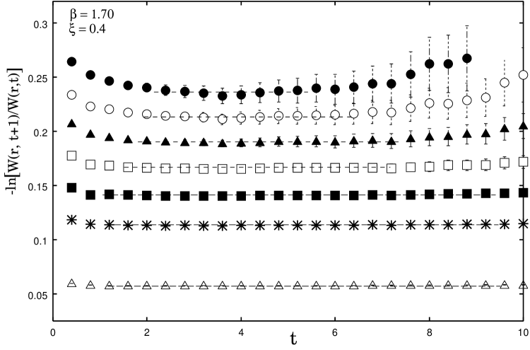
Figure 1: Effective potential as a function of Euclidean time $t$. From bottom up the horizantal lines correspond to $r=1$ through 7 and indicate the plateau values in the range $2\leq t\leq 6$.

The string tension is then extracted from the Wilson loops by establishing the linear behaviour for the static quark potential at large separation ${\bf r}$. We have chosen to fit our results for $V({\bf r})$ to the form gof82

$$V({\bf r})=a+K{\bf r}+b\mbox{ln}(\bf r),$$ (15)

where the linear term dominates the behaviour at large separations and a logarithmic Coulomb term dominates at small separations.

III.3 Renormalization of Anisotropy

Since the anisotropy ratio, $\eta$, is important in QCD simulations on the anisotropic lattices, we study its behaviour by numerical simulations. Measurements of renormalization of anisotropy norman98 have been made by comparing the static quark potential extracted from correlations along the different spatial and temporal directions. On an anisotropic lattice there are two different potentials $V_{t}(r)$ and $V_{s}(r)$ extracted from two different types of loops: time-like $W_{xt}$ and space-like $W_{xy}$ Wilson loops. The two potentials differ by a factor of $\xi_{phys}$ and by an additive constant, since the self-energy corrections to the static quark potential are different if the quark and anti-quark propagate along the temporal or a spatial direction. The natural way to proceed is to build ratios of the Wilson loops.

$$R_{t}(x,t) = \frac{W_{xt}(x,t+1)}{W_{xt}(x,t)}$$

$$R_{s}(x,y) = \frac{W_{xy}(x,y+1)}{W_{xy}(x,y)}$$ (16)

Asymptotically for large $\tau$ and $y$, the ratios $R_{t}$ and $R_{s}$ approach

$$R_{t}(x,t)\approx Z_{x\tau}\mbox{e}^{-\tau V_{t}}+(\mbox{excited state contr.})$$

$$R_{s}(x,y)\approx Z_{xy}\mbox{e}^{-yV_{s}}+(\mbox{excited state contr.})$$ (17)

The physical anisotropy is then determined from the ratio of the potentials $V_{t}(r)$ and $V_{s}(r)$ estimated from $R_{t}$ and $R_{s}$ respectively. The lattice potentials defined by Eq. (17) contain contributions from the self-energy terms. The potential is simply parameterized as

$$V_{s}(\xi,r)=V^{0}_{s}(\xi)+V^{f}_{s}(\xi,r),$$ (18)

where $V^{f}_{s}$ is the lattice potential free of self-energy contributions. The time-like potential $V_{t}$ is treated similarly. To eliminate the effect of the self-energy term $V^{0}$ in the potentials, we define a subtracted potential

$$V^{sub}_{s}(\xi,r,r_{0}) = V^{f}_{s}(\xi,r)-V^{f}_{s}(\xi,r_{0})$$

$$V^{sub}_{f}(\xi,t,t_{0}) = V^{f}_{t}(\xi,t)-V^{f}_{t}(\xi,t_{0})$$ (19)

where the subtraction points $r_{0}$ and $t_{0}$ are chosen to satisfy $t_{0}=\xi r_{0}$ and the matching of the potential $V^{f}_{t}(t_{0}=\xi r_{0})=V^{f}_{s}(r_{0})$ should be satisfied there. The subtraction radius $r_{0}$ should be chosen to be as small as possible so that fluctuations of the potential does not increase in which case simulations with high statistics on a larger lattice are required. The renormalized anisotropy is determined from the ratio

$$\xi_{phys}=\frac{V^{sub}_{t}(\xi,r,r_{0})}{V^{sub}_{s}(\xi,r,r_{0})}$$ (20)

and the measured anisotropy parameter, $\eta$, is then given by

$$\eta=\frac{\xi_{phys}}{\xi}$$ (21)

An alternative approach to make the comparison is to fit the measured potentials with the forms alford2001

$$a_{s}V_{s}(x) = a+\sigma a_{s}^{2}x+c\mbox{ln}x$$

$$a_{s}V_{t}(t) = a+\sigma a_{s}a_{t}t+c\mbox{ln}\left[\frac{a_{s}}{a_{t}t}\right]$$ (22)

The renormalized anisotropy $\xi_{phys}$ is then determined from the ratio of the coefficients of the linear terms in the two cases. It is advantageous to use the potential at smaller $r$, where the statistical errors are smaller, and determine $\xi_{phys}$ from the ratio of the coefficients of the Coulomb terms; however, such an estimate depends on short distance effects and is more sensitive to possible discretization errors of $O(a^{4}/r^{4})$ norman98 .

III.4 Glueball masses

The numerical analysis of the mass of a glueball having a given $J^{PC}$ proceeds through a study of the time-like correlations between space-like Wilson loop operators $\Phi_{i}(t)$

$$C(t)=\langle\bar{\Phi}^{\dagger}_{i}(t)\bar{\Phi}_{i}(t)\rangle,$$ (23)

where

$$\bar{\Phi}_{i}(t)=\Phi_{i}(t)-\langle 0\mid\Phi_{i}(t)\mid 0\rangle$$ (24)

is a gauge invariant vacuum subtracted operator capable of creating a glueball out of the vacuum. It is necessary to to subtract the vacuum contribution for the scalar glueball with $J^{PC}=0^{++}$, because in the large Euclidean time limit, $C(t)$ becomes dominated by the lowest energy state carrying the quantum numbers of $\Phi$ and these quantum numbers may coincide with that of the vacuum. The vacuum contribution is averaged over the whole ensemble before subtracting from the correlator. The glueball mass of interest is then extracted by studying the exponential decay of the correlation function for large Euclidean times, which is expected to behave as

$$C(t) = c_{i}\left[\mbox{exp}(-m_{i}t)+\mbox{exp}(-m_{i}(T-t))\right]$$ (25)

$$+(\mbox{excited state contributions})$$

where $m_{i}$ is the mass of the lowest-lying glueball which can be created by $\bar{\Phi}_{i}(t)$, and $T=N_{t}a_{t}$ is the extent of the periodic lattice in the time direction. Here, only the lowest “symmetric” ($PC=++$) and “antisymmetric” ($PC=--$) glueball states are studied. The measured values of $C(t)$ are expected to fall on a simple exponential curve assuming that the lattice is fine enough for the glueball mass to exhibit scaling behaviour according to the theoretical predictions.

On a finite lattice with lattice spacing $a$, the operator $\Phi_{i}(t)$ has a small overlap with the glueball ground state and the mass extracted from $C(t)$ may be too large owing to the excited-state contamination. The overlap gets worse as the lattice spacing is reduced and nears the continuum limit, $a\rightarrow 0$. This is obvious since the physical extension of the glueball remains fixed, while the operator $\Phi$, constructed from small loops, probes an ever smaller region of the glueball wave function as the lattice spacing is decreased. Hence it becomes important to use an improved glueball operator so as to have approximately the same size as the physical size of the glueball. For such an operator, the overlap with the glueball of interest is strong at small lattice spacing and signal-to-noise ratio is also optimal morningstar96 .

Following the variational technique of Morningstar and Peardon morningstar97 and the smearing procedure of Teper tep99 , an optimized operator was found as a linear combination of the basic operators $\phi$

$$\Phi(t)=\sum_{\alpha}v_{i\alpha}\phi_{i\alpha}(t)$$ (26)

where the index $\alpha$ runs over the rectangular Wilson loops with dimensions $l_{x}=[n-1,n+1]$, $l_{y}=[n-1,n+1]$ and smearing $n_{s}=[m-1,m+1]$. The correlation function $C(t)$ is then computed from the optimized glueball operator $\bar{\Phi}_{i}(t)$

$$C_{i}(t)=\sum_{t_{0}}\langle 0\mid\bar{\Phi}_{i}(t+t_{0})\bar{\Phi}_{i}(t_{0})\mid 0\rangle$$ (27)

Fig. 2 shows the effective mass plot for the scalar glueball for the measurements at $\beta=2.0$ and $\xi=0.50$. The signal is seen out to the time slice 6 and reaches a plateau region for $1\leq t\leq 5$. The data are noisy for $t>5$.

Figure 2: Effective mass plot for the scalar glueball at $\beta=2.0$ and $\xi=0.50$.

We choose to fit the correlation function $C(t)$ with the simple form

$$C_{i}(t)=c_{1}\cosh m_{i}[T/2-t]$$ (28)

to determine the glueball mass estimates.

IV Results and discussion

IV.1 Static quark potential and rotational symmetry

A plot of the static quark potential $V(r)$ as a function of $r$ at $\beta=1.55$ and $\xi=0.4$ is shown in Fig. 3. The data in this plot were obtained by looking for a plateau in the effective potential.

Figure 3: Static potential, $V(r)$, as a function of separation $r$ at $\beta=1.55$ and $\xi=0.4$. The solid line is a fit to the form $V(r)=a+br+c\mbox{ln}(r)$ in the range $3\leq r\leq 8$.

Because we are concerned to make long distance behaviour consistent in both fine and coarse directions, it is advantageous to use Wilson loops of the largest possible spatial extent. However, in practice, the statistical errors in large Wilson loops grow exponentially with separation. We use Wilson loops of size $8\times 8$ and fit the data by (15). We fit in the range $3\leq r\leq 8$ so that we are not sensitive to the Coulomb term and the discretization errors associated with it. We see that the data are fitted very well giving the string tension, $K(=\sigma a^{2})=0.044(3)$.

Figure 4: A close up of the static quark potential, $V(r)$, at small $r$, using the Symanzik improved action. The solid line is a fit of Eq. (15) to on-axis points $r=4$ to 8. This plot involves measurements at $\beta=1.55$ for $\xi=0.4$ with 10 smearing sweeps at smearing parameter $\alpha=0.7$

One of the main features of the improved discretization is the improved rotational invariance alford95 . Discretization errors in the gluon action affect the extent to which continuum symmetries, such as rotational symmetry, are restored. To explore the extent to which rotational invariance is improved, we measure the potential at off-axis as well as on-axis separations. Thus for improved rotational invariance, the static potential, for example, at ${\bf r}=(4,3)$ should agree exactly with that at ${\bf r}=(5,0)$.

For a fixed number of configurations and constant physical volume, we show the results from the Symanzik improved action and standard Wilson action in Figs. 4 and 5 respectively. We see that the off axis points for the improved lattice are excellently fitted by the rotationally invariant fitting curve (15) through $r=3$ to 8. The data from the Wilson action lie rather less close to the line of best fit. However, at large separations, the standard Wilson action does just as well as the improved action in extracting the static quark potential.

Figure 5: A close up of the static quark potential, $V(r)$, at small $r$. The solid line is a fit of Eq. (15) to on-axis points $r=4$ to 8. This plot involves measurements from the standard Wilson action mushe02 at $\beta=1.4142$ for $\xi=0.4$ with 10 smearing sweeps at smearing parameter $\alpha=0.7$.

As a quantitive measurement of the improvement, the potential measured in the simulation from non-planar Wilson loops is compared with an interpolation to the on-axis data norman98 :

$$\Delta V(r)\equiv\frac{V_{\mbox{sim}}(r)-V_{\mbox{fit}}(r)}{\sigma r}.$$ (29)

Results for ${\bf r}=(1,1)$ are given in Table 2. With the mean-field inspired Symanzik improvement, the difference is only a few percent compared to a difference of about 10-20% for the Wilson action mushe02 .

Table 2: Comparison between the measured anisotropy $\xi_{phys}$ and the input anisotropy $\xi$ for the Symanzik improved and the standard Wilson actions mushe02 . The measured difference in the off-axis potential at ${\bf r}=(1,1)$ are also shown.

Action	$\beta$	$\xi$	$\xi_{phys}$		$\Delta V(\sqrt{2})$
			$r_{0}=2$	$r_{0}=\sqrt{2}$
Improved	1.35	0.50	0.496(5)	0.493(2)	0.03(1)
action		0.40	0.392(4)	0.390(6)	0.03(2)
		0.333	0.328(3)	0.320(5)	0.04(4)
	1.45	0.444	0.442(6)	0.441(4)	0.04(2)
		0.333	0.326(3)	0.321(6)	0.04(3)
		0.25	0.246(4)	0.240(7)	0.05(4)
	1.55	0.40	0.402(2)	0.398(6)	0.04(2)
		0.25	0.241(5)	0.239(7)	0.06(4)
	1.65	0.333	0.334(5)	0.332(5)	0.02(1)
	1.75	0.25	0.252(4)	0.249(6)	0.03(1)
	2.0	0.333	0.335(6)	0.334(2)	0.03(1)
		0.25	0.242(4)	0.246(1)	0.06(2)
Wilson	1.35	0.444	0.418(5)	0.419(7)	0.12(1)
action	1.55	0.40	0.379(3)	0.374(6)	0.10(1)
	1.70	0.333	0.286(7)	0.289(5)	0.08(1)
	2.0	0.333	0.281(6)	0.292(2)	0.13(2)

IV.2 Numerical determination of renormalized anisotropy

We choose the points $r_{0}=2$ and $\sqrt{2}$ to compute the subtraction potentials of Eq. (19) and use them to obtain the ratio in Eq. (20). The subtracted spatial and temporal potentials at the subtraction point $r_{0}=\sqrt{2}$ are shown in Fig. 6. The anisotropies measured at these subtraction points for the improved and unimproved actions at different $\beta$ values are compared in Table 2. The two determinations of the anisotropies are in excellent agreement. These results show that the input anisotropy is normalized by less than a few percent for the improved action. This is in contrast with the standard Wilson action mushe02 , where the measured anisotropy is found to be about 20-30% lower than the input anisotropy $\xi$.

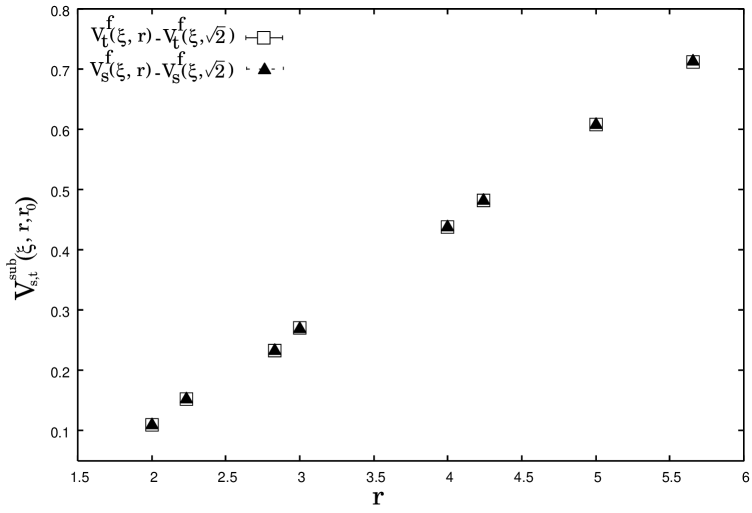
Figure 6: Subtracted spatial and temporal potentials against the separation $r$. This plot involves measurements at $\beta=1.75$ and $\xi=0.333$ for the subtraction point $r_{0}=\sqrt{2}$. The temporal potential $V^{sub}_{t}$ has been rescaled by the input anisotropy.

Fig. 7 shows the potentials computed from spatial and temporal Wilson loops without subtracting the self energy terms. We find that the difference between the estimates computed from subtracted and unsubtracted potentials is less than 1% for the Symanzik improved action. We conclude that a few percent renormalization in the anisotropy is sufficiently small that it is unlikely to represent the dominant effect in the final estimates and it is safe to use the bare anisotropy for the tadpole improved Symanzik action.

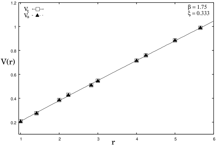
Figure 7: Unsubtracted spatial and temporal potentials against the separation $r$ at $\beta=1.75$ and $\xi=0.333$. The temporal potential $V_{t}(r)$ has been rescaled by the input anisotropy.

IV.3 String tension

To obtain estimates of the string tension in the Hamiltonian limit, an extrapolation is performed by a simple quadratic fit in powers of $\xi^{2}$ for each $\beta$ value. The simulations run over a range of anisotropies, $\xi=1-0.25$, thus enabling reliable extrapolation to the Hamiltonian limit. The errors for the extrapolation may be obtained by the “linear, quadratic, cubic” extrapolant method per00 . Fig. 8 shows our estimates of the string tension as a function of the anisotropy $\xi^{2}$ for various fixed $\beta$ values. Except at $\beta=1.35$, a fairly smooth variation of string tension with $\xi^{2}$ for various couplings is seen. The curvature in the extrapolation at $\beta=1.35$ suggests that our estimate may be somewhat too high there.

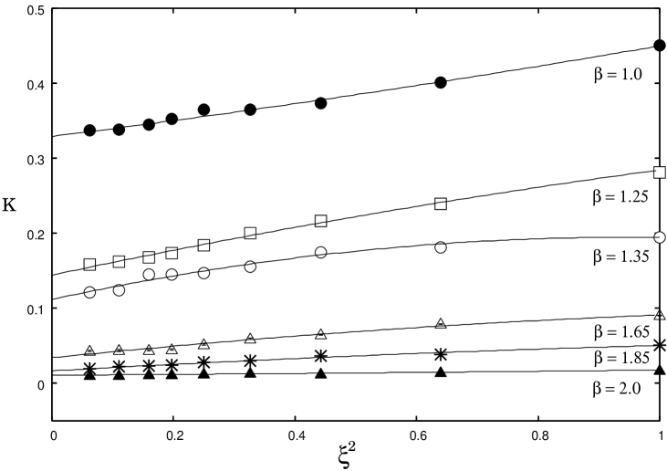
Figure 8: Extrapolation of the string tension to the Hamiltonian limit $\xi\rightarrow 0$, for various $\beta$. Solid lines show the quadratic fits in $\xi^{2}$ to the data.

Our extrapolated results for the string tension, $K=a^{2}\sigma$, together with the earlier Hamiltonian estimates obtained from the $t$-expansion mor92 , Green’s Function Monte Carlo simulations ham00 and the Exact Linked Cluster Expansion (ELCE) irv84 are plotted as a function of inverse coupling in Fig. 9. We see that the string tension displays an exponential behaviour at weak coupling in accordance with the theoretical prediction. It has rigorously been shown that the string tension in $U(1)_{(2+1)}$ undergoes a ‘roughening transition’ irv83 ; kogut81 at some intermediate coupling estimated to be near $\beta\approx 0.8$. Beyond the transition point, the different estimates of the string tension are expected to agree. The on-axis strong coupling series approximants fail to converge beyond $\beta=0.8$, which prevents the analytic continuation of the series expansion beyond the roughening transition. The $t$-expansion results, however, do not suffer from this difficulty. A comparison with the GFMC ham00 and an exact linked-cluster expansion irv84 and results shows that our estimates are in good agreement with earlier estimates. The $t$-expansion estimates mor92 are a little high, but still reasonably accurate. Of course, we do not expect that the results for the improved action should match exactly at finite coupling with other estimates which were computed for the unimproved action. We believe our PIMC estimates are more reliable and accurate and are also clearly consistent with the behaviour predicted by Polyakov pol78 and Göpfert and Mack gof82 .

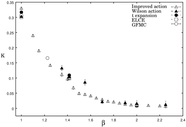
Figure 9: The string tension as a function of inverse coupling. Our present estimates are shown as open triangles. Earlier results from standard Wilson action mushe02 , $t$-expansion mor92 , Greens Function Monte Carlo simulations ham00 and an exact linked cluster expansion irv84 are shown as solid triangles, solid circles, open circles and open squares respectively.

Fig. 10 shows the scaling behaviour of the string tension together with results obtained using the standard Wilson action mushe02 , as a function of $\beta$. The dashed-dot line is the strong-coupling expansion to order $\beta^{4}$ hamer96a and the solid line represents a fit to the weak-coupling asymptotic form (6). It can be seen that our present estimates appear to match nicely onto the strong and weak coupling expansions in their respective limits. The $4th$ order strong coupling series expansion, obtained from integrated differential approximants, diverges beyond $\beta=1.30$. In the weak-coupling region, the string tension is consistent with the predicted scaling behaviour gof82 . An unconstrained fit of the form (6) represents the data rather well in the interval $1.45\leq\beta\leq 1.95$. The fit to the data gives a scaling slope of $3.04\pm 0.13$ and an intercept of $1.42\pm 0.21$. The intercept of the scaling curve is roughly two times larger in magnitude than the theory predicts, compared to our previous results with the standard Wilson action mushe02 which were higher than theory by a factor of 5 - 6. Also in contrast with the Wilson action, a significant reduction in the errors is clearly apparent with the tadpole-improved Symanzik action.

In summary, it appears that the overall exponential scaling behaviour is the same for both actions, but the constant coefficient is lower for the Symanzik action by a factor of 2 to 3, and closer to the theoretical weak-coupling estimate. It seems highly plausible that a different action should give a different renormalization for the constant coefficient, although no analytic calculation of this effect has been done.

Figure 10: The logarithm of the string tension as a function of inverse coupling. Our present estimates are shown as open triangles. The solid line is the result of fitting to form (6) for $1.45\leq\beta\leq 1.95$. The dash-dot line is the $\beta^{4}$ order strong coupling expansion hamer96a . Our previous estimates mushe02 are shown as solid triangles. The dashed line represents the finite size behaviour ham93 .

IV.4 Antisymmetric mass gap

The weak-coupling behaviour of the mass gap is not exactly known. The rigorous analysis of Göpfert and Mack gof82 showed that in the continuum limit $U(1)_{2+1}$ reduces to a massive scalar free field theory, with a mass gap $M$ which is expected to decrease exponentially as the lattice spacing goes to zero. They showed that the lattice photon mass in the Villain action on a 3-dimensional Euclidean lattice is given by Eq. (6). It is often claimed in the literature that the Villain action is a high-$\beta$ approximation of the Wilson action so that Eq. (6) should also hold in the weak-coupling limit of the Wilson model.

The extrapolation of the glueball masses to the Hamiltonian limit is shown in Fig. 11. The extrapolation is performed by using a simple quadratic fit in powers of $\xi^{2}$. Again we see a smooth dependence on $\xi^{2}$, for all $\beta$ values analysed here.

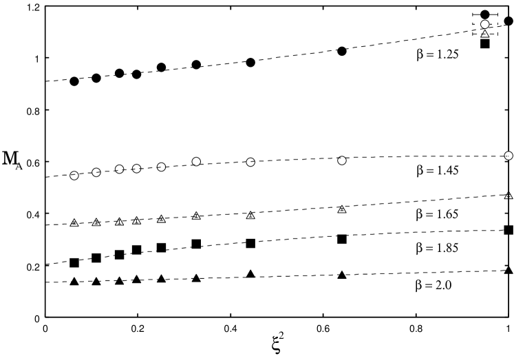
Figure 11: Extrapolation of the antisymmetric glueball mass to the Hamiltonian limit $\xi\rightarrow 0$. Dashed lines show the quadratic fits in $\xi^{2}$ to the data.

Our extrapolated results for the mass gap together with earlier Hamiltonian estimates obtained from the Wilson action mushe02 are plotted as a function of $\beta$ in Fig. 12. Unlike the string tension, the strong-coupling expansion of the mass gaps is believed to be analytic near the roughening point. Comparison with earlier Hamiltonian estimates shows that our present data follow quite closely the strong-coupling expansion estimates, obtained by the method of integrated differential approximants, in the strong and weak-coupling regions. The $t$-expansion estimates mor92 , obtained from D-Padé approximants, are found to be substantially less accurate than those from the SC-expansion. Beyond $\beta=2$, the approximants for the t-expansion do not converge well so that no reliable estimates can be obtained beyond that coupling value.

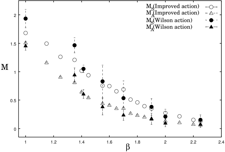
Figure 12: Glueball masses as functions of $\beta$. Our present results for the symmetric and antisymmetric glueball masses ($M_{S}$, $M_{A}$) are shown as open circles and triangles respectively. Earlier results obtained from the Wilson action mushe02 are shown as solid circles and triangles respectively.

Table 3: Comparison of the Hamiltonian results obtained for the symmetric and antisymmetric scalar glueball masses ($M_{S}$, $M_{A}$) for the Symanzik improved and Wilson actions.

$\beta$	Improved action		Wilson action
	$M_{S}$	$M_{A}$	$M_{S}$	$M_{A}$
1.0	1.68(1)	1.510(5)	1.9(1)	1.45(7)
1.35	1.207(9)	0.811(5)	1.4(1)	0.9(1)
1.55	0.75(1)	0.444(5)	0.8(2)	0.4(1)
1.70	0.69(2)	0.361(6)	0.5(3)	0.24(9)
1.90	0.352(6)	0.177(3)	0.3(1)	0.17(9)
2.0	0.272(4)	0.136(2)	0.2(1)	0.10(6)

The asymptotic scaling behaviour of the antisymmetric mass gap is shown in Fig. 13. The solid line is the result of fitting for $1.4\leq\beta\leq 2.25$ to the form (10) to find the scaling slope and the intercept of the scaling curve. Our results for these coefficients are shown and compared with previous studies in Table 4. These results are obtained by fitting to the form $M^{2}=\beta\mbox{exp}[-f_{0}\beta+f_{1}]$ in the weak-coupling region. It can be seen that the agreement with the earlier results is remarkable. We find the constant coefficient (intercept of the scaling curve) is approximately 1.5 times larger in magnitude than the theory predicts. This is an improvement over our previous estimate using the Wilson action mushe02 , where the constant coefficients were estimated a factor 5-6 times larger. The scaling slope is a little less than the theoretical prediction but in agreement with the estimates obtained in other numerical and analytic calculations (Ref. Table 4). Several studies have provided evidence that the antisymmetric mass gap in the Wilson model of $U(1)_{2+1}$ Hamiltonian lattice gauge theory does not fall in the weak-coupling limit in the same manner as the periodic Gaussian model. This may be a signal of non-universality for the Abelian $U(1)$ theory.

Figure 13: The logarithm of the antisymmetric mass gap as a function of $\beta$. Open triangles show our present estimates. The solid line is the fit to the data for $1\leq\beta\leq 2$. Previous estimates from the Wilson action mushe02 are shown as solid triangles.

Table 4: Results for the coefficients $f_{0}$ (slope of the scaling curve) and $f_{1}$ (the intercept of the scaling curve) in the weak-coupling limit for the antisymmetric mass gap.

Source	$f_{0}$	$f_{1}$
Villain (Hamiltonian) gof82	6.345	4.369
Morningstar mor92	5.23	5.94
Hamer and Irving hamer85a	5.30	6.15
Hamer, Oitmaa and Weihong ham92	5.42	6.27
Plaquette Expansion john97	5.01	5.82
Heys and Stump hey85	4.97	6.21
Lana lana88	4.10	4.98
Xiyan, Jinming and Shuohong fan96	5.0	5.90
Dabringhaus, Ristig and Clark dab91	4.80	6.26
Darooneh and Modarres dar2000	4.40	5.78
Present Work	5.39(9)	6.3(1)

IV.5 Mass gap ratio

The quantity of interest here is the dimensionless ratio $R_{M}$ between the symmetric and antisymmetric mass gap in the large $\beta$ limit. In this limit the ratio $R_{M}=M_{S}/M_{A}$ is expected to tend smoothly to its continuum value. In practice, this limiting value is found by increasing $\beta$ from strong-coupling until the mass ratio levels off in the weak coupling region. Earlier studies of the photon mass mor92 showed that the scaling of the mass ratio sets in for $\beta>1$. If the continuum theory admits a stable bound state of two photons (a glueball), then the weak-coupling limit of the mass ratio will lie between 1 and 2. If the continuum theory is simply a free-field theory of massive scalar photons, as in the Villain model or if the glueball remains in the continuum theory only as a resonance, then the ratio $R_{M}=2$ should be observed as $\beta$ becomes large. Lana lana88 argued for a sharp “transition point” at $\beta=1.40$ where the symmetric bound state ceases to be stable, and crosses the level consisting of two free axial particles, so that mass ratio suddenly levels out at value 2.

In general, the most accurately calculated physical quantity is the string tension $K$. Therefore the first quantity that we shall extrapolate to the continuum limit will be of the form $M/K$, where $M$ is the glueball mass. The leading corrections to such a ratio are known to be of the order $O(1/\zeta)^{2}$ tep99 , where $\zeta$ is some length scale. In the weak-coupling limit,

$$M_{A}/K\rightarrow\pi^{2}/2\hskip 11.38092pt\mbox{as}\hskip 8.5359pt\beta\rightarrow\infty,$$

in constrast to QCD, where $M/\sqrt{K}$ is constant in the continuum limit. Fig. 14 displays the estimates for this quantity, as a function of $\beta$. The data certainly appear to level out below $a^{2}_{eff}\approx 0.006$ at a value 6. This is quite close to the predicted value for the Villain model.

Figure 14: The dimensionless ratio $M_{A}/\beta K$ as a function of effective lattice spacing, $a_{eff}$. Open triangles show our present PIMC estimates. Our previous estimates using the Wilson action mushe02 are shown as solid triangles.

Figure 15 shows the behaviour of the dimensionless mass ratio $R_{M}=M_{S}/M_{A}$ as a function of effective lattice spacing squared, $a^{2}_{eff}$, where $a_{eff}$ is defined from Eq. (10) as mushe02

$$a_{eff}=\sqrt{8\pi^{2}\beta}e^{-\pi^{2}\beta v(0)}.$$

The plot shows that the mass ratio approaches very closely to the expected value of 2 in the large $\beta$ limit. A linear fit to the data from $0.00026\leq a^{2}_{eff}\leq 0.0066$ gives $R_{M}=2.007\pm 0.01$, which is consistent with a continuum limit value $R_{M}=2$. There is no sign of a stable, scalar glueball bound state, nor of any sharp ”break” in the mass ratio. In comparison with previous results using the unimproved action, there are two notable features. First, the results are much more accurate. Secondly, the corrections to the continuum limit appear to be linear in $a^{2}_{eff}$, whereas those for the unimproved action were linear in $a_{eff}$ mushe02 . This provides impressive evidence that the improved action has achieved what it was designed to do: produce faster convergence to the continuum limit.

Table 5: Comparison of the Hamiltonian estimates for dimensionless mass ratio $R_{M}$ obtained using the improved and standard Wislon actions

$\beta$	$R_{M}$
	Improved action	Wilson action
1.0	1.11(2)	1.32(1)
1.35	1.4(1)	1.5(2)
1.55	1.7(1)	2.1(1.1)
1.70	1.9(2)	2.2(1.5)
1.90	2.0(3)	2.2(1.5)
2.0	2.0(5)	2.4(1.6)

Figure 15: Mass ratio, $R_{M}$, as a function of effective lattice spacing, $a_{eff}$. Our present estimates are shown as the open triangles. The solid line is the fit to the data in the range $0.00026\leq a^{2}_{eff}\leq 0.0066$. The solid triangles show our earlier estimates obtained from the Wilson action mushe02 .

Table 6: PIMC results for the string tension, $K$, symmetric and antisymmetric glueball masses $M_{S}$, $M_{A}$ and the mass ratio $R_{M}$.

$\beta$	$a_{eff}$	$K$	$M_{S}/K$	$M_{A}/K$	$R_{M}$
1.0	0.3724	0.329(2)	5.10(5)	4.58(4)	1.11(2)
1.15	0.2481	0.189(3)	7.8(1)	6.1(1)	1.28(3)
1.25	0.1884	0.141(2)	8.9(2)	6.4(1)	1.38(4)
1.35	0.1425	0.112(5)	10.8(5)	7.3(4)	1.4(1)
1.40	0.1239	0.096(5)	10.4(5)	6.7(3)	1.6(1)
1.45	0.1076	0.067(4)	13.9(9)	8.0(5)	1.7(2)
1.55	0.0810	0.045(3)	16.6(1.0)	9.8(6)	1.7(1)
1.60	0.0702	0.041(2)	18.1(1.1)	10.1(6)	1.8(1)
1.65	0.0608	0.034(2)	19.3(1.3)	10.4(9)	1.8(2)
1.70	0.0527	0.028(2)	24.1(2.1)	12.6(1.0)	1.9(2)
1.75	0.0425	0.023(2)	22.0(2.2)	11.6(1.1)	1.9(3)
1.80	0.0395	0.021(2)	21.6(2.7)	11.1(1.3)	1.9(3)
1.85	0.0341	0.016(2)	23.4(2.5)	12.3(1.3)	1.9(3)
1.90	0.0295	0.013(2)	25.9(3.2)	13.0(1.6)	1.6(3)
2.0	0.0220	0.010(2)	26.0(4.5)	12.9(2.2)	2.0(5)
2.10	0.0164	0.009(2)	23.4(5.0)	11.5(2.5)	2.0(6)
2.20	0.0122	0.008(2)	18.9(8.7)	9.6(2.4)

V Summary and conclusions

In this work, we have applied the standard Euclidean path integral Monte Carlo method to obtain results in the Hamiltonian limit of the Symanzik improved $U(1)_{2+1}$ lattice gauge theory on anisotropic lattices. Monte Carlo results were obtained for the static quark potential, renormalized anisotropy, the string tension, and the lowest-lying glueball masses. The inter-quark potential with the improved action exhibits good rotational symmetry. We found that both the improved and standard Wilson action do equally well in extracting the static potential at large separations. The improved discretization allows substantially more accurate estimates of the string tension and the glueball masses. The extrapolations to the Hamiltonian limit were performed by simple quadratic fits.

In this limit the string tension displays an asymptotic behaviour which is in excellent agreement with the behaviour predicted by the weak-coupling approximation of Göpfert and Mack gof82 . The scaling coefficient of the scaling curve for the mass gap was estimated as roughly twice larger in magnitude than the weak-coupling prediction. This is an improvement over our previous unimproved results which were estimated larger by a factor of 5-6. We believe that these estimates can be further improved by taking the renormalization of the couplings into account, i.e, computing the action beyond the tree-level.

The weak-coupling behaviour of the antisymmetric mass gap was found to agree with the theoretical expectations. The parameters agree quite well with the results obtained from previous numerical and analytic calculations. The mass ratio $R_{M}=M_{S}/M_{A}$ was observed to scale to $2.007\pm 0.01$ in the continuum limit. No sign of a glueball bound state or a sharp crossover between the levels was seen. This is in excellent agreement with the statement of Göpfert and Mack gof82 , that the continuum limit corresponds to a theory of free bosons, where $R_{M}=2$ exactly. It also shows very clearly the value of using an improved action, in giving more rapid convergence to the continuum limit, as well as improved accuracy.

Taking advantage of the improved discretization on anisotropic lattices, we aimed to apply the Euclidean path integral Monte Carlo approach to examine the Hamiltonian limit of $U(1)$ theory. The results obtained here clearly demonstrate that PIMC is a more reliable technique than other quantum Monte Carlo methods, such as Green’s Function Monte Carlo, which gave only qualitative estimates of the string tension and the mass gap.

Although suffering from the disadvantage that it requires an extrapolation to the anisotropic limit, PIMC is the preferred Monte Carlo technique for obtaining reliable results in the Hamiltonian formulation, just as in the Euclidean formulation. In order to make the PIMC method a more valuable tool in Hamiltonian lattice gauge theories, it will be crucial to show that it allows one to treat eventually matter fields as well as gauge fields especially in the non-Abelian case.