Chaotic Quantization of Four-Dimensional U(1) Lattice Gauge Theory

Abstract

We demonstrate that the quantized U(1) lattice gauge theory in four Euclidean dimensions can be obtained as the long time average of the corresponding classical U(1) gauge theory in 4+1 dimensions. The Planck constant $\hbar$ is related to the excitation energy and the lattice constant of this classical template.

I Introduction

The nonlinear classical dynamics of gauge fields is known to be strongly chaotic MST81 ; BMM95 . The classical SU(2) gauge theory defined on a three-dimensional lattice has been studied numerically in considerable detail and was shown to be a globally hyperbolic (Anosov) system chaos . For such systems, any generic initial gauge field configuration wanders ergodically in the phase space of field configurations. This motion leads in the infrared limit to a stationary distribution of lower dimensional configurations BMM01 . These, as a result of the higher dimensional classical dynamics, are distributed exactly as required by the vacuum state of the Euclidean quantum theory on the lower dimensional space.

This phenomenon, which has been called chaotic quantization Beck95 ; BMM01 , can be simply considered as a physical realization of the method of stochastic quantization PW81 . It is a consequence of two deep relationships: (1) that the long time properties of certain deterministic classical systems can be described by the methods of statistical physics Dorfman , and (2) the correspondence between classical statistics and Euclidean quantum mechanics. In the appendix we demonstrate this correspondence for the quantum harmonic oscillator in detail.

According to the chaotic quantization scenario it is necessary for the higher dimensional (second time) dynamics to be chaotic in order to appear as a quantum theory in the lower (one-time) dimensions. From the investigation of the U(1) gauge theory presented in this article we shall see that the existence of the lattice is essential for this scenario to work in those cases when the dynamics would not be chaotic in the weak coupling limit. The chaotic quantization may fail for systems not being chaotic on finite lattices as well as in case of observing too short second-time of the dynamical evolution. This opens up towards the possibility that not all interactions, in particular gravity, have to be quantized in nature.

This way the chaotic quantization of gauge theories also lends support to ’t Hooft’s proposal tHooft that quantum mechanics could arise from an underlying dissipative, yet microscopically deterministic classical dynamics. We will not explore this speculative avenue here and confine ourselves to reporting our numerical evidence for a correspondence between the classical U(1) gauge theory in 4+1 dimensions and the quantum U(1) gauge theory in 4 dimensions.

The classical compact U(1) gauge theory without matter fields is the simplest gauge theory still exhibiting chaotic dynamics in calculations on three-dimensional lattices U1 . Although its continuum limit is not chaotic, in contrast to non-Abelian gauge theories where chaos survives even in this limit, the classical dynamics of the compact U(1) lattice gauge field is chaotic at finite lattice spacing $a$ and sufficiently strong coupling $g$ ($ga^{2}$ finite)BMM95 . As in the case of non-abelian gauge theories few mode models, like the $xy$-model XY-MODEL can be studied, a 3-link section of U(1) lattice gauge theory reveals a system of harmonically coupled pendulums, easy to see numerically drifting in chaotic behavior at high energy. The dimensionless parameter controlling the strength of chaoticity of the lattice gauge theory is $g^{2}aE_{p}$, where $E_{p}$ is the average total energy per elementary lattice plaquette.

Our conjecture of the correspondence between the (4+1)-dimensional classical gauge theory with chaotic dynamics and the 4-dimensional Euclidean quantum field theory can be expressed in the following relation between the 4-dimensional Planck constant $\hbar$ and two physical parameters of the higher dimensional classical theory: the temperature $T$ and the lattice spacing BMM01 :

$$\hbar=aT.$$ (1)

Our philosophy here views $\hbar$ as a constant of nature factorized into two underlying properties of the true (4+1)-dimensional world. An analogous case is the relation of classical electrodynamics factorizing the speed of light $c$ into electric and magnetic properties of the vacuum:

$$1/c^{2}=\epsilon_{0}\mu_{0}.$$ (2)

Taking the invariance of $c$ as an axiom in the theory of special relativity, one can derive the Lorentz transformation law without the need for any reference to electric or magnetic fields. Maxwell theory on the other hand, as a classical field theory, regards the dielectric constant $\epsilon_{0}$ and the magnetic permeability $\mu_{0}$ as independent properties of the physical vacuum. Light waves are solutions of the Maxwell theory, and the speed of light is calculable. The proposed relationship between quantum field theory and an underlying classical field theory in a higher dimension is analogous.

In this letter we report the results of numerical simulations of a U(1) lattice gauge theory both in 4 and 4+1 dimensions. The 4-dimensional Euclidean quantum gauge theory was simulated by standard quantum Monte-Carlo techniques. The 4+1-dimensional classical theory was simulated by numerical solution of the differential equations describing its Hamiltonian dynamics. In both cases, $4^{4}$ hypercubic lattices were employed. Lattice links beginning at point $x$ and pointing in the $\mu$ direction are associated with phases, $A_{\mu}(x)$, of unimodular complex numbers $U_{x,\mu}=\exp[igaA_{\mu}(x)]\in{\rm U}(1)$ in these theories.

II Classical and Quantum Lattice Gauge Models

In order to discuss the lattice regularization of classical and quantum field theory in parallel, we use a common notation as far as possible. Our starting point is the definition of the link variables $U$, which are always elements of the local U(1) group, but the interpretation, and hence the decomposition, of the phase can be different. In order to relate a physical interpretation to the lattice model phase, $gaA$, we consider the product of charge and vector potential, $qA$ (in the CGS system with $c=1$), which is the interaction energy associated with the field living on a link of length $a$ with a physical test charge $q$. This expression must be divided by another quantity with the dimension of an energy to generate a dimensionless phase variable. This quantity, the unit link energy $\epsilon$, is used as an energy “standard”, but it does not appear in the equations of motion of the theory. Also, we are free to choose $\epsilon$ differently in the quantum and in the classical theory. The general link variable is now given by

$$U_{L}=\exp(iqA/\epsilon).$$ (3)

In the standard quantum lattice gauge field theory the energy scale associated with a link of length $a$ is

$$\epsilon_{\rm Q}=\hbar/a.$$ (4)

In a classical theory, however, no reference to the Planck constant $\hbar$ is allowed. In this case we will use instead the Coulomb energy associated with two charges $q_{\rm K}$ at the endpoints of the link of length $a$, which in three spatial dimensions is given by

$$\epsilon_{\rm K}=q_{\rm K}^{2}/a.$$ (5)

By comparing the classical ($K$) and quantum ($Q$) systems of U(1) lattice gauge fields, we shall consider configurations characterized by the same link phase $gaA$. Using a common lattice spacing $a$ and a common coupling strength $g$, this convention naturally leads to the consideration of the same vector potential field, $A$, in the continuum limit. We can express this correspondence by the relation

$$q_{\rm Q}/\epsilon_{\rm Q}=q_{\rm K}/\epsilon_{\rm K}=ga.$$ (6)

As a consequence the classical charges as reference sources for the unit link energy are interpreted differently in the two cases: $q_{\rm Q}=g\hbar$ in the quantum theory and $q_{\rm K}=1/g$ in the classical lattice theory. In a sense, the two approaches are dual to each other, with $q_{\rm Q}q_{\rm K}=\hbar$, i.e. a high value of the charge corresponds to strong coupling in the quantum, but to weak coupling in the classical theory.

We note that the conventions chosen by us here are not unique. Alternative conventions, e.g. relating $\epsilon_{\rm K}$ to a classical charge in four spatial dimensions, as $\epsilon_{\rm K}=q_{d}^{2}/a^{2}$ are also possible, but they would not lead to different conclusions. In the end, the classical theory as well as the quantum theory are defined through the interactions of the dimensionless link variables $U$. The classical Hamiltonian $H_{\rm K}[U]$, being scale invariant, is a nonlinear function of the link variables, multiplied by a constant parameter carrying the dimension of energy. Likewise, the action of the quantum theory $S_{\rm Q}[U]$, which depends on the scale only through the gauge coupling $1/g^{2}(a)$ as an overall factor, has the dimension of an action. If, as we will show below, the two theories are related to each other, this implies a relationship between the dimensionful factors of $H_{\rm K}$ and $S_{\rm Q}$, which does not depend on the conventions used in the definition of the phase of $U$.

Physical quantities are related to the oriented product of link variables around an elementary square, a plaquette. Using the notion of lattice forward derivatives, $a\partial_{\mu}f=f(x+ae_{\mu})-f(x)$, (where $e_{\mu}$ is a unit vector in the corresponding direction) the plaquette phase sums are associated with the local rotations of the vector potential, with the field strength tensor

$$F_{\mu\nu}(x)=\partial_{\mu}A_{\nu}(x)-\partial_{\nu}A_{\mu}(x).$$ (7)

An elementary plaquette variable is related to a component of the field strength tensor:

$$U_{x,\mu\nu}=\exp\left(iga^{2}F_{\mu\nu}(x)\right),$$ (8)

and the lattice sum over all plaquettes

$$\Sigma_{\rm P}=\sum_{x}\sum_{\mu>\nu}\left(1-{\rm Re}\>{\rm tr}(U_{x,\mu\nu})\right)$$ (9)

is related to the physical energy or action, depending on the dimensionality of the considered space. For the U(1) group,

$$1-{\rm Re}\>{\rm tr}(U_{x,\mu\nu})=1-\cos\left(ga^{2}F_{\mu\nu}(x)\right),$$ (10)

which in the continuum limit $a\rightarrow 0$ approaches $(1/2)g^{2}a^{4}(F_{\mu\nu})^{2}.$ The plaquette sum approximates

$$\Sigma_{\rm P}\approx g^{2}a^{4}\sum_{x,\mu\nu}\frac{1}{4}F_{\mu\nu}^{2}(x).$$ (11)

Over a 4-dimensional lattice it is proportional to the action, $\Sigma_{\rm P}=g^{2}S_{4}$, and can be used to express the logarithmic weight of a configuration:

$$S_{4}/\hbar=\frac{1}{g^{2}\hbar}\>\Sigma_{\rm P}\;=\;\beta\Sigma_{\rm P},$$ (12)

where $\beta$ is a dimensionless constant playing the role of a (fictitious) temperature. Note that the fine structure constant can be expressed as $\alpha=q^{2}/4\pi\hbar$, yielding the familiar relation

$$\alpha_{\rm Q}=\frac{g^{2}\hbar^{2}}{4\pi\hbar}=\hbar\frac{g^{2}}{4\pi}=\frac{1}{4\pi\beta}$$ (13)

for quantum lattice gauge theory, and

$$\alpha_{\rm K}=\frac{1}{4\pi\hbar g^{2}}=\frac{\beta}{4\pi},$$ (14)

for the classical theory. The duality of these interpretations is manifest here, as well.

In the (4+1)-dimensional classical lattice gauge theory the summation over all plaquettes of a 4-dimensional spatial lattice is proportional to the (four-dimensional) magnetic energy. Since the classical interpretation cannot refer to the Planck constant, we arrive at the following expression for the energy by using $\epsilon_{\rm K}$ as the energy unit:

$$E_{5}^{\rm magn}=\epsilon_{\rm K}\Sigma_{\rm P}=\frac{1}{g^{2}a}\Sigma_{\rm P}.$$ (15)

Here we used (6) to eliminate $q_{\rm K}$ from the definition (5) of $\epsilon_{\rm K}$. In the continuum limit, the magnetic energy becomes

$$E_{5}^{\rm magn}\approx a^{4}\sum_{x,\mu\nu}\frac{1}{4a}F^{2},$$ (16)

confirming that the physical gauge fields in 4+1 dimensions, $A^{(4+1)}$ are related to those in 4 Euclidean dimensions, $A^{(4)}$, by a factor $a^{-1/2}$.

We now come to our main point. The conjecture $\hbar=aT$ is supported if the quantum and classical lattice simulations can be brought into a correspondence relating configuration weights, and thereby all physical expectation values, by

$$\exp(-S_{4}/\hbar)\propto\exp(-E_{5}^{{\rm magn}}/T)\propto\exp(-\beta\Sigma_{\rm P}).$$ (17)

We have used proportionality signs in this relation, because the overall normalization of the weights is not relevant. Also, the relation (17) defines the temperature $T$ as the equipartitioning energy for the magnetic energy of the classical lattice field. This designation obviously requires that the classical theory is ergodic, so that a single field trajectory generates configurations with a microcanonical equilibrium distribution.

Quantum Monte Carlo algorithms generate configurations of lattice link elements according to the Gibbs weight $w[U]\propto e^{-\beta\Sigma_{\rm P}}=e^{-S[U]/\hbar}$. The classical Hamiltonian approach, on the other hand, divides the Hamiltonian into its electric and magnetic parts:

$$H=a^{4}\sum_{x,\mu}\frac{1}{2a}\dot{A}^{2}+E^{\rm magn}[U].$$ (18)

This formula leads to the following dimensionless Hamiltonian lattice model, where the time is measured in lattice spacing units $a$ and time derivatives take the dimensionless form $a(\partial/\partial t)$:

$$g^{2}aH=\frac{1}{2}\sum_{\rm L}{\rm tr}\left(a\dot{U}a\dot{U}^{{\dagger}}\right)+\Sigma_{\rm P}.$$ (19)

Now the link variables $U_{x,\mu}$ are still defined on a four-dimensional lattice, but they are functions of an additional, continuous and scaled time variable $t/a$. The evolution of the lattice configuration occurs in this fifth dimension, usually called “fictitious” time in the context of stochastic quantization. In the present context, however, the time-like dimension is considered as physical, albeit unobservable at long distances and low frequencies. One reflection of this difference is that we do not add an external heat bath or white noise to the classical dynamical equations; we here consider pure classical Hamiltonian dynamics.

III Technical Aspects of the Simulations

We now explain some technical aspects of our simulations, before we report the results. For the purpose of generating generic initial field configurations, and as a matter of convenience, we prepared the initial configuration for the classical Hamiltonian simulation by Monte-Carlo “heating” on a five-dimensional lattice. The $\beta_{5}$ parameter chosen for this simulation determines the average value of the action $S_{5}$ and of the five-dimensional electric and magnetic energies. The selected configuration was then converted into the initial data for a four-dimensional, real-time lattice calculation as follows: The space-space-like plaquettes and links were taken without change from the four-dimensional hypercube located at $x_{5}=0$. The periodic boundary condition in the $x_{5}$-direction allowed us to identify the link phase for $x_{5}/a_{5}=-1$ with those at $x_{5}/a_{5}=N_{5}-1$ for the construction of the initial values for the time derivatives $\dot{U}$ on the hypercube in terms of the link variables attached to the plane $x_{5}=0$. This construction also used the link phases in the $x_{5}$ direction to make the time derivatives gauge covariant. By construction, the $\dot{U}$ variables then are orthogonal to the corresponding $U$ variables, as required by the Hamiltonian time evolution. We now present the details of our algorithm for the construction of the initial gauge field configurations.

We denote by $U_{+}$ the triple product of link variables including the value at $x_{5}/a_{5}=1$ (the first argument refers to the site coordinates $x=\{x_{1},\cdots,x_{4}\}$; the second argument indicates the value of $x_{5}/a_{5}$):

$$U_{+}=U_{5}(x,0)U_{x}(x,1)U^{{\dagger}}_{5}(x+a_{s},0)$$ (20)

and similarly by $U_{-}$ that product including the previous-time value

$$U_{-}=U^{{\dagger}}_{5}(x,-1)U_{x}(x,-1)U_{5}(x+a_{s},-1)$$ (21)

Both triples close a plaquette with the $U=U_{x}(x,0)$ link. These plaquettes encode the electric field values at $x_{5}\pm a_{5}/2$. Using the scalar product notation for U(1) group elements:

$$\langle A,B\rangle=\cos(\phi_{A}-\phi_{B}),$$ (22)

we can determine the electric field energy densities $\varepsilon_{\pm}=\frac{1}{2}E_{x}^{2}(x,\pm\frac{a_{5}}{2})$ as follows:

$$\langle U_{+},U\rangle = 1-(a_{5}a_{s})^{2}\varepsilon_{+},$$

$$\langle U_{-},U\rangle = 1-(a_{5}a_{s})^{2}\varepsilon_{-}.$$ (23)

We also define an interpolating electric energy density $\varepsilon$ by using a double-sized plaquette:

$$\langle U_{+},U_{-}\rangle=1-(2a_{5}a_{s})^{2}\varepsilon.$$ (24)

The momentum $P$ stands for $\dot{U}dt$ in the classical calculation. We relate $\dot{U}$ to the link variables of the five-dimensional lattice by identifying $dt=a_{5}$ for the initial state of the Hamiltonian simulation. Later on we use this initial value of $P$ and $U$ for updates in much smaller steps than the original lattice spacing, $dt/a_{5}\ll 1$. (Typical values are $0.01$ and $0.001$.) The initial $P$ can be expressed as a linear combination of the $U$ and $U_{\pm}$ link variables; to leading order it is a difference (with a possible admixture of second derivative),

$$P=\frac{1}{2}(U_{+}-U_{-})+\frac{\delta}{2}(U_{+}+U_{-}-2U).$$ (25)

The parameter $\delta$ is obtained from the orthogonality constraint

$$\langle P,U\rangle=\frac{1}{2}(a_{5}a_{\rm s})^{2}(-\varepsilon_{+}+\varepsilon_{-})-\frac{\delta}{2}(a_{5}a_{\rm s})^{2}(\varepsilon_{+}+\varepsilon_{-})=0.$$ (26)

This equation can be easily solved for $\delta$, and $P$ is obtained as

$$P=\frac{\varepsilon_{-}U_{+}-\varepsilon_{+}U_{-}-(\varepsilon_{-}-\varepsilon_{+})U}{\varepsilon_{-}+\varepsilon_{+}}.$$ (27)

The electric energy per link is related to the dimensionless kinetic term

$$\frac{1}{2}\langle P,P\rangle\,=\,a_{5}^{2}a_{\rm s}^{2}\frac{4\varepsilon_{-}\varepsilon_{+}\varepsilon}{(\varepsilon_{-}+\varepsilon_{+})^{2}}.$$ (28)

The lattice simulation programs were coded in $C++$ constructing classes for arbitrary sized and arbitrary dimensional lattices with an established site, link, plaquette and elementary cube index system. In particular indices for calculating gradient, rotation and divergence were taken care of. Classes for group variables were also constructed with group multiplication, Haar measure and random generation functions. In case of U(1) a single real phase represented the group variable. Data i/o handling was coded in compressed binary form with a standardized header of lattice size information.

Algorithms for cold, hot and $\exp(-\beta(1-\cos\varphi))$ distributed initialization, as well as Monte Carlo heating algorithms based on the original Metropolis rejection method or in another version on a local heat-bath mechanism were implemented for producing lattice configurations. Functions like the complex Polyakov line average over the lattice space volume and the action were included. A conversion program between data on a $d$ dimensional lattice and a Hamiltonian pendant of the configuration on a $(d-1)$ dimensional lattice (plus an almost continuous time variable) determined $U$ and $\dot{U}$ values to begin a classical solution of the equations of motion. These were solved by a program obtaining updates in a stabilized half-time-step algorithm, ($U\leftarrow U+P/2$, $P\leftarrow P+(dt^{2})F$, $U\leftarrow U+P/2$ again), which ensures that energy is conserved up to a precision of ${\cal O}(dt^{3})$. We have used typically $dt/a=0.01$.

We now give a brief summary of our tests of these programs for performance. The group multiplication, trace, determinant and Haar-measure routines were tested on special (unity, $\exp(i\pi)$) and on random phase elements. The random generators, one using the simple rejection method with $1$ as majoring function and one using a Gaussian to decide whether to reject or not, were tested for averages, variances, auto-correlation and computational time. The transient effects by Monte Carlo heating were monitored by the average action, by the Polyakov value squared and by the magnetic monopole density. An optional acceleration of heating was implemented by the link phase mirroring technique inserted between the traditional heat-bath steps. The usual phase transition as a function of the quantum Monte Carlo coupling constant has been performed at the expected value for $4^{4}$, $6^{4}$, $8^{4}$ and $12^{3}\times 4$ lattices. In the classical equation of motion solver the energy conservation and the equipartition of the kinetic and potential energy parts has been monitored. All averages presented in the following are already screened for transient effects, which have been removed by eliminating early parts of the trajectory.

IV Numerical results

Microcanonical equilibration of classical Hamiltonian lattice fields has been studied earlier for the non-Abelian groups SU(2) and SU(3) in three spatial dimensions chaos . Here we repeat this study for the U(1) system in $4d$ in order to make sure that this system also approaches a thermal distribution of plaquette energies during its chaotic evolution. Fig.1 plots the frequency of occurrence of the $r=1-\cos(ag^{2}F)$ plaquette values in the allowed interval of $[0,2]$ on a logarithmic scale for a corner plaquette at different times (sampled at each 5-th time-step of an evolution of 100.000 steps of each having $dt/a=0.01$). Due to the periodic boundary conditions there is nothing special about this position. One observes that the distribution of plaquette values is well approximated by an exponential law multiplied by the inverse square root function (red histogram). We note by passing that a similar distribution has been observed in earlier studies of 3-dimensional SU(3) lattice gauge models, but with a prefactor of $r^{3}$ instead of $r^{-1/2}$ stat .

For the sake of comparison the same distribution is plotted for the 4-dimensional quantum Monte-Carlo algorithm at inverse coupling $\beta=1.3$ (blue histogram). The correspondence is made due to similar values of the average Polyakov line squared ($\langle P^{2}\rangle_{MC}\approx\langle P^{2}\rangle_{\rm Chaos}\approx 0.44$) at close values of average plaquette traces ($g^{2}S_{4}\approx 0.225$ and $g^{2}aE_{5}^{magn}\approx 0.23$). The agreement between these two distributions, not only in the shape, but also in absolute number, already demonstrates that we are producing instances of lattice configurations with the same probability by applying either the traditional quantum Monte Carlo or by the chaotic dynamics method.

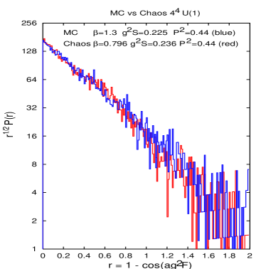
Figure 1: The distribution of plaquette values is well approximated by an inverse square root times an exponential decay law. This provides numerical evidence for the self-thermalization of the classical U(1) lattice system due to its chaotic dynamics (red histogram), as well as of the Monte-Carlo heat bath algorithm (blue histogram).

We now further demonstrate the validity of the relation (17) by showing the equivalence of the two theories for an important observable, the expectation value of the modulus squared of the Polyakov line on the respective periodic lattices. We note that this is the standard order parameter of the lattice gauge theory, which vanishes at strong coupling and is nonzero below a critical coupling $\beta_{c}\approx 1$, indicating the transition to the Coulomb phase. Figure 2 shows the Polyakov line modulus squared averaged over the 3-volume of the 4-dimensional lattice and over 20,000 quantum Monte-Carlo configurations (red squares) as a function of the average 4-dimensional lattice action per plaquette $\Sigma_{\rm P}=g^{2}S_{4}$.

On the same plot the same order parameter is shown (green dots) as a function of the expectation value of the lattice magnetic energy $\Sigma_{\rm P}=g^{2}aE_{\rm mag}$, per plaquette, of the classical configuration. The average here was calculated, after an additional brief Hamiltonian equilibration on the classical four-dimensional lattice, as an ergodic average by temporal sampling of a single evolving lattice field configuration. We note that these two sets of points follow the same scaling law.

The reason that we do not plot the modulus of the Polyakov line as a function of the inverse coupling $\beta$, as it is usually done, is that the classical Hamiltonian (18) does not contain such a coupling constant. Its solutions are solely characterized by the value of the total energy or, because of its ergodicity properties, by the average value of the magnetic energy. The fact that our simulation points obtained for the quantum field theory on the four-dimensional Euclidean lattice and the (4+1)-dimensional classical theory coincide when we impose the relation (17) constitutes the desired evidence. (One might consider relating the two results via the coupling constant $\beta_{5}$ used in the generation of the initial conditions for the classical field configuration. However, this would be inappropriate, because the five-dimensional lattice provides us solely with a convenient algorithm for generating randomized initial data. We could have started the classical calculation with an arbitrary initial configuration of the same total energy, without any reference to a five-dimensional lattice, and would have obtained the same results, albeit after much longer microcanonical equilibration.)

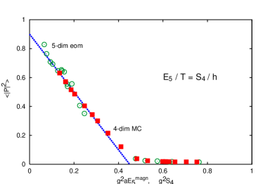
Figure 2: The order parameter, the absolute value square of the Polyakov line averaged over the lattice and over many configurations obtained by classical Hamiltonian dynamics is plotted against the magnetic energy of the four-dimensional spatial lattice (open circles), and the same quantity obtained by traditional quantum Monte-Carlo simulation on a Euclidean four-dimensional lattice against the four-dimensional action (filled boxes), respectively. These results coincide, if and only if $E_{5}/T=S_{4}/\hbar$.

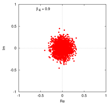
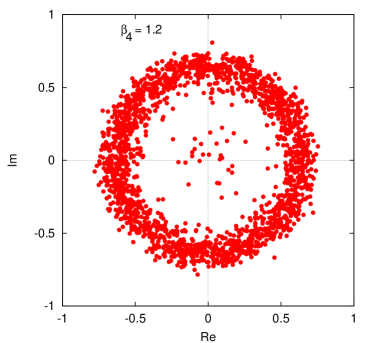
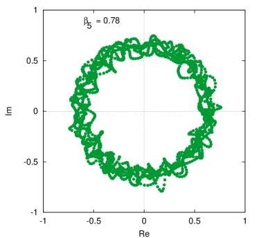
Figure 3: Complex Polyakov line values from 4-dimensional quantum Monte Carlo simulation (red dots) and from (4+1)-dimensional classical Hamiltonian equation of motion (green dots) at $aE_{4}^{mag}/T=S_{4}/\hbar$.

In order to further confirm the validity of the relation between the four-dimensional quantum and (4+1)-dimensional classical lattice U(1) theories it is illustrative to look at scatter plots of sampled values of the Polyakov line in the complex plane. In Figure 3 the results from the four-dimensional quantum Monte-Carlo simulation are shown as red dots, and the results from the (4+1)-dimensional classical Hamiltonian evolution for a single trajectory are represented by green dots. The correspondence in the four parts of Fig. 3 is again made by selecting pairs of simulations satisfying the relation (17). The overlap of the distributions is excellent, both for the modulus and the phase of the Polyakov line. Some initial points in the center of the rings for supercritical couplings $\beta_{4}=1/g_{4}^{2}\geq 1$ are artefacts from an initial heating phase in the quantum Monte Carlo simulations. They would be absent, if we had started the sampling process at a later time. In the classical Hamiltonian evolution the ergodic sampling was started also only after a transitory period, in which the electric and magnetic field energies equilibrated (in 4+1 dimensions, the ratio of electric and magnetic energy is 2:3, not 1:1 as in the usual (3+1)-dimensional case).

V Conclusion

In conclusion, we have demonstrated that the mechanism of chaotic quantization - conjectured earlier on the basis of non-Abelian gauge theories in 3 and 3+1 dimensions - also works for the compact Abelian lattice gauge theory in 4 and 4+1 dimensions. The correspondence between the classical and quantum gauge theories is given by the general formula $\hbar=aT$, which encodes physical properties of the higher dimensional theory into the Planck constant. Our result supports the speculation that chaotic quantization may be a physical mechanism for the quantization of (gauge) fields. This could make it eventually possible to construct a classical field theory encompassing both, gravity and the standard model of particle physics. In this framework, Planck’s constant $\hbar$ would become a parameter of the low-frequency, long-second-time limit of the fundamental classical field theory.

Finally we would like to address the question whether factorizing the Planck constant would be tantamount to the construction of a hidden variable theory. We believe that this is not the case, since none of the established rules of quantum physics are violated. The four-dimensional quantum field theory is given by a Euclidean functional integral, which is exactly the path integral that defines the vacuum sector of the compact U(1) gauge theory in (3+1) dimensions. The higher dimensional classical dynamics “acts” as a quantum field theory in four Euclidean dimensions.

Acknowledgments: This work was supported in part by DOE grant FG02-96ER-40945 and the Hungarian National Research Fund OTKA with the contract number T 034269.

Appendix A Chaotic quantization of harmonic oscillator

In order to help to gain a deeper insight into the chaotic quantization mechanism we present here a limiting case, the harmonic oscillator. Of course, pure lattice gauge theories cannot be used as models of the oscillator because they lead to massless particles in the continuum limit with a trivial dispersion relation $\omega=0$ in the $0+1$ dimensional case of ordinary quantum mechanics. An additional ingredient is needed for this purpose; we choose a complex scalar (Higgs) field which generates mass for the U(1) fields leading to the desired harmonic oscillator description in the low dimensional case. We consider the following action,

$$S=\int\left(-\frac{1}{4}F_{\mu\nu}F^{\mu\nu}+\frac{1}{2}|D_{\mu}\Phi|^{2}-V(|\Phi|)\right)d^{4}x$$ (29)

where the Higgs potential $V$ prefers a non-trivial vacuum state $|\Phi(t,x)|=R$. The Euclidean lattice version of this theory is investigated on a narrow, $N\times 1$ stripe in the $t-x$ plane (here $t$ denotes the ”ordinary” Euclidean time direction), having a periodic boundary condition in the dummy $x$ direction. The link phases starting at sites $t_{j}=ja$ and pointing in the (extremely short) $x$ direction are denoted by $\varphi_{j}$, the ones pointing in the $t$ direction by $p_{j}$. The complex fields at site positions are given by $\Phi(t_{j})=R_{j}e^{i\vartheta_{j}}$. The lattice action is decomposed as

$$S_{E,lat}\>=\>S_{g}+S_{x}+S_{t},$$ (30)

with

$$S_{g} = \frac{1}{g^{2}}\sum_{j}1-\cos(\varphi_{j+1}-\varphi_{j}),$$

$$S_{x} = \frac{a^{2}}{2}\sum_{j}R_{j}^{2}\left|e^{i(\varphi_{j}+\vartheta_{j})}-e^{i\vartheta_{j}}\right|^{2},$$

$$S_{t} = a^{2}\sum_{j}\left|R_{j+1}e^{i(\vartheta_{j+1}+p_{j})}-R_{j}e^{i\vartheta_{j}}\right|^{2}.$$ (31)

In the Higgs phase with a Lorentz-invariant (in the case of $0+1$ dimensional quantum mechanics, just simply static) modulus $R_{j}=R$, terms containing $\varphi_{j}$ decouple from the rest. This constitutes the lattice action for the harmonic oscillator, reducing the dynamics to that of a long chain of minimal plaquettes in the $t$ direction:

$$S_{lat}[\varphi]=\frac{1}{g^{2}}\sum_{j}(1-\cos(\varphi_{j+1}-\varphi_{j}))+(aR)^{2}\sum_{j}(1-\cos\varphi_{j}).$$ (32)

With the correspondence $\omega=gR$ and $\varphi_{j}=gq_{j}\,\sqrt{m/a}$ we get the familiar action of the harmonic oscillator in the small phase (either weak coupling, or small amplitude, or small oscillator mass) limit

$$S_{lat}[q]=a\sum_{j}\left(\frac{m}{2}\left(\frac{q_{j+1}-q_{j}}{a}\right)^{2}+\frac{m\omega^{2}}{2}q_{j}^{2}\right).$$ (33)

For $a\rightarrow 0$ this leads to the continuum Euclidean action of a single harmonic oscillator:

$$S_{c}[q]\>=\>\int\left(\frac{m}{2}\dot{q}^{2}+\frac{m\omega^{2}}{2}q^{2}\right)dt.$$ (34)

We now turn to the analysis of the Hamiltonian description of this lattice chain model (32) describing its classical evolution in a second time $s$. We use the Hamiltonian

$$H_{5}=\frac{a}{2g^{2}}\sum_{j}\left(\frac{d\varphi_{j}}{ds}\right)^{2}+\frac{1}{a}S_{lat}[\varphi].$$ (35)

The classical equation of motion, presented in a scaled time variable $s/a$ becomes

$$\frac{d^{2}\varphi_{j}}{d(s/a)^{2}}=\sin(\varphi_{j+1}-\varphi_{j})-\sin(\varphi_{j}-\varphi_{j-1})-(a\omega)^{2}\sin\varphi_{j}.$$ (36)

The only parameter in this $s$-dynamics is the scaled frequency $G=a\omega$. In a molecular field approximation each link phase (or plaquette phase) would behave like a pendulum with a harmonically perturbed pivot point. Such systems are known to be chaotic PEND-TO-CHAOS .

In order to understand how the classical chaotic mechanics leads to a distribution in the second time $s$, which resembles that distribution applied in Euclidean quantum field theory, the key property is the relation between the equations of motion and a Fokker-Planck-Kolmogorov equation. This relation has also been studied at length in chaotic dynamics and the circumstances when the chaotic motion can be replaced by a diffusion in phase space governed by a Fokker-Planck type equation have been investigated. Here we follow a presentation given in Chapter 6 of Ref.PEND-TO-CHAOS .

First the differential equations are solved in discrete time steps, $\Delta s$, generating a mapping in the phase space:

$$\overline{q_{i}} = q_{j}+\frac{p_{j}}{m}\Delta s,$$

$$\overline{p_{i}} = p_{j}+F_{j}\Delta s$$ (37)

with the following force in the lattice chain model

$$F_{j}=-\frac{g}{a}\sqrt{\frac{m}{a}}\frac{\partial}{\partial\varphi_{j}}S_{lat}.$$ (38)

The mapping should be in action-angle variables; the lattice model is readily formulated in terms of the angles $\varphi_{j}$. The corresponding scaled action variable we denote by $I_{j}=a(d\varphi_{j}/ds)$. The (2-time) Hamiltonian contains the following kinetic energy term

$$H_{5}^{kin}=\frac{m}{2}\sum_{i}\left(\frac{dq_{i}}{ds}\right)^{2}=\frac{1}{g^{2}a}\frac{1}{2}\sum_{i}I_{i}^{2}.$$ (39)

allowing us to write the mapping in dimensionless action – angle variables as follows

$$\overline{\varphi_{j}} = \varphi_{j}+\frac{\Delta s}{a}I_{j},$$

$$\overline{I_{j}} = I_{j}-\frac{\Delta s}{a}g^{2}\frac{\partial}{\partial\varphi_{j}}S_{lat}.$$ (40)

An equivalent Fokker-Planck-Kolmogorov equation is then valid for the distribution of $I_{i}$ in a long-term sampling of phase space trajectory:

$$\frac{\partial{\cal F}}{\partial s}=-\frac{\partial}{\partial I_{i}}(A_{i}{\cal F})+\frac{1}{2}\frac{\partial}{\partial I_{i}}\frac{\partial}{\partial I_{j}}(B_{ij}{\cal F})$$ (41)

with the following drift and diffusion coefficients

$$A_{i} = \frac{a}{\Delta s}\langle\langle\overline{I}_{i}-I_{i}\rangle\rangle,$$

$$B_{ij} = \frac{a}{\Delta s}\langle\langle(\overline{I}_{i}-I_{i})(\overline{I}_{j}-I_{j})\rangle\rangle$$ (42)

Here the averaging over different observation moments $s$ and different trajectories (wherever started) can be replaced by an average over the angle variables. This is a central statement of chaotic dynamics, giving a statistical physics perspective to deterministic dynamical systems. This is as well the key mechanism beyond the chaotic quantization, arriving at a Fokker-Planck correspondence, which used to be the starting point of the stochastic quantization method.

For our lattice oscillator model we get $A_{i}=0$ and

$$B_{ij}=\frac{\Delta s}{a}\left((1+\frac{(a\omega)^{2}}{2})\delta_{ij}-\frac{1}{2}(\delta_{i-1,j}+\delta_{i+1,j})\right).$$ (43)

meaning that the diffusion matrix, the coefficient of the scaled time-step $\Delta s/a$ in the matrix $B_{ij}$ is readily recognized as the the harmonic oscillator matrix in the quantum mechanical Euclidean path integral formalism.

At this point we still seek to determine the long second-time limit of the diffusion matrix $B_{ij}$. This can be understood with the help of the Green-Kubo formula Dorfman which connects the microscopical dynamics with the linear response approximation. The diffusion-like Fokker-Planck equation is actually the leading order cumulant expansion to the more general case, the Fourier transform of the probability is taken in the infrared limit associated to the basic action variables:

$${\cal F}_{k}=\left\langle e^{ik_{j}\Delta I_{j}}\right\rangle\approx\exp\left(-k_{i}\langle\Delta I_{i}\Delta I_{j}\rangle k_{j}\right).$$ (44)

Back Fourier transformation leads then to the second derivative according to the $I_{j}$ variables; the first derivative (drift) term vanishes for time reversal dynamics, such as governed by conservative Hamiltonians. The diffusion coefficient in scaled time $s/a$ becomes

$$B_{ij}=\left\langle a\frac{\Delta I_{i}}{\Delta s}\Delta I_{j}\right\rangle=\int_{0}^{s/a}\langle\dot{I}_{i}(s)\dot{I}_{j}(s^{\prime})\rangle ds^{\prime}.$$ (45)

Assuming now that the correlation of the action variables depends only on the absolut value of second-time difference, as it is the case both in stochastic and chaotic processes, we arrive at

$$B_{ij}=\int_{0}^{s/a}\langle\dot{I}_{i}(s^{\prime})\dot{I}_{j}(0)\rangle ds^{\prime}.$$ (46)

The characteristic correlation of the force ($\dot{I}$) is an exponential decay both in the stochastic, as well as in the chaotic quantization. In the former case a Langevin equation with white noise leads to forgetting, in the latter case the instability of nearby trajectories expressed by positive Lyapunov exponents. The general behavior is then

$$\langle\dot{I}_{i}(s^{\prime})\dot{I}_{j}(0)\rangle=e^{-\gamma s^{\prime}}\langle\dot{I}_{i}(0)\dot{I}_{j}(0)\rangle.$$ (47)

The second-time integral in (46) can now be analytically done leaving us with

$$B_{ij}=\frac{1-e^{\gamma s}}{a\gamma}$$ (48)

For a short s-time evolution it gives back the result of (43), in the long term, however, leads to a constant times the matrix describing the oscillator’s path integral in ordinary quantum mechanics:

$$\lim_{s\rightarrow\infty}B_{ij}=\frac{1}{a\gamma}\left((1+\frac{(a\omega)^{2}}{2})\delta_{ij}-\frac{1}{2}(\delta_{i-1,j}+\delta_{i+1,j})\right).$$ (49)

This proves our conjecture for the harmonic oscillator, without extended numerical simulations.

Finally some remarks are in order to explain how dimensionful scales and parameters enter in the interpretation of lattice model results. Of course, both the familiar quantum Monte Carlo and the second-time Hamiltonian equation of motion (shortly EOM) method deals with scaled quantities on the lattice (and with a scaled time) not having any length (fm) or energy (MeV) dimensions. Besides the lattice spacing $a$, giving the unit of length, either the unit of quantum action, $\hbar\approx 197$ MeVfm is given, or in the EOM method instead of $\hbar$ an energy, which is conserved in total, is given.

The study of the diffusion coefficient in phase space describes the chaotic evolution in mid terms, the elapsed second time $\Delta s$ to be taken between an autocorrelation time $s_{c}$ when initial phase points are remembered by the evolution trajectory (there is an exponential forgetting of nearbyness of the initial conditions set by the leading Lyapunov exponent) and the longer time when equipartition completes. As in the case of simple Brownian motion, the kinetic energy starts to grow linearly for short time $s$ but levels off at an equipartition value, in our case we have

$$\langle\frac{1}{2g^{2}a}\sum_{i}I_{i}^{2}\rangle=N\frac{T}{2}(1-e^{-\gamma s})\rightarrow NT/2,$$ (50)

where $N$ is the ordinary time extension of the path integral lattice. (This is the correct scaling of Brownian motion parameters with ”volume”.) Expressing the product of the equipartition temperature $T$ and the inverse equipartition time $\gamma$ in a lattice scaled fashion we arrive at

$$aT=\frac{1}{g^{2}N}\sum_{i}B_{ii}.$$ (51)

containing the average eigenvalue of the diffusion matrix. On the other hand the long time equipartition reaches

$$\langle\frac{1}{2g^{2}a}\sum_{i}I_{i}^{2}\rangle\rightarrow\frac{1}{2}TN,$$

$$\langle\frac{1}{a}S_{lat}\rangle\rightarrow\frac{1}{2}TN,$$ (52)

while the distribution ${\cal F}$ approaches the canonical one

$${\cal F}\propto e^{-N}=e^{-\langle H_{5}\rangle/T}=e^{-2\langle S_{lat}/(aT)\rangle}$$ (53)

This canonical distribution is eventually interpreted as the Euclidean quantum wave function, ${\cal F}\sim\exp(-S/\hbar)$, (continuing back to real time it would be $\exp(iS/\hbar)$ constituting the solution of the Schrödinger equation). This interpretation of the chaotic distribution allows us to connect the Planck constant experienced in the 1-time quantum mechanics with parameters of the phase space diffusion of the 2-time Hamiltonian:

$$\hbar=\frac{1}{2}aT=\frac{1}{2g^{2}}\frac{1}{a\gamma}\overline{\lambda}(B).$$ (54)

For the oscillator in the $N\rightarrow\infty$ limit the average eigenvalue becomes $\overline{\lambda}(B)=(2+(a\omega)^{2})$ leading to

$$\hbar=\frac{1}{g^{2}}\frac{1}{a\gamma}\left(1+\frac{(a\omega)^{2}}{2}\right)$$ (55)

or with $a\rightarrow 0$ at finite $g$ and $\omega=gR$ values, the same value as for free fields,

$$\hbar=\frac{1}{g^{2}}\,\frac{1}{\gamma a}.$$ (56)

relating Planck’s constant with the leading Lyapunov exponent of the chaotic dynamics in s-time.

For the classical simulation input is the scaled energy, $g^{2}aE_{5}$ which is conserved, and the lattice size $N$. For the quantum MC simulation input is $\beta=1/(g^{2}\hbar)$ and the size $N$. From the above equipartition by chaotic dynamics we got $g^{2}\hbar=1/(a\gamma)=g^{2}aE_{5}/(2N)$. Since by construction the half of $E_{5}$ is $S_{4}/a$ at equipartition, we tend to a final state where $\langle S_{lat}\rangle\>=\>N\hbar$ . As we equipartition energy in $5d$, making a temperature $T$, with proper scaling we create an action in $4d$ with an $\hbar$ value per degree of freedom. In this sense the value of $\hbar$ is determined by the scaled total energy per degree of freedom into the classical EOM simulation. Its interpretation and descendence are, however, quite untraditional in chaotic quantization.

References

- (1) S. G. Matinyan, G. K. Savvidy, N. G. Ter-Arutyunyan-Savvidy: Sov. Phys. JETP 53, 421 (1981).
- (2) T. S. Biró, S. G. Matinyan, B. Müller, Chaos and Gauge Field Theory (World Scientific, Singapore 1994).
- (3) B. Müller, A. Trayanov, Phys. Rev. Lett. 68, 3387 (1992); C. Gong, Phys. Rev. D 49, 2642 (1994); J. Bolte, B. Müller, A. Schäfer, Phys. Rev. D 61, 054506 (2000).
- (4) T. S. Biró, S. G. Matinyan, B. Müller, Found. Phys. Lett. 14, 471 (2001); arXiv:hep-th/9908031, arXiv:hep-th/0301131.
- (5) C. Beck, Nonlinearity 8, 423 (1995).
- (6) see e. g. J. R. Dorfman, An Introduction to Chaos in Nonequilibrium Statistical Mechanics, Cambridge Lecture Notes in Physics 14 (Cambridge University Press, Cambridge, 1999).
- (7) G. ’t Hooft: Class. Quant. Grav. 16, 3283 (1999); arXiv:hep-th/0003004, arXiv:hep-th/0104219, arXiv:hep-th/0104080.
- (8) G. Parisi, Y. S. Wu, Sci. Sin. 24, 483 (1981).
- (9) H. Markum, R. Pullirsch, W. Sakuler, arXiv:hep-lat/0205003, arXiv:hep-lat/0209039; B. M. Gripaios, Phys. Rev. D 67, 025023 (2003); T. S. Biró, H. Markum, R. Pullirsch, W. Sakuler, arXiv:hep-lat/0210020.
- (10) T. S. Biró, C. Gong, B. Müller, A. Trayanov, Int. J. Mod. Phys. C 5, 113 (1994).
- (11) R. Z. Sagdeev, D. A. Usikov, G. M. Zaslavsky, Nonlinear Physics: From the Pendulum to Turbulence and Chaos, (Harwood Academic Publishers, Chur, Switzerland, 1988).
- (12) S. G. Matinyan, Y. J. Ng, J.Phys.A: Math.Gen. 36, L417, 2003 and references therein.