Meson and Baryon Spectroscopy on a Lattice.

Abstract

I review the results of hadron spectroscopy calculations from lattice QCD for an intended audience of low energy hadronic physicists. I briefly introduce the ideas of numerical lattice QCD. The various systematic errors, such as the lattice spacing and volume dependence, in lattice QCD calculations are discussed. In addition to the discussion of the properties of ground state hadrons, I also review the small amount of work done on the spectroscopy of excited hadrons and the effect of electromagnetic fields on hadron masses. I also discuss the attempts to understand the physical mechanisms behind hadron mass splittings.

1 INTRODUCTION

QCD at low energies is hard to solve, perhaps too hard for mere mortals to solve, even when assisted with the latest supercomputers. QCD is the theory that describes the interactions of quarks and gluons. QCD has been well tested in high energy scattering experiments where perturbation theory is valid. However, QCD should also describe nuclear physics and the mass spectrum of hadrons. Hadron masses depend on the coupling ($g$) like $M\sim e^{-1/g^{2}}$ hence perturbation theory can’t be used to compute the masses of hadrons such as the proton.

The only technique that offers any prospect of computing masses and matrix elements non-perturbatively, from first principles, is lattice QCD. In lattice QCD, QCD is transcribed to a lattice and the resulting equations are solved numerically on a computer. The computation of the hadron spectrum using lattice QCD started in the early 80’s [1, 2]. The modern era in lattice QCD calculations of the hadron spectrum started with the results of the GF11 group [3, 4]. The GF11 group were the first to try to quantify the systematic errors in taking the continuum and infinite volume limits.

The goal of a “numerical solution” to QCD is not some kind of weird and misguided reductionist quest. Our inability to solve QCD has many profound consequences. A major goal of particle physics is to look for evidence for physics beyond the standard model of particle physics. One way of doing this is to extract the basic parameters of the standard model and look for relations between them that suggest deeper structure. To test the quark sector of the standard model requires that matrix elements are computed from QCD [5]. The problem of solving QCD is symbolically summarised by the errors on the quark masses. For example, the allowed range on the strange quark mass in the particle data table [6] is 80 to 155 MeV; a range of almost 100%. The value of top quark mass, quoted in the particle data table, is $174.3\pm 5.1$ GeV As the mass of the quark increases its relative error decreases. The dynamics of QCD becomes simpler as the mass of the quarks gets heavier. Wittig has reviewed the latest results for the light quark masses from lattice QCD [7] Irrespective of applications of solutions to QCD to searches for physics beyond the standard model, QCD is a fascinating theory in its own right. QCD does allow us to test our meagre tools for extracting non-perturbative physics from a field theory.

In this review I will focus on the results from lattice gauge theory for the masses of the light mesons and baryons. I will not discuss flavour singlet mesons as these have been reviewed by Michael [8, 9]. There has been much work on the spectroscopy of hadrons that include heavy quarks [10, 11, 12], however I will not discuss this work. The treatment of heavy quarks (charm and bottom) on the lattice has a different set of problems and opportunities over those for light quarks. Although the spectroscopy of hadrons with heavy quarks in them can naturally be reviewed separately from light quark spectroscopy, the physics of heavy hadrons does depend on the light quarks in the sea. In particular the hyperfine splittings are known to have an important dependence on the sea quarks [12].

Until recently, the computation of the light hadron spectrum used to be just a test of the calculational tools of lattice QCD. The light hadron spectrum was only really good for providing the quark masses and estimates of the systematic errors. However, the experimental program at places such as the Jefferson lab [13, 14, 15] has asked for a new set of quantities from lattice QCD. In particular the computation of the spectrum of the $N^{\star}$’s is now a goal of lattice QCD calculations.

As the aim of the review is to focus more on the results of lattice calculations, I shall mostly treat lattice calculations as a black box that produces physical numbers. However, “errors are the kings” of lattice QCD calculations because the quality and usefulness of a result usually depends on the size of its error bar, hence I will discuss the systematic errors in lattice calculations. Most of systematic errors in lattice QCD calculations can be understood using standard field theory techniques. I have also included an appendix A. on some of the “technical tricks” that are important for lattice QCD insiders, but of limited interest to consumers of lattice results. However, it is useful to know some of the jargon and issues, as they do effect the quality of the final results.

There are a number of text books on lattice QCD. For example the books by Montvay and Munster [16], Rothe [17], Smit [18] and Creutz [19] provide important background information. The large review articles by Gupta [20], Davies [11] and Kronfeld [21] also contain pertinent information. The annual lattice conference is a snap-shot of what is happening in the lattice field every year. The contents of the proceedings of the lattice conference have been put on the hep-lat archive for the past couple of years [22, 23, 24]. The reviews of the baryon spectroscopy from lattice QCD by Bali [25] and Edwards [26] describe a different perspective on the field to mine. There used to be a plenary reviews specifically on hadron spectroscopy at the lattice conference [27, 28, 29, 30, 31]. The subject of hadron spectroscopy has now been split into a number of smaller topics, such as quark masses.

If the reader wants to play a bit with some lattice QCD code, then the papers by Di Pierro [32, 33, 34], contain some exercises and pointers to source code. The MILC collaboration also make their code publicly available (try putting “MILC collaboration” into a search engine).

2 BASIC LATTICE GAUGE THEORY

In this section, I briefly describe the main elements of numerical lattice QCD calculations. Quantum Chromodynamics (QCD) is the quantum field theory that describes the interactions of elementary particles called quarks and gluons. The key aspect of a quantum field theory is the creation and destruction of particles. This type of dynamics is crucial to QCD and one of the reasons that it is a hard theory to solve.

In principle, because we know the Lagrangian for QCD, the quantum field theory formalism should allow us to compute any quantity. The best starting point for solving QCD on the computer is the path integral formalism. The problem of computing bound state properties from QCD is reduced to evaluating equation 1.

$$\langle B\rangle = \frac{1}{{\cal Z}}\int dU\int d\psi\int d\overline{\psi}\;Be^{-S_{F}-S_{G}}$$ (1)

$${\cal Z} = \int dU\int d\psi\int d\overline{\psi}e^{-S_{F}-S_{G}}$$ (2)

where $S_{F}$ and $S_{G}$ are the actions for the fermion and gauge fields respectively. The path integral is defined in Euclidean space for the convergence of the measure.

The fields in equation 1 fluctuate on all distance scales. The short distance fluctuations need to be regulated. For computations of non-perturbative quantities a lattice is introduced with a lattice spacing that regulates short distance fluctuations. The lattice regulator is useful both for numerical calculations, as well for formal work [35] (theorem proving), because it provides a specific representation of the path integral 1.

A four dimensional grid of space-time points is introduced. A typical size in lattice QCD calculations is $24^{3}\;48$. The introduction of a hyper-cubic lattice breaks Lorentz invariance, however this is restored as the continuum limit is taken. The lattice actions do have a well defined hyper-cubic symmetry group [36, 37]. The continuum QCD Lagrangian is transcribed to the lattice using “clever” finite difference techniques.

In the standard lattice QCD formulation, the decision has been made to keep gauge invariance explicit. The quark fields are put on the sites of the lattice. The gauge fields connect adjacent lattice points. The connection between the gauge fields in lattice QCD and the fields used in perturbative calculations is made via:

$$U_{\mu}(x)=e^{-giA_{\mu}(x)}$$ (3)

The gauge invariant objects are either products of gauge links between quark and anti-quark fields, or products of gauge links that form closed paths. All gauge invariant operators in numerical lattice QCD calculations are built out of such objects. For example the lattice version of the gauge action is constructed from simple products of links called plaquettes.

$$U_{P}(x;\mu\nu)=U_{\mu}(x)U_{\nu}(x+\hat{\mu})U_{\mu}(x+\hat{\nu})^{\dagger}U_{\nu}(x)^{\dagger}$$ (4)

The Wilson gauge action

$$S_{G}=-\beta(\sum_{p}\frac{1}{2N_{c}}\mbox{Tr}(U_{P}+U_{P}^{\dagger})-1)$$ (5)

is written in terms of plaquettes. $N_{c}$ is the number of colours. The action in 5 can be expanded in the lattice spacing using equation 3, to get the continuum gauge action.

$$S_{G}=a^{4}\frac{\beta}{4N_{c}}\sum_{x}\mbox{Tr}(F_{\mu\nu}F^{\mu\nu})+O(a^{6})$$ (6)

The coupling is related to $\beta$ via

$$\beta=\frac{2N_{c}}{g^{2}}$$ (7)

The coupling in equation 7 is known as the bare coupling. More physical definitions of the coupling [38] are typically used in perturbative calculations.

The fermion action is generically written as

$$S_{F}=\overline{\psi}M\psi$$ (8)

where $M$ is called the fermion operator, a lattice approximation to the Dirac operator.

One approximation to the fermion operator on the lattice is the Wilson operator. There are many new lattice fermion actions, however the basic ideas can still be seen from the Wilson fermion operator.

$$S_{f}^{W}=\sum_{x}(\kappa\sum_{\mu}\{\overline{\psi}_{x}(\gamma_{\mu}-1)U_{\mu}(x)\psi_{x+\mu}-\overline{\psi}_{x+\mu}(\gamma_{\mu}+1)U_{\mu}^{\dagger}(x)\psi_{x}\}+\overline{\psi}_{x}\psi_{x})$$ (9)

The Wilson action can be expanded in the lattice spacing to obtain the continuum Dirac action with lattice spacing corrections. to the Dirac Lagrangian. The $\kappa$ parameter is called the hopping parameter. It is a simple rescaling factor that is related to the quark mass via

$$\kappa=\frac{1}{2(4+m)}$$ (10)

at tree level. An expansion in $\kappa$ is not useful for light quarks, because of problems with convergence, however for a few specialised applications, it is convenient to expand in terms of $\kappa$ [39]. The fermion operator in equation 9 contains a term called the Wilson term that is required to remove fermion doubling [16, 17, 18]. The Wilson term explicitly breaks chiral symmetry so equation 10 gets renormalised. Currently, there is a lot of research effort in designing lattice QCD actions for fermions with better theoretical properties. I briefly describe some of these developments in the appendix A.

Most lattice QCD calculations obtain hadron masses from the time sliced correlator $c(t)$.

$$c(t)=\langle\sum_{\underline{x}}e^{ipx}O(\underline{x},t)O(0,0)^{\dagger}\rangle$$ (11)

where the average is defined in equation 1.

Any gauge invariant combination of quark fields and gauge links can be used as interpolating operators ($O(\underline{x},t)$) in equation 11. An example for an interpolating operator in equation 11 for the $\rho$ meson would be

$$O(\underline{x},t)_{i}=\overline{\psi_{1}}(\underline{x},t))\gamma_{i}\psi_{2}(\underline{x},t))$$ (12)

The interpolating operator in equation 12 has the same $J^{PC}$ quantum numbers as the $\rho$.

The operator in equation 12 is local, as the quark and anti-quarks are at the same location. It has been found to better to use operators that build in some kind of “wave function” between the quark and anti-quarks. In lattice-QCD-speak we talk about “smearing” the operator. An extended operator such as

$$O(\underline{x},0)=\sum_{\underline{r}}f(\underline{r})\overline{\psi}_{1}(\underline{x},0))\gamma_{i}\psi_{2}(\underline{x}+\underline{r},0))$$ (13)

might have a better overlap to the $\rho$ meson than the local operator in equation 13. The $f(\underline{r})$ function is a wave-function like function. The function $f$ is designed to give a better signal, but the final results should be independent of the choice of $f$. Typical choices for $f$ might be hydrogenic wave functions. Unfortunately equation 13 is not gauge invariant, hence vanishes by Elitzur’s theorem [40]. One way to use an operator such as equation 13 is to fix the gauge. A popular choice for spectroscopy calculations is Coulomb’s gauge. On the lattice Coulomb’s gauge is implemented by maximising

$$F=\sum_{x}\sum_{i=\hat{x}}^{\hat{z}}(U_{i}(x)+U_{i}^{\dagger}(x))$$ (14)

The gauge fixing conditions that are typically used in lattice QCD spectroscopy calculations are either: Coulomb or Landau gauge. Different gauges are used in other types of lattice calculations.

Non-local operators can be measured in lattice QCD calculations,

$$O(\underline{x},0)=\sum_{\underline{r}}\overline{\psi}_{1}(\underline{x},0))\gamma_{i}\psi_{2}(\underline{x}+\underline{r},0))$$ (15)

however these do not have any use in phenomenology [41, 42, 43, 44, 45], because experiments are usually not sensitive to single $\overline{\psi}\psi$ Fock states.

There are also gauge invariant non-local operators that are used in calculations.

$$O(\underline{x},t)=\overline{\psi}_{1}(\underline{x},t)\gamma_{i}F(\underline{x},\underline{x}+\underline{r})\psi_{2}(\underline{x}+\underline{r},t)$$ (16)

where $F(\underline{x},\underline{x}+\underline{r})$ is a product of gauge links between the quark and anti-quark.

There are many different paths between the quark and anti-quark. It has been found useful to fuzz [46]. the gauge links by adding bended paths:

$$U_{new}=P_{SU(3)}(cU_{old}+\sum_{1}^{4}U_{u-bend})$$ (17)

where $P_{SU(3)}$ projects onto SU(3). There are other techniques for building up gauge fields between the quark and anti-quark fields, based on computing a scalar propagator [47, 48].

The path integral in equation 1 is evaluated using algorithms that are generalisations of the Monte Carlo methods used to compute low dimensional integrals [49]. The physical picture for equation 11 is that a hadron is created at time 0, from where it propagates to the time t, where it is destroyed. This is shown in figure 1. Equation  11 can be thought of as a meson propagator. Duncan et al. [50] have used the meson propagator representation to extract couplings in a chiral Lagrangian.

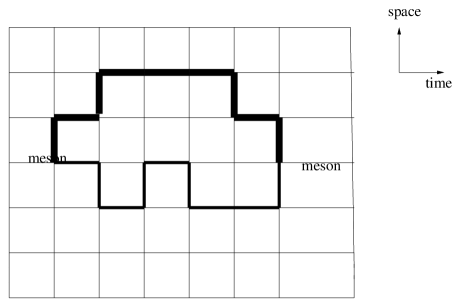
Figure 1: Physical picture of a meson propagator on the lattice. The thick lines are the quark propagators.

The algorithms, usually based on importance sampling, produce $N$ samples of the gauge fields on the lattice. Each gauge field is a snapshot of the vacuum. The QCD vacuum is a complicated structure. There is a community of people who are trying to describe the QCD vacuum in terms of objects such as a liquid of instantons (for example [51]). The lattice QCD community are starting to create publicly available gauge configurations [52, 53]. This is particularly important due to the high computational cost of unquenched calculations. An archive of gauge configurations has been running at NERSC for many years.

The correlator $c(t)$ is a function of the light quark propagators ($M(U(i))_{q}^{-1}$) averaged over the samples of the gauge fields.

$$c(t)\sim\frac{1}{N}\sum_{i}^{N}f(M(U(i))^{-1},M(U(i))^{-1})$$ (18)

The quark propagator $M^{-1}$ is the inverse of the fermion operator. The quark propagator depends on the gauge configurations from the gauge field dependence of the fermion action (see 9 for example).

The correlator in equation 18 is essentially computed in two stages. First the samples of the gauge configurations are generated. These are the building blocks of most lattice QCD calculations. The correlators for specific processes are computed by calculating the hadron correlator for each gauge configuration and then averaging over each gauge configuration.

To better explain the idea behind computing quark propagators in lattice QCD calculations, it is helpful to consider the computation of the propagator in perturbation theory. The starting point of perturbative calculations is when the quarks do not interact with gluons. This corresponds to quarks moving in gauge potentials that are gauge transforms from the unit configuration

$$A_{\mu}(x)=0\Rightarrow U_{\mu}(x)=1$$ (19)

Under these conditions the quark propagator can be computed analytically from the fermion operator using Fourier transforms (see  [17] for derivation).

$$M^{unit}=\frac{1}{\sum_{i=0}^{4}\gamma_{\mu}\sin(p_{\mu})+M(p)}$$ (20)

$$M(p)=m+\frac{2}{a}\sum_{\mu}sin^{2}(ap_{\mu}/1)$$ (21)

Although in principle the propagator in equation 20 could be used as a basis of a perturbative expansion of equation 18, the physical masses depend on the coupling like $M\sim e^{-1/g^{2}}$ (see section 3.2), so hadron masses can not be computed using this approach. The quark propagator on its own is not gauge invariant. Quark propagators are typically built into gauge invariant hadron operators. However, in a fixed gauge quark propagators can be computed and studied. This is useful for the attempts to calculate hadron spectroscopy using Dyson-Schwinger equations [54, 55].

In lattice QCD calculations the gauge fields have complicated space-time dependence so the quark propagator is inverted numerically using variants of the conjugate gradient algorithms [56]. Weak coupling perturbation theory on the lattice is important for determining weak matrix elements, quark masses and the strong coupling.

The sum over $\underline{x}$ in the time slice correlator (equation 11) projects onto a specific momentum at the sink. Traditionally for computational reasons, the spatial origin had to be fixed either at a point, or with a specific wave function distribution between the quarks. Physically, it would be clearly better to project out onto a specific momentum at the origin. The number of spatial positions at the origin is related to the cost of the calculation. There are new lattice techniques called “all-to-all” that can be used to compute a quark propagator from any point to another without spending prohibitive amounts of computer time [57, 58, 59].

There have been some studies of the point to point correlator [60, 61, 62]

$$\langle O(\underline{x},t)O(0,0)^{\dagger}\rangle$$ (22)

It was pointed out by Shuryak [63] that the correlator in equation 22 may be more easily compared to experiment. Also, the correlator 22 could give some information on the density of states. In practise the point to point correlators were quite noisy.

The physics from the time sliced correlator is extracted using a fit model [16]:

$$c(t)=a_{0}exp(-m_{0}t)+a_{1}exp(-m_{1}t)+\cdots$$ (23)

where $m_{0}$ ($m_{1}$) is the ground (first excited) state mass and the dots represent higher excitations. There are simple corrections to equation 23 for the finite size of the lattice in the time direction. In practise as recently emphasised by Lepage et al. [64], fitting masses from equation 23 is nontrivial. The fit region in time has to be selected as well as the number of exponentials. The situation is roughly analogous to the choice of “cuts” in experimental particle physics. The correlators are correlated in time, hence a correlated $\chi^{2}$ should be minimised. With limited statistics it can be hard to estimate the underlying covariance matrix making the $\chi^{2}/dof$ test nontrivial [65, 66]. As ensemble sizes have increased the problems resulting from poorly estimated covariance matrices have decreased.

It is usually better to measure a matrix of correlators so that variational techniques can be used to extract the masses and amplitudes [67, 68, 48].

$$c(t)_{A\;B}=\langle\sum_{\underline{x}}e^{ipx}O(\underline{x},t)_{A}O(0,0)_{B}^{\dagger}\rangle$$ (24)

The correlator in equation 24 is analysed using the fit model in equation 25.

$$c(t)_{A\;B}=\sum_{N=1..N_{0}}X_{A\;N}e^{-m_{N}}X_{N\;A}$$ (25)

The matrix $X$ is independent of time and in general has no special structure. The masses can be extracted from equation 25 either by fitting or by reorganising the problem as a generalised eigenvalue problem [69]. Obtaining the matrix structure on the right hand of equation 25 is a non-trivial test of the multi-exponential fit. One piece of “folk wisdom” is that the largest mass extracted from the fit is some average over the truncated states, and hence is unphysical. This may explain why the excited state masses obtained from [48] in calculation with only two basis states were higher than any physical state

The main (minor) disadvantage of variational techniques is that they require more computer time, because additional quark propagators have to be computed, if the basis functions are “smearing functions”. If different local interpolating operators are used as basis states, as is done for studies of the Roper resonance (see section 7.1), then there is no additional cost. The amount of computer time depends linearly on the number of basis states. Also the basis states have to be “significantly” different to gain any benefit. Apart from a few specialised applications [70] the efficacy of a basis state is not obvious until the calculations is done.

Although in principle excited state masses can be extracted from a multiple exponential fit, in practise this is a numerically non-trivial task, because of the noise in the data from the calculation. There is a physical argument [71, 72] that explains the signal to noise ratio. The variance of the correlator in equation 11 is:

$$\sigma_{O}^{2}=\frac{1}{N}(\langle(O(t)O(0))^{2}\rangle-c(t)^{2}$$ (26)

The square of the operator will couple to two (three) pion for a meson (baryon). Hence the noise to signal ratio for mesons is

$$\frac{\sigma_{M}(t)}{c(t)}\sim e^{(m_{M}-m_{\pi})t}$$ (27)

and noise to signal ratio for baryons is

$$\frac{\sigma_{B}(t)}{c(t)}\sim e^{(m_{B}-3/2m_{\pi})t}$$ (28)

The signal to noise ratio will get worse as the mass of the hadron increases.

In figure 2 I show some data for a proton correlator. The traditional way to plot a correlator is to use the effective mass plot.

$$m_{eff}=\log(\frac{c(t)}{c(t+1)})$$ (29)

When only the first term in equation 23 dominates, then equation 29 is a constant. There is a simple generalisation of equation 29 for periodic boundary conditions in time.

In the past the strategy used to be fit far enough out in time so that only one exponential contributed to equation 23. One disadvantage of doing this is that the noise increases at larger times, hence the errors on the final physical parameters become larger [64].

Many of the most interesting questions in hadronic physics involve the hadrons that are not the ground state with a given set of quantum numbers, hence novel techniques that can extract masses of excited states are very important.

Figure 2: Effective mass plot for proton correlators. Unquenched data from UKQCD [73] with $\kappa$=0.1350 , $\beta$ = 5.2.

Recently, there has been a new set of tools developed to extract physical parameters from the correlator $c(t)$ in equation 23. The new techniques are all based on the spectral representation of the correlator in equation 11.

$$c(t)=\int_{0}^{\infty}\rho(s)e^{-st}ds$$ (30)

The fit model in equation 23 corresponds to a spectral density of

$$\rho(s)=a_{0}\delta(s-m_{0})+a_{1}\delta(s-m_{1})$$ (31)

Spectral densities are rarely a sum of poles, except when the particles can’t decay such as in the $N_{c}\rightarrow\infty$ limit. Shifman reviews some of the physics in the spectral density [74]. As the energy increases it is more realistic to represent the spectral function as a continuous function. Leinweber investigated a sum rule inspired approach to studying hadron correlators [75] on the lattice. Allton and Capitani [76] generalised the sum rule analysis to mesons. The sum rule inspired spectral density is

$$\rho(s)=\frac{Z}{2M}\delta(s-M)+\theta(s-s_{0})\rho^{OPE}(s)$$ (32)

The operator product expansion is used to obtain the spectral density.

$$\rho^{OPE}(s)=\sum_{n=1}^{n_{0}}\frac{s^{n-1}}{(n-1)!}.C_{n}O_{n}(m_{q},\langle:\overline{q}q:\rangle)$$ (33)

where $m_{q}$ is the quark mass and $:\overline{q}q:$ is the quark condensate. The $C_{n}$ factors in equation  33 are obtained by putting the OPE expression for the quark propagator in 11. The final functions that are fit to the lattice data involve exponentials multiplied by polynomials in $1/t$ (where $t$ is the time). These kind of methods can also help to understand some of the systematic errors in sum rule calculations [75]. This hybrid lattice sum rule analysis is not in wide use in the lattice community. See [77] for recent developments. There has been an interesting calculation of the mass of the charm quark using sum rule ideas and lattice QCD data [78].

There is currently a lot of research into using the maximum entropy method to extract masses from lattice QCD calculations. Here I follow the description of the method used by CP-PACS [79]. There are other variants of the maximum entropy method in use. The maximum entropy approach [80] is based on Bayes theorem.

$$P(F\mid DH)\propto P(D\mid FH)P(F\mid H)$$ (34)

In equation 34 $F$ is the spectral function, $D$ is the data, and $H$ is the prior information such as $f(w)>0$, and $P(F\mid DH)$ is the conditional probability of getting $F$ given the data $D$ and priors $H$. The replacement of the fit model in equation 23 is

$$c_{f}(t)=\int_{0}^{\infty}K(w,t)f(w)dw$$ (35)

where the kernel $K$ is defined by

$$K(w,t)=e^{-wt}+e^{-w(T-t))}$$ (36)

with $T$ the number of time slices in the time direction.

$$P(D\mid FH) = \frac{1}{Z_{L}}e^{-L}$$ (37)

$$L = \frac{1}{2}\sum_{i,j}^{N_{D}}(c(t_{i})-c_{f}(t_{i}))D^{-1}_{ij}(c(t_{j})-c_{f}(t_{j}))$$ (38)

where $Z_{L}$ is a known normalisation constant and $N_{D}$ is the number of time slices to use. The correlation matrix is defined by

$$D_{ij}=\frac{1}{N(N-1)}\sum_{n=1}^{N}(c(t_{i})-c^{n}(t_{i}))(c(t_{j})-c^{n}(t_{j}))$$ (39)

$$c(t)=\frac{1}{N}\sum_{n=1}^{N}c^{n}(t_{i})$$ (40)

where N is the number of configurations and $c^{n}(t)$ is the correlator for the n-th configuration. Equation 37 is the standard expression for the likelihood used in the least square analysis.

The prior probability depends on a function $m$ and a parameter $\alpha$.

$$P(F\mid Hm\alpha)=\frac{1}{Z_{s}(\alpha)}e^{\alpha S}$$ (41)

with $Z_{s}(\alpha)$ a known constant. The entropy $S$ is defined by:

$$S\rightarrow\sum_{i-1}^{N_{w}}[f_{i}-m_{i}-f_{i}\log(\frac{f_{i}}{m_{i}})]$$ (42)

The $\alpha$ parameter, that determines the weight between the entropy and $L$, is obtained by a statistical procedure. The physics is built into the $m$ function. CP-PACS build some constraints from perturbation theory into the function $m$. The required function $f$ is obtained from the condition

$$\frac{\delta(\alpha S(f)-L)}{\delta f}\mid_{f=f_{w}}=0$$ (43)

In principle the maximum entropy method offers the prospect of computing the masses of excited states in a more stable way than fitting multi-exponentials to data. It will take some time to gain more experience with these types of methods. I review some of the results from these techniques in sections 6.1 and 7.1.

A more pragmatic approach to constraining the fit parameters was proposed by Lepage et al. [64]. The basic idea is to constrain the parameters of the fit model into physically motivated ranges. The standard $\chi^{2}$ is modified to the $\chi^{2}_{aug}$.

$$\chi^{2}_{aug}=\chi^{2}+\chi^{prior}$$ (44)

with the prior $\chi^{2}_{prior}$ defined by

$$\chi_{aug}^{2}\equiv\sum_{n}\frac{(a_{n}-\hat{a_{n}})^{2}}{\hat{\sigma_{a_{n}}}}+\sum_{n}\frac{(m_{n}-\hat{m_{n}})^{2}}{\hat{\sigma_{m_{n}}}}$$ (45)

The priors constrain the fit parameters to $m_{n}$ = $\hat{m_{n}}\pm\hat{\sigma_{m_{n}}}$ and $a_{n}$ = $\hat{a_{n}}\pm\hat{\sigma_{a_{n}}}$, The derivation of equation  45 comes from Bayes theorem plus the assumption that the distribution of the prior distribution is Gaussian The idea is to “teach” the fitting algorithm what the reasonable ranges for the parameters are. Lepage et al. [64] do test the sensitivity of the final results against the priors.

It is difficult to understand why certain things are done in lattice calculations without an appreciation of the computational costs of lattice calculations. The SESAM collaboration [81] estimated that the number of floating point operations ($N_{flop}$) needed for $n_{f}$ =2 full QCD calculations as:

$$N_{flop}\propto(\frac{L}{a})^{5}(\frac{1}{am_{pi}})^{2.8}$$ (46)

for a box size of $L$, lattice spacing $a$, and $N_{sample}$ is the number of sample of the gauge fields in equation 11. A flop is a floating point operation such as multiplication. With appropriate normalisation factors equation 46 shows how “big” a computer is required and how long the programs should run for. Equation 46 shows that it is easy to reduce the statistical errors on the calculation as they go like $\sim\frac{1}{\sqrt{N_{sample}}}$, but more expensive to change the lattice spacing or quark mass.

In some sense equation 46 (or some variant of it) is the most important equation in numerical lattice QCD. To half the value of the pion mass used in the calculations requires essentially a computer that is seven times faster. Equation 46 is not a hard physical limit. Improved algorithms or techniques may be cheaper. There are disagreements between the various collaborations that do dynamical calculations as to the exact cost of the simulations. In particular, a formulation of quarks on the lattice called improved staggered fermions [82] has a much less pessimistic computational cost. The reason for this is not currently understood.

3 SYSTEMATIC ERRORS

The big selling point of lattice QCD calculations is that the systematic errors can in principle be controlled. To appreciate lattice QCD calculations and to correctly use the results, the inherent systematic errors must be understood.

For computational reasons, an individual lattice calculation is done at a finite lattice spacing in a box of finite size with quarks that are heavy relative to the physical quarks. The final results from several calculations are then extrapolated to the continuum and infinite volume limit. It is clearly important that the functional forms of the extrapolations are understood. Most of the systematic errors in lattice QCD calculations can be understood in terms of effective field theories [21]. A particularly good discussion of the systematic errors from lattice QCD calculations in light hadron mass calculations is the review by Gottlieb [27].

The MILC collaboration make an amusing observation pertinent to error analysis [83]. In the heavy quark limit, the ratio of the nucleon mass to rho mass is $3/2$, requiring one flop to calculate. This is within 30 % of the physical number (1.22). This suggests for a meaningful comparison at the $3\sigma$ level, the error bars should be at the 10% level.

3.1 UNQUENCHING

The high computational cost of the fermion determinant led to development of quenched QCD, where the dynamics of the determinant is not included in equation 1, hence the dynamics of the sea quarks is omitted. Until recently the majority of lattice QCD calculations were done in quenched QCD. I will call a lattice calculation unquenched, when the dynamics of the sea quarks are included.

The integration over the quark fields in equation 1 can be done exactly using Grassmann integration. The determinant is nonlocal and the cause of most of the computational expense in equation 46. The determinant describes the dynamics of the sea quarks. Quenched QCD can be thought of as corresponding to using infinitely heavy sea quarks.

Chen [84] has made some interesting observations on the connection between quenched QCD and the large $N_{c}$ limit of QCD. Figure 3 shows some graphs of the pion two point function. In unquenched QCD all three diagrams in figure 3 contribute to the two point function. In quenched QCD, only diagrams (a) and (c) contribute. In the large $N_{c}$ (number of colours) limit only graphs of type (a) in figure  3 contribute. This argument suggests that in the large $N_{c}$ limit quenched QCD and unquenched QCD should agree, hence for the real world $SU(3)$ case, quenched QCD and unquenched QCD should differ by $O(1/N_{c})$ $\sim$ 30%. Chen [84] firms up this heuteristic argument by power counting factors of $N_{c}$ and discusses the effect of chiral logs. This analysis suggests that the quenching error should be roughly 30%, unless there is some cancellation such that the leading $O(1/N_{c})$ corrections cancel.

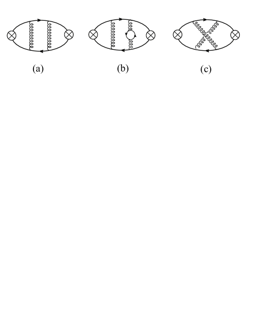
Figure 3: Different contributions to the pion correlator from Chen [84]

Quenched QCD is not a consistent theory, because omitting the fermion loops causes problems with unitarity. Bardeen [85] et al. have shown that there is a problem with the non-singlet $0^{++}$ correlator in quenched QCD. The problem can be understood using quenched chiral perturbation theory. The non-singlet $0^{++}$ propagator contains an intermediate state of $\eta^{\prime}-\pi$. The removal of fermion loops in quenched QCD has a big effect on the $\eta^{\prime}$ propagator. The result is that a ghost state contributes to the scalar correlator, that makes the expression in equation 23 inappropriate to extract masses from the calculation. Bardeen et al. [85] predict that the ghost state will make the $a_{0}$ mass increase as the quark mass is reduced below a certain point. This behaviour was observed by Weingarten and Lee [86] for small box sizes (L $\leq$ 1.6 fm). The negative scalar correlator was also seen by DeGrand [62] in a study of point to point correlators. Damgaard et al. [87] also discuss the scalar correlator in quenched QCD.

One major problem with quenched QCD is that it does not suppress zero eigenvalues of the fermion operator [88]. A quark propagator is the inverse of the fermion operator, so eigenvalues of the fermion operator that are zero, or close to zero, cause problems with the calculation of the quark propagator. In unquenched QCD, gauge configurations that produce zero eigenvalues in the fermion operator are suppressed by the determinant in the measure. Gauge configurations in quenched QCD that produce an eigenvalue spectrum that cause problems for the computation of the propagator are known as “exceptional configurations”. Zero modes of the fermion operator can be caused by topology structures in the gauge configuration. The problem with exceptional configurations get worse as the quark mass is reduced. The new class of actions, described in the appendix A that have better chiral symmetry properties, do not have problems with exceptional configurations

Please note that this section should not be taken as an apology for quenched QCD. As computers and algorithms get faster the parameters of unquenched lattice QCD are getting “closer” to their physical values. Hopefully quenched QCD calculations will fade away.

3.2 LATTICE SPACING ERRORS

Lattice QCD calculations produce results in units of the lattice spacing. One experimental number must be used to calculate the lattice spacing from:

$$a=am_{latt}^{X}/m_{expt}^{X}$$ (47)

As the lattice spacing goes to zero any choice of $m_{expt}^{X}$ should produce the same lattice spacing – this is known scaling. Unfortunately, no calculations are in this regime yet. The recent unquenched calculations by the MILC collaboration [89, 90, 91] may be close.

Popular choices to set the scale are the mass of the rho, mass splitting between the S and P wave mesons in charmonium, and a quantity defined from the lattice potential called $r_{0}$. The quantity $r_{0}$ [92, 93] is defined in terms of the static potential $V(r)$ measured on the lattice.

$$r_{0}^{2}\frac{dV}{dr}\mid_{r_{0}}=1.65$$ (48)

Many potential [92] models predict $r_{0}$ $\sim$ 0.5 fm. The value of $r_{0}$ can not be measured experimentally, but is “easy” to measure on the lattice. The value of $r_{0}$ is a modern generalisation of the string tension. Although it may seem a little strange to use $r_{0}$ to calculate the lattice spacing, when it is not directly known from experiment. There are problems with all methods to set the lattice spacing. For example, to set the scale from the mass of the rho meson requires a long extrapolation in light quark mass. Also it is not clear how to deal with the decay width of the rho meson in Euclidean space.

The physics results from lattice calculations should be independent of the lattice spacing. A new lattice spacing is obtained by running at a different value of the coupling in equation 7. In principle the dependence of quantities on the coupling can be determined from renormalisation group equations:

$$\beta(g_{0})=a\frac{d}{da}g_{0}(a)$$ (49)

The renormalisation group equations can be solved to give the dependence of the lattice spacing on the coupling [94].

$$a=\frac{1}{\Lambda}(g_{0}^{2}\gamma_{0})^{-\gamma_{1}/(2\gamma_{0}^{2})}e^{(-1/(2\gamma_{0}g_{0}^{2}))}(1+O(g_{0}^{2}))$$ (50)

The $e^{-1/(2\gamma_{0}g_{0}^{2})}$ term in equation 50 prevents any weak coupling expansion converging for masses.

Equation 50 is not often used in lattice QCD calculations. The bare coupling $g_{0}$ does not produce very convergent series. If quantities, such as Wilson loops are computed in perturbation theory and from numerical lattice calculations the agreement between the two methods is very poor. Typically couplings defined in terms of more “physical” quantities, such as the plaquette are used in lattice perturbative calculations [38].

Allton [95] tried to use variants of 50 with some of the improved couplings. He also tried to model the effect of the irrelevant operators. An example of Allton’s result for the lattice spacing determined from the $\rho$ mass as a function of the inverse coupling is in figure 4.

Figure 4: The lattice spacing determined from the mass of the rho meson as a function of the coupling ($\beta=\frac{6}{g^{2}}$) [95]

There are corrections to equation 50 from lattice spacing errors. For example the Wilson fermion action in equation 9 differs from the continuum Dirac action by errors that are $O(a)$. The lattice spacing corrections can be written in terms of operators in a Lagrangian. These operators are known as irrelevant. Ratios of dimensional quantities are extrapolated to the continuum limit using a simple polynomial.

$$\frac{am_{1}}{am_{2}}=\frac{am_{1}^{cont}}{am_{2}^{cont}}+xa+O(a^{2})$$ (51)

The improvement program discussed in appendix A designs fermion actions to reduce the lattice spacing dependence of ratios of dimensional quantities. When computationally feasible, calculations are done at (least) three lattice spacings and the results are extrapolated to the continuum. This was the strategy of the large scale GF11 [3] and CP-PACS calculations [96].

It is very important to know the exact functional form of the lattice spacing dependence of the lattice results for a reliable extrapolation to the continuum. The quantum field theory nature of the field renormalises the correction polynomial. There are potentially $O(a^{n}g^{m})$ errors. This is particularly a problem for states with a mass that is comparable to the inverse lattice spacing. There is physical argument that the Compton wavelength of a hadron should be greater than the lattice spacing. This is a problem for heavy quarks such as charm and bottom, that is usually solved by the use of effective field theories [10, 11, 21]. The masses of the excited light hadrons are large relative to the inverse lattice spacing, so there may be problems with the continuum extrapolations.

There have been a number of cases where problems with continuum extrapolations have been found. For example Morningstar and Peardon [97] found that the mass of the $0^{++}$ glueball had a very strange dependence on the lattice spacing. Morningstar and Peardon [98] had to modify the gauge action to obtain results that allowed a controlled continuum extrapolation. The ALPHA collaboration [99] discuss the problems of extrapolating the renormalisation constant associated with the operator corresponding to the average momentum of non-singlet parton densities to the continuum limit, when the exact lattice spacing dependence is not known.

In principle the formalism of lattice gauge theory does not put a restriction on the size of the lattice spacing used. The computational costs of lattice calculations are much lower at larger lattice spacings (see equation 46). However, there may be a minimum lattice spacing, set by the length scale of the important physics, under which the lattice calculations become unreliable [100].

There has been a lot of work to validate the instanton liquid model on the lattice [101]. Instantons are semi-classical objects in the gauge fields. The instanton liquid model models the gauge dynamics with a collection of instantons of different sizes. Some lattice studies claim to have determined that there is a peak in the distribution of the size of the instantons between 0.2 to 0.3 fm in quenched QCD [102, 103, 104]. If the above estimates are correct, then lattice spacings of at least 0.2 fm would be required to correctly include the dynamics of the instanton liquid on the lattice. However, determining the instanton content of a gauge configuration is non-trivial, so estimates of size distributions are controversial. At least one group claims to see evidence in gauge configurations against the instanton liquid model [105, 106].

There have been a few calculations of the hadron spectrum on lattices with lattice spacings as coarse as 0.4 fm [97, 107, 108, 109, 110]. There were no problems reported in these coarse lattice calculations, however only a few quantities were calculated.

Another complication for unquenched calculations is that the lattice spacing depends on the value of the sea quark mass [111]. as well as the coupling. This is shown in figure 5. The dependence of the lattice spacing on the sea quark mass is a complication, because for example the physical box size now depends on the quark mass.

Some groups prefer to tune the input parameters in their calculations so that the lattice spacing [89, 112] is fixed with varying sea quark mass. Other groups prefer to work with a fixed bare coupling [29].

Figure 5: Lattice spacing dependence on the sea quark mass $1/\kappa_{sea}$ from  [111].

3.3 QUARK MASS DEPENDENCE

The cost of lattice QCD calculations (see equation 46) forces the calculations to be done at unphysical large quark masses. The results of lattice calculations are extrapolated to physical quark masses using some functional form for the quark mass dependence. The dependence on the light quark masses is motivated from effective field theories such as chiral perturbation theory. The modern view is that the lattice QCD calculations do not need to be done at exactly the masses of the physical up and down quarks, but the results can be matched onto an effective theory [113]. In this section I briefly discuss the chiral extrapolation fit models used to extrapolate hadron masses from lattice QCD data to the physical points.

The relationship between effective theories and lattice QCD is symbiotic, because the results from lattice QCD calculations can also test effective field theory methods. The extrapolation of lattice QCD data with light quark masses is currently a “hot” and controversial topic in the lattice QCD community. The controversy is over the different ways to improve the convergence of the effective theory. There was a discussion panel on the different perspectives on using effective field theories to analyse lattice QCD data, at the lattice 2002 conference [114]. In section 5, I show that the masses of the quarks used in lattice calculations are getting lighter, that will help alleviate many problems.

In the past chiral perturbation theory provided functional forms that could used to analyse the quark mass dependence of lattice data. In practise, the extrapolations of lattice data were mostly done assuming a linear dependence on the quark mass [3], The mass dependence from effective field theory was essentially treated like a black box. However, a number of high profile studies [115] have shown that a deeper understanding of the physics behind the expressions from chiral perturbation theory is required. The subject of effective Lagrangians for hadronic physics is very large. The reviews by Georgi [116], Lepage [117] and Kaplan [118] contain introductions to the physical ideas behind effective field theory calculations. Scherer [119] reviews chiral perturbation theory for mesons and baryons.

The chiral perturbation theory for the lowest pseudoscalar particles is the perhaps the most “well defined” theory. The effective field theories for the vectors and baryon particles are perhaps more subtle with concerns about convergence of the expansion. In this section, I will briefly describe effective field theories, starting with the pseudoscalars and working up to nucleons via the vector particles. I will try to explain some of the physical pictures behind the functional dependence from effective field theories, rather than provide an exhaustive list of expressions to fit to.

In Georgi’s review [116] of the basic ideas behind effective theory, he quotes the essential principles behind effective field theory as

• A local Lagrangian is used.

• There are a finite numbers of parameters that describe the interaction each of dimension $(k-4)$.

• The coefficients of the interaction terms of dimension $(k-4)$ is less than or of the order of $(\frac{1}{M^{k}})$ where $E<M$ for some mass independent $k$.

The above principles allow that physical processes to be calculated to an accuracy of $(\frac{E}{M})^{k}$ for a process of energy $E$. The energy scale $M$ helps to organise the power counting. The accuracy of the results can be improved in a systematic way if more parameters are included. This is one of the main appeals of the formalism. As the energy of the process approaches $M$, then in the strict effective field theory paradigm, a new effective field theory should be used with new degrees of freedom [116]. For example, Fermi’s theory of weak interactions breaks down as the propagation of the $W$ becomes important. For these process the electroweak theory can be used.

The effective field theory idea can be applied to hadronic physics. Indeed historically, the origin of the effective field theory idea was in hadronic physics. A Lagrangian is written down in terms of hadron fields, as hadrons are the more appropriate degrees of freedom at low energies. The Lagrangian is chosen to have the same symmetries as QCD, hence in its domain of validity it should give the same physics results as QCD. This is known as Weinberg’s theorem [120].

For “large” momentum scales the quark and gluon degrees of freedom will become evident, so the theory based on the chiral Lagrangian with hadron fields must break down. Unfortunately, it is not clear what the next effective field theory is beyond the hadronic effective Lagrangian, because it is hard to compute anything in low energy QCD.

The lowest order chiral Lagrangian for pseudoscalars is

$${\cal L}_{2}=\frac{F^{2}}{4}\mbox{Tr}(\sum_{\mu}D_{\mu}V^{\dagger}D_{\mu}V-\chi^{\dagger}V-\chi V)$$ (52)

$$V(x)=e^{\phi(x)/F_{0}}$$ (53)

$$\phi(x)=\left(\begin{array}[]{ccc}\pi^{0}+\frac{1}{\sqrt{3}}\eta&\sqrt{2}\pi^{+}&\sqrt{2}K^{+}\\ \sqrt{2}\pi^{-}&-\pi^{0}+\frac{1}{\sqrt{3}}\eta&\sqrt{2}K^{0}\\ \sqrt{2}K^{-}&\sqrt{2}\overline{K}^{0}&-\frac{2}{\sqrt{3}}\eta\end{array}\right)$$ (54)

The expansion parameter [121] for the chiral Lagrangian of pseudoscalar mesons is

$$\lambda_{\chi}\sim m_{\rho}\sim 4\pi F_{\pi}\sim 1GeV$$ (55)

The power counting theorem of Weinberg [120] guarantees that the tree level Lagrangian in equation 52 will generate the $E^{4}$ Lagrangian and non-analytic functions.

The next order terms in the Lagrangian for the pseudoscalars are

$${\cal L}_{4}=\sum_{i=1}^{10}\alpha_{i}O_{i}$$ (56)

The coefficients $\alpha_{i}$ are independent of the pion mass. They represent the high momentum behaviour. The normalisation used in lattice calculations is connected to the one in Gasser and Leutwyler [122] by $\alpha_{i}=8(4\pi)^{2}L_{i}$. For example, one of the terms in the $O(p^{4})$ Lagrangian is

$$O_{1}=[\mbox{Tr}(D_{\mu}VD^{\mu}V^{\dagger})]^{2}$$ (57)

It can be convenient to have quarks with different masses in the sea, than those used in the valence correlators. In lattice QCD jargon, this is known as “partial quenching”. These partially quenched theories can provide information about the real unquenched world [123, 124, 125]. The chiral Lagrangian predicts [125, 126] the mass of the pion to depend on the sea and valence quark masses

$$M_{PS}^{2}=y_{12}(4\pi F_{0})^{2}[1 + \frac{1}{n_{f}}\left(\frac{y_{11}(y_{SS}-y_{11})\log y_{11}-y_{22}(y_{SS}-y_{22})\log y_{22}}{y_{22}-y_{11}}\right)$$ (58)

$$+ y_{12}(2\alpha_{8}-\alpha_{5})+y_{SS}N_{f}(2\alpha_{6}-\alpha_{4})]$$

The function $y_{ij}$ is related to the quark mass via

$$y_{ij}=\frac{B_{0}(m_{i}+m_{j})}{(4\pi F_{0})^{2}}$$ (59)

where $F_{0}$ is the pion decay constant. The leading order term in equation 58 represents the PCAC relation.

The terms like $\log y_{11}$ are known as “chiral logs” are caused by one loop diagrams. As the chiral logs are independent of the Gasser-Leutwyler coefficients ($\alpha_{4}$, $\alpha_{5}$, $\alpha_{6}$, $\alpha_{8}$), they are generic predictions of the chiral perturbation theory. A major goal of lattice QCD calculations is to detect the presence of the chiral logs. This will give confidence that the lattice QCD calculations are at masses where chiral perturbation theory is applicable (see [7] for a recent review of how close lattice calculations are to this goal).

There have been some attempts to use equation 58 to determine the Gasser-Leutwyler coefficients from lattice QCD [126, 127, 128, 129].

GL coeff	continuum	$n_{f}=2$ [130]
$\alpha_{5}(4\pi F_{\pi})$	$0.5\pm 0.6$	$1.22^{+11}_{-0.16}(stat)^{+23}_{-26}$
$\alpha_{8}(4\pi F_{\pi})$	$0.76\pm 0.4$	$0.79^{+5}_{-7}(stat)^{+21}_{-21}$

Table 1: where the mass of the sea quark is $m_{s}$ and the masses of the valence quarks are $m_{1}$ and $m_{2}$. Comparison of the results for the Gasser-Leutwyler coefficients from lattice QCD (with two flavors) [130], to non-lattice estimates [131]..

Table 1 contains some results for the Gasser-Leutwyler coefficients from a two flavour lattice QCD calculation at a fixed lattice spacing of around 0.1 fm [130], compared to some non-lattice estimates [131].

It is claimed that resonance exchange is largely responsible for the values for the values of the Gasser-Leutwyler coefficients [132, 131]. For example, in this approach the value of $\alpha_{5}$ is related to the properties of the scalar mesons.

$$\alpha_{5}^{scalar}=8(4\pi)^{2}\frac{c_{d}c_{m}}{M_{S}^{2}}$$ (60)

where $M_{S}$ is the mass of the non-singlet scalar and the parameters $c_{d}$ and $c_{m}$ are related to the decay of the scalar into two mesons.

The $\alpha_{5}$ and $\alpha_{8}$ coefficients are important to pin down the Kaplan-Manohar ambiguity [133] in the masses chiral Lagrangian at order O($p^{4}$). The latest results on estimating Gasser-Leutwyler coefficients using lattice QCD are reviewed by Wittig [7].

Most lattice QCD calculations do not calculate at light enough quarks so that the $log$ terms in equation 58 are apparent. In practise many groups extrapolate the squares of the light pseudoscalar meson as either linear or quadratic functions of the light quark masses. For example the CP-PACS collaboration [134] used fit models of the type

$$m_{PS}^{2}=b^{PS}_{S}m_{S}+b^{PS}_{V}m_{V}+c^{PS}_{S}m_{S}^{2}+c^{PS}_{V}m_{V}^{2}+c^{PS}_{SV}m_{V}m_{S}$$ (61)

for the mass of the pseudoscalar ($m^{PS}$) where $m_{S}$ is the mass of the sea quark and $m_{V}$ is the mass of a valence quark.

In traditional chiral perturbation theory (see [119] for a review) framework $B$ is

$$B_{0}=-\frac{1}{3F_{0}^{2}}\langle\overline{q}q\rangle$$ (62)

It is possible that $B_{0}$ is quite small [135, 136], say of the order of the pion decay constant. In this scenario the higher order terms in quark mass become important. There is a formalism called generalised chiral perturbation theory [136] that is general enough to work with a small $B_{0}$. The chiral condensate has been computed using quenched lattice QCD [137, 138]. The generalised chiral perturbation theory predictions have been compared to some lattice data by Ecker [139]. The next generation of experiments may be able to provide evidence for the standard picture of a large $B_{0}$.

Morozumi, Sanda, and Soni [140] used a linear sigma model to study lattice QCD data. Their motivation was that the quark masses on lattice QCD calculations may be too large for traditional chiral perturbation to be appropriate.

There is also a version of chiral perturbation theory developed for quenched QCD, by Morel [141], Sharpe [142], Bernard and Golterman [143]. Quenched QCD is considered as QCD with scalar ghost quarks. The determinant of the ghost quarks cancels the determinant of the quarks. The relevant symmetry for this theory is $U(3\mid 3)\times U(3\mid 3)$. This is a graded symmetry, because it mixes fermions and bosons. The chiral Lagrangian is written down in terms of a unitary field that transform under the graded symmetry group.

In this section, I follow the review by Golterman [144]. The problems with quenched QCD can be seen by looking at the Lagrangian for the $\eta^{\prime}$ and $\overline{\eta}^{\prime}$ (the ghost partner of the $\eta^{\prime}$).

$${\cal L}_{\eta^{\prime}} = \frac{1}{2}(\partial_{\mu}\eta^{\prime})^{2}-\frac{1}{2}(\partial_{\mu}\overline{\eta}^{\prime})^{2}+$$ (63)

$$\frac{1}{2}m_{\pi}^{2}((\eta^{\prime})^{2}-(\overline{\eta}^{\prime})^{2})+\frac{1}{2}\mu^{2}(\eta^{\prime}-\overline{\eta}^{\prime})^{2}+\frac{1}{2}\alpha^{2}(\partial_{\mu}(\eta^{\prime}-\overline{\eta}^{\prime}))^{2}$$

The propagator for the $\eta^{\prime}$ can be derived from equation 63.

$$S_{\eta^{\prime}}(p)=\frac{1}{p^{2}+m_{\pi}^{2}}-\frac{\mu^{2}+\alpha p^{2}}{(p^{2}+m_{\pi}^{2})^{2}}$$ (64)

The double pole in equation 64 stops the $\eta^{\prime}$ decoupling in quenched chiral perturbation theory as $\mu$ gets large. This has a dramatic effect on the dependence of the meson masses on the light quark mass. For example the dependence of the square of the pion mass on the light quark mass $m_{q}$ is

$$m_{\pi}^{2}=Am_{q}(1+\delta(\log(Bm_{q}))+Cm_{q})$$ (65)

where $\delta$ is defined by

$$\delta=\frac{\mu^{2}}{24\pi^{2}f_{\pi}^{2}}$$ (66)

and $A$, $B$, and $C$ are functions of the parameters in the Lagrangian. In standard chiral perturbation theory, the $\delta$ term in equation 65 is replaced by $\frac{m_{\pi}^{2}}{(4\pi f_{\pi}^{2})}$. As the quark mass is reduced, equation 65 predicts that the pion mass will diverge. Values of $\delta$ from 0.05 to 0.30 have been obtained [7] from lattice data. It has been suggested [7] that the wide range in $\delta$ might be caused by finite volume effects in some calculations.

The effective Lagrangians, encountered so far, assume that the hadron masses are in the continuum limit. In practise most lattice calculation use the quark mass dependence at a fixed lattice spacing. The CP-PACS collaboration [96] have compared doing a chiral extrapolation at finite lattice spacing and then extrapolating to the continuum, versus taking the continuum limit, and the doing the chiral extrapolation. In quenched QCD, the CP-PACS collaboration [96] found that the two methods only differed at the $1.5\sigma$ level.

It is very expensive to generate unquenched gauge configurations with very different lattice spacings, so it would be very useful to have a formalism that allowed chiral extrapolations at a fixed lattice spacing. Rupak and Shoresh [145] have developed a chiral perturbation theory formalism that includes $O(a)$ lattice spacing errors for the Wilson action. This type of formalism had already been used to study the phase of lattice QCD with Wilson fermions [146]. An additional parameter $\rho$ is introduced

$$\rho\equiv 2W_{0}ac_{SW}$$ (67)

where $W_{0}$ is an unknown parameter and $c_{SW}$ is defined in the appendix. This makes the expansion a double expansion in $\frac{p^{2}}{\Lambda_{\chi}^{2}}$ and $\frac{\rho}{\Lambda_{\chi}}$.

$${\cal L}_{2}=\frac{F^{2}}{4}\mbox{tr}(\sum_{\mu}D_{\mu}V^{\dagger}D_{\mu}V)-\frac{F^{2}}{4}\mbox{tr}((\chi+\rho)V+V(\chi^{\dagger}+\rho^{\dagger}))$$ (68)

The Lagrangian in equation 68 is starting to be used to analyse the results from lattice QCD calculations [147].

For vector mesons it less clear how to write down an appropriate Lagrangian than for the pseudoscalar mesons. There are a variety of different Lagrangians for vector mesons [148, 149, 150, 151], most of which are equivalent. A relativistic effective Lagrangian for the vector mesons [150] is

$${\cal L}=-\frac{1}{4}\mbox{Tr}(D_{\mu}V_{\nu}-D_{\nu}V_{\mu})^{2}+\frac{1}{2}M_{V}^{2}\mbox{Tr}(V_{\nu}V^{\nu})$$ (69)

where $V_{\nu}$ contains the vector mesons. As discussed earlier in this section, a crucial ingredient of the effective field theory formalism is that a power counting scheme can be set up. The large mass of the vector mesons complicates the power counting, hence other formalisms have been developed. Jenkins et al. [151] wrote down a heavy meson effective field theory for vector mesons.

In the heavy meson formalism the velocity $v$ with $v^{2}=1$ is introduced. Only the residual momentum ($p$) of vector mesons enters the effective theory.

$$k_{V}=M_{V}v+p$$ (70)

In the large $N_{c}$ limit the meson fields live inside $N_{\mu}$.

$$N_{\mu}=\left(\begin{array}[]{ccc}\rho^{0}_{\mu}+\frac{1}{\sqrt{2}}\omega_{\mu}&\rho^{+}_{\mu}&K^{\star+}_{\mu}\\ \rho^{-}_{\mu}&-\frac{1}{\sqrt{2}}\rho^{0}_{\mu}+\frac{1}{\sqrt{2}}\omega_{\mu}^{0}&K^{\star 0}_{\mu}\\ K^{\star-}&\overline{K}^{\star 0}_{\mu}&\phi_{\mu}\end{array}\right)$$ (71)

The Lagrangian for the heavy vector mesons (in the large $N_{c}$ and massless limit ) is

$${\cal L}=-i\mbox{Tr}N_{\mu}^{\dagger}(v.{\cal D})N^{\mu}-ig_{2}\mbox{Tr}\{N_{\mu}^{\dagger},N_{\nu}\}A_{\lambda}v_{\sigma}\epsilon^{\mu\nu\lambda\sigma}$$ (72)

The connection between the Lagrangian in equation 69 and the Lagrangian in equation 72 is discussed by the Bijnens et al. [150].

At one loop the correction to the $\rho$ mass [151] is

$$\Delta m_{\rho}=-\frac{1}{12\pi^{2}f^{2}}(g_{2}^{2}(\frac{2}{3}m_{\pi}^{3}+2m_{k}^{3}+\frac{2}{3}m_{\eta}^{3})+g_{1}^{2}(m_{\pi}^{3}))$$ (73)

where $g_{1}$ and $g_{2}$ are parameters (related to meson decay) in the heavy vector Lagrangian and $f$ is the pion decay constant. The next order in the expansion of the masses of vector mesons is in the paper by Bijnens et al. [150]. The equivalent expression in quenched and partially quenched chiral perturbation theory has been computed by Booth et al. [152] and Chow and Ray [153]. The heavy vector formalism suggests that for degenerate unquenched quarks the mass of the vector mass should depend on the quark mass $m_{q}$ like

$$M^{Vec}=M^{Vec}_{0}+M^{Vec}_{1}m_{q}+M^{Vec}_{2}m_{q}^{3/2}+O(m_{q}^{2})$$ (74)

In practise it has been found to be difficult to detect the presence of the $m_{q}^{3/2}$ term in equation 74 from recent lattice calculations. The mass of the light vector particle from lattice QCD calculations is usually extrapolated to the physical point using a function that is linear or quadratic in the quark mass. For example the CP-PACS collaboration [134] used the fit model

$$M^{Vec}=A^{Vec}+B_{S}^{Vec}m_{S}+B_{V}^{Vec}m_{V}+C_{S}^{Vec}m_{S}^{2}+C_{V}^{Vec}m_{V}^{2}+C_{V}^{Vec}m_{V}m_{S}$$ (75)

to extrapolate the mass of the vector meson ($M_{vec}$) in terms of the sea ($m_{S}$) and valence ($m_{V}$) quark masses in their unquenched calculations. CP-PACS [134] also investigated the inclusion of terms from the one loop calculation of the correction to the rho mass in equation 73.

There is an added complication for the functional dependence of the mass of the $\rho$ meson on the light quark mass, because in principle the rho can decay into two pions (see section 10) . This decay threshold complicates the chiral extrapolation model. The first person to do an analysis of this problem for the $\rho$ meson in lattice QCD was DeGrand [154]. There was further work done by Leinbweber amd Cohen [155]. The effect of decay thresholds on hadron masses is also a problem for the quark model [156, 235].

The Adelaide group [157] have studied the issue of the effect of the rho decay on the chiral extrapolation model of the rho meson mass in more detail. The physical motivation behind Adelaide group’s program in the extrapolation of hadron masses in the light quark mass has been reviewed by Thomas [158].

The mass of the rho is shifted by $\pi-\pi$ and $\pi-\omega$ intermediate states. The effect of the two meson intermediates states can be found by computing the Feynman diagrams in figure 6 from an effective field Lagrangian. The self energies from the $\pi-\pi$ ($\Sigma^{\rho}_{\pi\pi}$) and the $\pi-\omega$ ($\Sigma^{\rho}_{\pi\omega}$) intermediate states. renormalize the mass of the $\rho$ meson.

$$m_{\rho}=\sqrt{m_{0}^{2}+\Sigma^{\rho}_{\pi\pi}+\Sigma^{\rho}_{\pi\omega}}$$ (76)

Figure 6: Self energy contributions to the mass of the rho meson.

To explain the idea, I will consider the self energy corrections from $\pi-\omega$ intermediate states in more detail.

$$\Sigma^{\rho}_{\pi\omega}=-\frac{g_{\omega\rho\pi}^{2}\mu_{\rho}}{12\pi^{2}}\int_{0}^{\infty}\frac{dkk^{4}u^{2}_{\omega\pi}(k)}{w_{\pi}(k)^{2}}$$ (77)

where

$$w_{\pi}(k)^{2}=k^{2}+m_{\pi}^{2}$$ (78)

and $\mu_{\rho}$ is the physical mass of the $\rho$ meson. The integral for the $\Sigma^{\rho}_{\pi\pi}$ is similar, but the algebra is more complicated.

As the momentum increases the effective field theory description of the physics in terms of meson field breaks down. Adelaide prefer to parameterise the breakdown of the effective field theory by introducing a form factor $u_{\omega\pi}(k)$ at the interaction between the two pseudoscalars mesons and the vector meson. A dipole form factor is used in equation 77.

$$u_{\omega\pi}(k)=(\frac{\Lambda_{\pi\omega}^{2}-\mu_{\pi}^{2}}{\Lambda_{\pi\omega}^{2}+k^{2}})^{2}$$ (79)

The $\Lambda_{\pi\omega}$ parameter is a (energy) scale associated with the finite extent of the hadrons. This is a fit parameter that the Adelaide group [157] determine from lattice data. They obtain [157] $\Lambda_{\pi\omega}$ = 630 MeV.

It is instructive to look at the self energy $\Sigma^{\rho}_{\pi\omega}$ with a sharp cut off

$$\Sigma^{\rho}_{\pi\omega}=-\frac{g_{\omega\rho\pi}\mu_{\rho}}{12\pi^{2}}(m_{\pi}^{3}\arctan(\frac{\Lambda}{m_{\pi}})+\Lambda^{3}-\Lambda m_{\pi}^{2})$$ (80)

There is strong dependence on $\Lambda$ in equation 80. The $\Sigma^{\rho}_{\pi\omega}$ term contains the $m_{\pi}^{3}$ term of chiral perturbation theory.

In the Adelaide approach [157] the fit model used to extrapolate the mass of the rho meson in terms of the quark mass is in equation 81.

$$m_{\rho}=c_{0}+c_{1}m_{\pi}^{2}+\frac{\Sigma^{\rho}_{\pi\omega}(\Lambda_{\pi\omega},m_{\pi})+\Sigma^{\rho}_{\pi\pi}(\Lambda_{\pi\pi},m_{\pi})}{2(c_{0}+c_{1}m_{\pi}^{2})}$$ (81)

This is a replacement for the chiral extrapolation model in equation 74.

The Adelaide group [157] note that the coefficient of the $m_{\pi}^{3}$ term in equation 73 is known, hence this is a constraint on the fits from the lattice data. However, the actual fits to the mass of the rho particle from lattice QCD, do not reproduce the known coefficient in equation 73. When the Adelaide group [157] fit the expression in equation 81 to the mass of the rho at the coarse lattice spacings from calculations by UKQCD [111] and CP-PACS, the correct coefficient is obtained.

It is interesting to compare the Adelaide group’s [157] approach to the chiral extrapolation of the mass of the rho meson to a more “traditional” effective field theory calculation. Equation 77 looks similar to a perturbative calculation with a cut off. In an effective field theory calculation terms with powers of $\Lambda$ would be absorbed into the counter terms. In a field theory with a cut off, the actual cut off should have no effect on the dynamics in the effective theory. A strong dependence on the cut off would signify the breakdown of the effective theory. The lecture notes by Lepage discuss the connection between a cut off field theory and renormalisation in nuclear physics [117].

In his review on effective field theories Georgi [116] quotes Sidney Coleman as asking “what’s wrong with form factors?” Georgi’s answer is “nothing”. My translation of Georgi’s more detailed answer to Coleman’s question is in the next paragraph.

Both the Adelaide group’s approach and effective field theory agree for low momentum scales, hence both formalisms can reproduce the non-analytic correction in equation 73 to the mass of the rho, however the two formalisms differ in the treatment of the large momentum behaviour. In the effective field theory paradigm the large momentum behaviour is parameterised by a local Lagrangian with terms that are ordered with a power counting scheme. In the Adelaide group’s approach the long distance physics is parameterised (presumably with Coleman’s blessing) by a form factor. In an ideal world, the use of an effective field theory is clearly superior to the use of a form factors as the accuracy of the approximation is controlled. For the rho and nucleon it is not obvious how to set up a power counting scheme in the energy (although people are trying). Also an effective field theory based on hadrons will no longer describe the physics at large momentum when the quark and gluon degrees of freedom become important, hence the use of a form factor may be a more pragmatic way to control the long distance behaviour of hadronic graphs. It may be easier to introduce decay thresholds in a form factor based approach. The hard part of a form factor based approach is controlling the errors from the approximate nature of the form factor. The Adelaide group [159] do check the sensitivity of their final results by using different form factors. For the light pseudoscalars, the standard effective field theory formalism is clearly superior.

There is a “tradition” of not using “strict” effective field theory techniques for the $\rho$ meson. For example DeGrand [154] used a twice subtracted dispersion relation to regulate the graph in figure 6.

Nucleons have also been incorporated into the Chiral Lagrangian approach (see [119] for a review).

$$\Psi=\left(\begin{array}[]{c}p\\ n\end{array}\right)$$ (82)

$${\cal L}_{\pi N}=\overline{\Psi}iD/-\hat{m_{N}}+\frac{\hat{g_{A}}}{2}\gamma_{\mu}\gamma_{5}u_{\mu}\Psi$$ (83)

where $\hat{m_{N}}$ and $\hat{g_{A}}$ are parameters in the chiral limit.

$$u^{2} = U$$ (84)

$$u_{\mu} = iu^{\dagger}\partial_{\mu}Uu^{\dagger}$$ (85)

$$\Gamma_{\mu} = \frac{1}{2}[u^{\dagger},\partial_{\mu}u]$$ (86)

$$D_{\mu} = \partial_{\mu}+\Gamma_{\mu}$$ (87)

$U$ is the $SU(2)$ matrix containing the pion fields.

There are a number of complications with baryon chiral perturbation based on the relativistic action over meson perturbation theory. As discussed earlier the power counting is the key principle in effective theory as it allows an estimate of the errors from the neglected terms. However, the nucleon mass in baryon chiral perturbation theory is the same order as $4\pi F_{0}$. This complicates the power counting. Also the expansion is linear in the small momentum.

Most modern baryon chiral perturbation theory calculations are done using ideas motivated from heavy quark effective field theory [160, 161]. The four momentum is factored into a velocity dependent part and a small residual momentum part.

$$p_{\mu}=mv_{\mu}+k_{\mu}$$ (88)

The baryon field is split into “large” and “small” fields.

$${\cal N}_{v} \equiv e^{imv.x}P_{v+}\Psi$$ (89)

$${\cal H}_{v} \equiv e^{imv.x}P_{v-}\Psi$$ (90)

where the projection operator is defined by

$$P_{v+/-}=\frac{1+v_{\nu}\gamma^{\nu}}{2}$$ (92)

The leading order Lagrangian for heavy baryon chiral perturbation theory (HBChPT) is

$${\cal L}_{\pi N}=\overline{{\cal N}}_{v}(iv.D+\frac{g_{A}}{2}S_{v}.u){\cal N}$$ (93)

where

$$S_{v}^{\mu}=\frac{i}{2}\gamma_{5}\sigma^{\mu\nu}v_{\nu}$$ (94)

In principle there are $\frac{1}{M_{Q}}$ corrections to equation 93. See the review article by [119] for a detailed comparison of the relativistic and heavy Lagrangians.

The final extrapolation formula for the nucleon mass $M_{N}$ as a function of the quark mass $m_{q}$ is:

$$M^{N}=M^{N}_{0}+m_{q}B+m_{q}^{3/2}C+....$$ (95)

The coefficient $C$ is negative and is a prediction of the formalism.

The convergence of baryonic chiral perturbation theory is very poor even in the continuum. On the lattice the pion masses are even larger, hence there are additional concerns about the convergence of the predictions. Using chiral perturbation theory, Borasoy and Meissner [162] computed the nucleon mass (and other quantities) using heavy baryonic chiral perturbation theory, including all quark mass terms up to and including the quadratic order. The result for the nucleon mass is in equation 96 for each order of the quark mass

$$M^{N}=\hat{m}(1+0.34-0.35+0.24)$$ (96)

where $\hat{m}$ = 767 MeV. Note this is not a lattice calculation. Although, when all the terms are summed up, the correction is small to the nucleon mass, there are clearly problems with the convergence of the series. The corrections to the masses of the $\Lambda$, $\Sigma$ and $\Xi$ baryons were also sizable.

Donoghue et al. [163] blame the poor convergence of baryoninc chiral perturbation theory on the use of dimensional regularisation. Donoghue et al. [163] argue that the distances below the size of the baryon in the effective field theory description breaks down, however the dimensionally regulated graphs include all length scales. The incorrect physics from the graphs is compensated by the counter terms in the Lagrangian. Unfortunately, this “compensation” makes the expansion poorly convergent. Lepage [117] also gives an example (from [164]) from nuclear physics where using a cut off gives a better representation of the physics than using minimal subtraction with dimensional regularisation.

The graph in equation 97 occurs at one loop for the baryon masses.

$$\int\frac{d^{4}k}{(2\pi)^{4}}\frac{k_{i}k_{j}}{(k_{0}-i\epsilon)(k^{2}-m^{2}+i\epsilon)}=-i\delta_{ij}\frac{I(m)}{24\pi}$$ (97)

In dimensional regularisation [165]

$$I_{dim-reg}(m)=m^{3}$$ (98)

The graph in equation 97 contributes the lowest non-analytic term in the octet masses ($M_{N}\propto m_{\pi}^{3}$). Donoghue et al. [163] point out that it is a bit suspicious that the result in equation 98 is finite when the integral in equation 97 is cubicly divergent.

Consider now equation 97 regulated with a dipole regulator.

$$\int\frac{d^{4}k}{(2\pi)^{4}}\frac{k_{i}k_{j}}{(k_{0}-i\epsilon)(k^{2}-m^{2}+i\epsilon)}(\frac{\Lambda^{2}}{\Lambda^{2}-k^{2}})=-i\delta_{ij}\frac{I_{\Lambda}(m)}{24\pi}$$ (99)

$$I_{\Lambda}(m)=\frac{1}{2}\Lambda^{4}\frac{2m+\Lambda}{m+\Lambda}^{2}$$ (100)

In the limit $m<\Lambda$ limit

$$I_{\Lambda}(m)\longrightarrow\frac{1}{2}\Lambda^{3}-\frac{1}{2}\Lambda m^{2}+m^{3}+...$$ (101)

Hence for small $m$ the result from dimensional regularisation is reproduced.

Up to this point the treatment of the integrals looks very similar to the approach originally advocated by the Adelaide group [159, 166]. However, Donoghue at al. [163] treat $\Lambda$ as a cut off. Strong dependence on $\Lambda$ is removed via renormalisation.

$$M_{0}^{r}=M_{0}-d\Lambda^{3}$$ (102)

where $d$ is a function of the other renormalised parameters in the Lagrangian (such as the pion decay constant). In the original work by the Adelaide group [159, 166]. the parameter $\Lambda$ was a physical number that could be extracted from the lattice data. In the formalism of Donoghue at al. [163], the physical results should not depend on $\Lambda$, although a weak dependence on $\Lambda$ may remain because the calculations are only done to one loop. The results for the mass of the nucleon as a function of the order of the expansion are

$$M^{N}=1.143-0.237+0.034=0.940\mbox{GeV}$$ (103)

with the cut off $\Lambda=400$ MeV. See [167] for a brief critique of formalism of Donoghue at al. [163].

The Adelaide group [159, 166] consider the one loop pion self energy to the nucleon and delta propagators. The method is essentially the same as the one applied to the chiral extrapolation of the rho mass. The Adelaide group [159, 166] fit model for the nucleon mass is

$$M_{N}=\alpha_{N}+\beta_{N}m_{\pi}^{2}+\sigma_{NN}(m_{\pi},\Lambda)+\sigma_{N\Delta}(m_{\pi},\Lambda)$$ (104)

where $\sigma$ come from one loop graphs. Equation 104 is a three parameter fit model: $\alpha$, $\beta$, and $\Lambda$.

The Adelaide group have applied the formalism of Donoghue at al. [163] to the analysis of lattice QCD data [168, 168] from CP-PACS. They have compared it with their previous formalism [168, 168].

Lewis and collaborators have studied the lattice regularisation of chiral perturbation theory [169, 170]. This type of calculation can not be used to quantify the lattice spacing dependence of lattice results [170], as the lattice spacing dependence of the two theories could very different. However, it is interesting to explore different regularisation schemes. There is renewed interest in the relativistic baryon Lagrangian, because a method [171]. called “infrared regularisation” allows a power counting scheme to be introduced (see [119] for a review).

All the above analysis of effective Lagrangians relied on perturbation theory to study the theory. Hoch and Horgan [172] used a numerical lattice calculation to study the $SU(2)\times SU(2)$ non-linear model, for pions and the nucleon. The unitary matrix $V$

$$V=\frac{1}{F}(\sigma.1+i\pi_{a}\tau_{a}\gamma_{5})$$ (105)

$$\sigma^{2}+\pi^{2}=F^{2}$$ (106)

$$S(V) = -\frac{1}{4}F^{2}\sum_{x}\mbox{tr}(\sum_{j=1}^{4}V(x)V(x+\mu_{j})^{\dagger}+V(x+\mu_{j})V^{\dagger}(x))$$

$$-\frac{1}{4}Fm_{0}^{2}\sum_{x}\mbox{tr}(U(x)+U(x)^{\dagger})$$

The numerical calculation was done with a small volume $8^{4}$, and no finite size study was done. The comparison of the lattice results with the perturbative results is complicated by the effect of the unknown parameters in the next order Lagrangian (equation  56 for example). Hoch and Horgan [172] found that the lattice calculation disagreed with the predictions of one loop perturbation theory for log divergent quantities.

A more conservative (some might say cowardly) approach to chiral extrapolations is to only interpolate the appropriate hadron masses to the mass of the strange quark, in an attempt to try to minimise the dependence of any results on uncontrolled extrapolation to the light quark masses. One formalism [173] for doing this is called the “method of planes”. Similar methods have been used by other groups (see for example [174, 175]). Obviously, this type of technique is not useful to get the nucleon mass. In unquenched QCD, the sea quark masses should be extrapolated to their physical values, so there is no way to avoid a chiral extrapolation even for heavy hadrons.

It is traditional to plot the hadron masses before any chiral extrapolations have been done, so as not to contaminate the raw lattice data from the computer with any theory. In an“Edinburgh plot” the ratio of the nucleon to rho mass is plotted against the pion to rho mass [176]. If there were no systematic errors, such as lattice spacing dependence, then the data should fall on a universal curve. It is also common to use $1/r_{0}$ [92] (see section 3.2) as a replacement for the mass of the $\rho$. There is also an APE plot that plots the ratio of the nucleon to rho mass against the square of the pion to rho mass [177]. This parameterisation is meant to have a smoother mass dependence than the Edinburgh plot.

3.4 FINITE SIZE EFFECTS.

The physical size of the lattice represents an obvious and an important systematic error. One simple way to estimate the size of a hadron is to consider its charge radius. For example, the proton’s charge radius is quoted as 0.870 (8) fm in the particle data table [6]. The sizes of all recent unquenched lattice QCD calculations are all above 1.6 fm (see section 5). The fact that all the physical lattice sizes were much bigger than the charge radius does not rule out finite size effects. In this section I will discuss some of the mechanisms thought to be behind finite size effects in lattice data.

A nice physical explanation of the origin of finite size effects for hadron masses has been presented by Fukugita et al. [178]. Consider a hadron in a box with length $L$ and periodic boundary conditions. Most lattice QCD calculations use periodic boundary conditions in space. The path integral formalism requires that the boundary conditions in time are anti-periodic [179], although many groups use periodic boundary condition in time as well as space. The finite size of the box will mean that a hadron will interact with periodic images a distance $L$ away. The origin of finite size effects is closely related to nuclear forces. The MILC collaboration have described a qualitative model for finite size effects based on nuclear density [83]. The nucleon is considered as part of nucleus comprising of the periodic images of the nucleon.

The self energy of the hadron ($\delta E$) will be

$$\delta E=\sum_{\underline{n}}V(\underline{n}L)$$ (108)

where $V(x)$ is the potential between two hadrons a distance $x$ apart. Various approximations to $V(x)$ give different functional forms for the dependence of the hadron mass on the volume.

In the large $L$ limit the potential is approximated by one particle exchange ($e^{-mr}/r$). The interaction energy goes like $V(0)+6V(L)$, so the dependence of the hadron mass will be $\sim e^{-m_{\pi}L}$. This argument can be made rigorous [180, 181].

It is useful to consider equation 108 in momentum space using the Poisson resummation formulae.

$$\delta E=\frac{1}{L^{3}}\sum_{\underline{n}}\hat{V}(\underline{n}\frac{2\pi}{L})$$ (109)

A more general expression for the potential between two hadrons can be derived if the spatial size of the hadron is modelled with a form factor $F(k)$.

$$\hat{V}(k)=\frac{F(k)^{2}}{k^{2}+m^{2}}$$ (110)

Momentum is quantised on the lattice in quanta of $\frac{2\pi a}{L}$. In physical units the value of a quantum of momentum is around 1 GeV, hence the $\underline{k}=\underline{0}$ term in equation 109 should dominate the sum. Therefore this model predicts that the masses should depend on the box size like:

$$M=M_{\infty}+cL^{-3}$$ (111)

This model is physically plausible but not a rigorous consequence of QCD. Fukugita et al. [178] noted their data could also be fit to the functional form.

$$m^{2}=m_{\infty}^{2}+c\frac{1}{L^{3}}$$ (112)

rather then equation 111. Unfortunately only the theory for the regime of point particle interacting at large distances is really rigorous [180, 181]..

Chiral perturbation theory can be used to compute finite volume corrections. For example the ALPHA/UKQCD collaboration have used [182] a chiral perturbation theory calculation by  [183] Gasser and Leutwyler to estimate the dependence of the pion mass $m_{PS}(L)$ on the box size $L$.

$$\frac{m_{PS}(L)}{m_{PS}(\infty)}=1+\frac{1}{N_{f}}\frac{m_{PS}^{2}}{F_{PS}^{2}}g(m_{PS}L)$$ (113)

$$g(z)=\frac{1}{8\pi^{2}z^{2}}\int_{0}^{\infty}\frac{dx}{x^{2}}e^{-z^{2}x-1/(4x)}$$ (114)

Garden et al. [182] used equations 113 and 114 to show that the error in $m_{PS}$ was 0.1 % for $m_{PS}L>4.3$. This an example of the rule thumb that finite size effects in hadron masses become a concern for $m_{PS}L<4$. Colangelo et al. [184] are extending equation 113 to the next order. Ali Khan et al. [185] have started to use chiral perturbation theory to study the finite size effects on the nucleon.

It would be useful if some insight could be gained from finite size effects in quenched QCD that could be applied to unquenched QCD where the volumes are smaller. Unfortunately, there are theoretical arguments [186] that show that finite size effects in the unquenched QCD will be larger than in the quenched QCD. A propagator for a meson can be formally be written in terms of gauge invariant paths. Conceptually this can be understood using the hopping parameter expansion. The quark propagators are expanded in terms of the $\kappa$ parameter. The hopping parameter expansion [187] was used in early numerical lattice QCD calculations, but was found not to be very convergent for light quarks.

$$c(t)=\sum_{C}\kappa_{val}^{L(C)}\langle W(C)\rangle+\sum_{C^{\prime}}\kappa_{val}^{L(C^{\prime})}\sigma_{val}\langle P(C^{\prime})\rangle$$ (115)

where $W(C)$ are closed Wilson loops inside the lattice of length $L(C)$. $P(C^{\prime})$ are Polykov lines that wrap around the lattice in the space direction. The $\sigma_{val}$ parameter is 1 for periodic boundary conditions and $-1$ for anti-periodic boundary conditions for Polykov lines that wrap around the lattice an odd number of times.

In quenched QCD $\langle P(C^{\prime})\rangle=0$ because of a $Z_{3}$ symmetry of the pure gauge action, so only the first term in equation 115 contributes to the correlator $c(t)$. The centre of SU(3), the elements that commute with all the elements of SU(3), is the $Z(3)$ group [17]. The Wilson gauge action is invariant under the gauge links being multiplied by a member of the centre of the group on each time plane. In unquenched QCD, the $Z_{3}$ symmetry is broken by the quark action, so both Wilson loop and Polyakov lines contribute to the correlators. There is no clear connection between the arguments based on equation 115 and the nuclear force and chiral perturbation formalism for finite size effects.

In their large scale quenched QCD spectroscopy calculations the CP-PACS collaboration kept the box to be 3 fm [96], so did not apply any corrections for the finite size of the lattice. Using the finite size estimate from previous calculations CP-PACS [96] estimated that the finite size effects were of the order 0.6 %. The GF11 group [4] did a finite size study at a coarse lattice spacing ($a$ = 0.17 fm). The results for ratios of hadron masses at finer lattice spacings were then extrapolated to the infinite volume limit using the estimated mass shift at the coarse lattice spacing. Gottlieb [27] gives a detailed critique of the method used by the GF11 group to extrapolate their mass ratios to the infinite volume.

If a formalism could be developed that would predict the dependence of hadron masses on the box size, then this would help make the calculations cheaper (see equation 46). The additional savings in computer time could be spent on reducing the size of the light quark masses used in the calculations [188]. Gottlieb [27] suggested, the only way to control finite size effects is to keep increasing the box size until the masses no longer change.

The finite box size is not always a bad thing. The size of the box has been used to advantage in lattice QCD calculations (see [189] for a review). A definition of the coupling is chosen that is proportional to $1/L$ (where $L$ is the length of one side of the lattice). A recursive scheme is setup that studies the change in coupling as the length of the lattice side $L$ is halved. The Femtouniverse, introduced by Bjorken [190], is a useful regime to study QCD in. There is a chiral perturbative expansion based on the limit $m_{\pi}<<\frac{1}{L}$ (see [87] for a modern application). See Van Baal [191] for a discussion of the usefulness of the finite volume on QCD.

It seems possible to run calculations in a big enough box to do realistic calculations. So the prospects are good for a first principles lattice calculation of hadron masses without resort to approximations in simulations of that kind required in condensed matter systems in simulations of macroscopic size systems.

4 AN ANALYSIS Of SOME LATTICE DATA

To consolidate the previous material, I will work over a simple analysis of some lattice QCD data. I think it is helpful to understand the steps in lattice QCD calculation, if the ideal case where QCD could be solved analytically is considered first. All the masses of the hadrons would be known as a function of the parameters of QCD: quark masses ($m_{i}$) and coupling $g$.

$$M_{H}=f_{H}(m_{u},m_{d},m_{s},m_{c},m_{b},g)$$ (116)

As the masses and coupling are not determined by QCD, the equation for all the hadrons $H$ would have to be solved to get the parameters. The solution would be checked for consistency that a single set of parameters could reproduce the entire hadron spectrum. For a calculation of a form factor, the master function $f_{H}$ would also depend on the momentum.

The formalism of lattice QCD is in some sense is a discrete approximation to the function $f_{H}$. The result from calculation would be a table of numbers:

$$M_{H}=f_{H}^{latt}(m_{u},m_{d},m_{s},m_{c},m_{b},g,L,a)$$ (117)

An individual lattice calculation would also depend on the lattice spacing and lattice volume. Lattice calculations have to be done at a number of different lattice spacings and volumes to extrapolate the dependence of $f_{H}^{latt}$ on $L$ and $a$.

By doing calculations with a number of different parameters the results can be combined to produce physical results in much the same way that could be done if the exact solution was known. In particular the lattice spacing and lattice volume have be extrapolated away to get access to the function $f_{H}$.

To understand the procedure in more detail, I will work through a naive analysis of some lattice QCD data from the UKQCD collaboration [192]. Table 2 contains the results for the mass of the $\pi$ and $\rho$ particles in lattice units from a quenched QCD [192]. The lattice volume was $24^{3}\;48$, $\beta$ = 6.2, and the ensemble size was 216. The clover action using the ALPHA coefficients was used. To use the data in table 2, the secret language of the lattice QCD cabal must be converted to the working jargon of the continuum physicist.

The ensemble size of 216 means that 216 snapshots of the vacuum (the value of $N$ in equation 18) were used to compute estimates of the $\rho$ and $\pi$ correlators. A supercomputer was used to compute the correlators for each gauge configuration from quark propagators (see equation 18). The masses were calculated by fitting the correlator to a fit model of the form in equation 23, using a $\chi^{2}$ minimiser such as MINUIT [193]. The error bars in the table in equation 2 come from a statistical procedure called the “bootstrap” method [194].

$\kappa$	$am_{\pi}$	$am_{\rho}$
0.13460	$0.2803^{+15}_{-10}$	$0.3887^{+32}_{-28}$
0.13510	$0.2149^{+19}_{-14}$	$0.3531^{+55}_{-51}$
0.13530	$0.1836^{+23}_{-18}$	$0.3414^{+72}_{-82}$

Table 2: Lattice QCD data for the masses of the pion and rho from lattice QCD calculations from UKQCD [192]

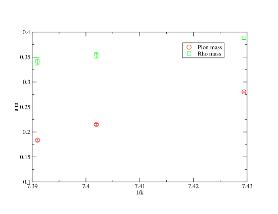
Figure 7: Rho and pion masses in lattice units as a function of inverse kappa value. The data set had $\beta=6.2,andavolumeof24^{3}48$. The fermion operator was the non-perturbatively improved clover operator.

A table of numbers of hadron masses (or even a graph) is not too useful. A better way to encapsulate the hadron masses as a function of quark mass is to use them to tune effective Lagrangians, as discussed in section 3.3. To plot the data in table 2 in a more physical form, I convert from the $\kappa$ value to the quark mass

$$m_{q}=\frac{1}{2}(\frac{1}{\kappa}-\frac{1}{\kappa_{crit}})$$ (118)

There are additional $O(a)$ corrections to equation 118 [189]. The $\kappa_{crit}$ parameter is required because clover fermions break chiral symmetry. The value of $\kappa_{crit}$ is the chosen to give a zero pion mass. Equation 118 is the basis of the computation of the masses of quarks from lattice QCD. However, perturbative factors are required to convert the quark mass to a standard scheme and scale. This perturbative “matching” can be involved, so the value of the quark mass is rarely used to indicate how light a lattice calculation is.

The simplest thing to do is to use a fit model in equation 119.

$$m_{PS}^{2}=S_{PS}m_{q}$$ (119)

There are classes of fermion actions (see appendix A), such as staggered or Ginsparg-Wilson actions, that do not have an additive renormalisation.

A simple fit to the data in table 2 with the fit model in equations 119 and 118 gives $\kappa_{crit}=0.135828(6)$, to be compared to $\kappa_{crit}=0.135818^{+18}_{-17}$ from the explicit analysis from UKQCD that included a $O(a)$ correction term.

To simplify the analysis, I will assume that the physical mass of the light quark is zero. I fit the data for the mass of the rho in table 2 to the model in equation 120.

$$m_{V}=A_{V}+S_{V}m_{q}$$ (120)

The result for the $A_{V}$ parameter is $0.304(2)$. If the mass of the light quark is assumed to be zero, then $am_{\rho}=0.304$, hence the lattice spacing is 2530 MeV (using $m_{\rho}=770$ MeV). This can be compared against the $a^{-1}$ = 2963 MeV from $r_{0}$ [195].

As the masses of quarks get lighter more sophisticated fit models based on the ideas in section 3.3 can be used. Although the basic ideas behind the analysis outlined in this section are correct, there are many improvements that can be made, particularly if the rho and pion correlators for each configuration are available.

5 PARAMETER VALUES OF LATTICE QCD CALCULATIONS

The results from unquenched lattice QCD calculations, with the lattice spacing and finite size effects accounted for, are the results from QCD at the physical parameters of the calculation. Hence a key issue in unquenched calculations is how close the parameters are to the physical parameters. For example, as discussed in section 3.3, ideally the masses of the quarks must be light enough to match the lattice results to chiral perturbation theory. The parameters used in a lattice calculation are usually dictated by the amount of computer time available, or what gauge configurations are publicly available.

In this section, I will describe the current state of the art in the parameters used in lattice QCD calculations of the hadron spectrum. It is not entirely obvious which parameters to use to characterise a lattice calculation. The obvious choice of using quark masses is complicated by the need for renormalisation and running. To show how light the quarks are in a calculation, I plot the ratio of the pseudoscalar mass to the vector mass for as a function of lattice spacing. The danger of this type of plot is that it says nothing about finite size effects. I usually just show the ratio for the lightest quark mass, as this is the most computationally most expensive point. The error bars on the ratio gives some indication on the statistical sample size. I have always used a lattice spacing defined by $r_{0}=0.49fm$ (see section 3.2).

In figure 8, I plot the smallest pseudoscalar mass to vector mass ratio as a function of lattice spacing for some recent large quenched calculations from the following collaborations: GF11 [3, 4], CP-PACS [196], UKQCD [192] BGR [197], and ALPHA [198].

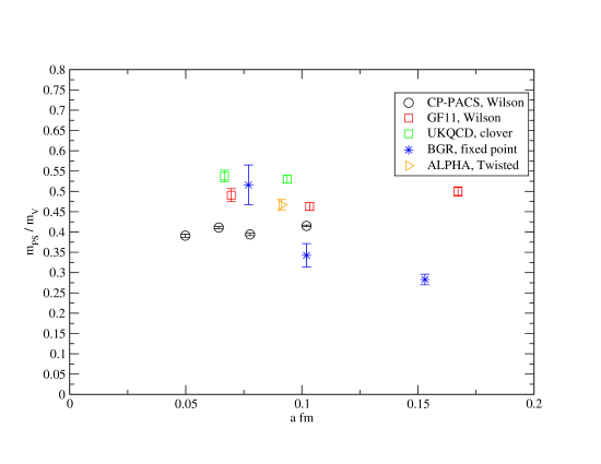
Figure 8: Smallest ratio of pseudoscalar mass to vector mass as a function of lattice spacing for a number of quenched QCD calculations. The labels have the collaboration name followed by the type of fermion operator.

The improvements in parameters between the GF11 calculation [3, 4], at the start of 1990’s and the CP-PACS calculation [196] at the end of 1990’s can clearly be seen in the figure.

Both the main benchmark calculations by CP-PACS [196] and GF11 [3, 4] used both the Wilson fermion and gauge actions. As I discuss in section A, lattice QCD actions with better properties have been developed. For example, the point in figure 8 from UKQCD used the clover fermion action. The clover action is designed to have smaller lattice spacing errors compared to the Wilson action. Unfortunately, the calculations by UKQCD [192] and QCDSF [199] that used the non-perturbative improved clover action reported problems with exceptional configurations, hence for those lattice spacings the light quark masses can not be reduced further at these lattice spacings. There is a formalism called twisted mass QCD [198] that is a natural extension of the clover action, that can be used to explore the light quark mass regime [200].

To reach lighter quark masses, it seems likely, that new fermion actions such as the overlap-Dirac, Domain wall, fixed point [201], and twisted mass QCD [198] will be required to study the light quark mass region of quenched QCD, and hence improve on the results of the CP-PACS calculation [196].

The first results from these types of calculations are shown in the figure 8. Unfortunately, the fermion operators that obey the Ginsparg-Wilson relation are computationally more expensive than Wilson like actions. At the moment the error bars are too large to be competitive with those from actions that use Wilson type fermions. However the control of the systematic errors in the calculations that use Ginsparg-Wilson operators are rapidly improving [197].

Table 3 shows the parameters of some recent large scale unquenched calculations. I have also included the mass of the lightest pion in the calculations. Although the choice of the lattice spacing in a specific calculation can have large uncertainties, I feel that the mass of the pion in physical units gives a more immediate measure of the “lightness” of the quarks in a calculation. For the table I just used the lattice spacing quoted by the collaboration. The review article by Kaneko [31] contains a more thorough survey of the parameters of some recent unquenched calculations.

Collaboration	$n_{f}$	a fm	L fm	$\frac{M_{PS}}{M_{V}}$	$m_{PS}$ MeV
MILC [90]	2+1	0.09	2.5	0.4	340
CP-PACS [202]	2	0.11	2.5	0.6	900
UKQCD [73]	2	0.1	1.6	0.58	600
SESAM [203, 204]	2	0.074	1.8	0.57	530

Table 3: Typical parameters in recent unquenched lattice QCD calculations.

In figure 9 the ratio of the of masses of the lightest pseudoscalar to vector for some recent full QCD calculations is plotted. The effect of the cost formula for full QCD 46 can be clearly seen, as the finest lattice spacing used is around 0.1 fm. Only the CP-PACS calculation had a number of different lattice spacings. The non-perturbative improved clover action was constrained to lie around 0.1 fm, because the computation of the clover coefficient was too expensive at coarser lattice spacings [205].

The most interesting point is from the calculations done by the MILC collaboration [89]. The MILC collaboration are currently running with a lattice spacing of 0.09 fm.

Figure 9: Smallest ratio of pseudoscalar mass to vector mass as a function of lattice spacing for a number of full QCD calculations. The data is from: CP-PACS [202] (diamonds), UKQCD [73] (bursts), MILC [90] (octagon), and SESAM [203] (squares).

6 THE MASSES OF LIGHT MESONS

Light mesons have a number of important uses in lattice QCD calculations. In calculations that use Wilson like fermions, the mass of pion is used to calculate the additive mass renormalisation ($\kappa_{crit}$ in equation 118). The $\rho$ is sometimes used to set the lattice spacing. The mass of one of the mesons: kaon, $K^{\star}$, or $\phi$ is used to calculate the strange quark mass. After the light quark masses are calculated any remaining masses are used as a consistency check. The masses of the quarks are used in any further calculations, such as the computation of matrix elements.

The interpolating operators for mesons to be used in equation 11 are in table 4.

Operator	$J^{PC}$	Lightest particle
$\overline{\psi}_{1}\gamma_{5}\psi_{2}$	$0^{-+}$	$\pi$
$\overline{\psi}_{1}\gamma_{4}\gamma_{5}\psi_{2}$	$0^{-+}$	$\pi$
$\overline{\psi}_{1}\gamma_{i}\psi_{2}$	$1^{--}$	$\rho$
$\overline{\psi}_{1}\gamma_{4}\gamma_{i}\psi_{2}$	$1^{--}$	$\rho$
$\overline{\psi}_{1}\gamma_{i}\gamma_{j}\psi_{2}$	$1^{+-}$	$b_{1}$
$\overline{\psi}_{1}\gamma_{i}\gamma_{5}\psi_{2}$	$1^{++}$	$a_{1}$
$\overline{\psi}_{1}\psi_{2}$	$0^{++}$	$a_{0}$

Table 4: Interpolating operators for light mesons. The 1 and 2 subscripts label flavour and show that the mesons are non-singlet.

The $J^{PC}$ quantum numbers of the meson operators can be derived using the standard representation of the parity $P$ and charge conjugation operators from the Dirac theory. The meson interpolating operators are usually extended in space using one of the prescriptions in section 2. Most calculations concentrate on the S-wave mesons as the signal to noise ratio is better for these mesons, than for P-wave states. I discuss P-wave states in section 6.1.

The QCD field strength tensor has also been used with the fermion bilinears in table 4. The QCD field strength tensor ($F_{jk}$) has specific $J^{PC}$ quantum numbers that can be used to obtain fermion bilinear operators with different $J^{PC}$ quantum numbers. For example the MILC collaboration [206] used an interpolating operator of the form:

$$\epsilon_{ijk}\overline{\psi}_{1}\gamma_{i}F_{jk}\psi_{2}$$ (121)

with $J^{PC}=0^{-+}$. The MILC collaboration [206] obtained the same mass for the pion using the operator in equation 121 as the pion operator in table 4. The operator in equation 121 is more “gluey” than a $\overline{\psi}\gamma_{5}\psi$ operator, so might be expected to couple to hybrid (quark-antiquark pair with excited glue) pions. However, the pion is still the lightest state that couples to the operator in equation 121, hence is the state extracted from the fits.

In figure 10, I plot the mass of the $\pi$ and $\rho$ mesons as a function of the physical box size for Wilson fermions at a fixed lattice spacing ($\beta=6.0,a\sim 0.1fm$). The data seems to show that a linear box size of 3 fm is big enough for “small” finite size errors. The errors on the masses of the mesons with the lighter quark masses are too big too draw any conclusions.

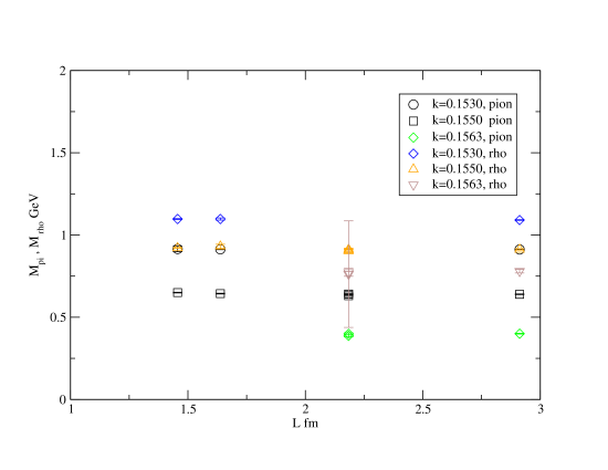
Figure 10: Dependence of the mass of the $\pi$ and $\rho$ mesons on the box size in quenched QCD for Wilson fermions at $\beta=6.0$. The data was taken from the compendium of World data in [199].

To get a more quantitative estimate of the volume dependence UKQCD [192] studied finite size effects in quenched QCD at $\beta=6.0$ with non-perturbatively improved clover fermions. Two volumes were used with sides 1.5 fm and 3 fm. For the pseudoscalar channel there was a $2\sigma$ difference between the mass on the two volumes. There were no statistically significant difference between the masses for the vector particle between the two lattice volumes.

To give some idea of the size of lattice spacing errors in the masses of the light mesons, I plot the mass of the $K^{\star}$ meson as a function of the lattice spacing in figure 11 from the CP-PACS collaboration [96]. The figure shows the difference between using the kaon or $\phi$ meson to determine the strange quark mass. The clear difference between the mass of the $K^{\star}$ when the strange quark mass is determined in two different ways is caused by the quenched QCD not being the theory of nature.

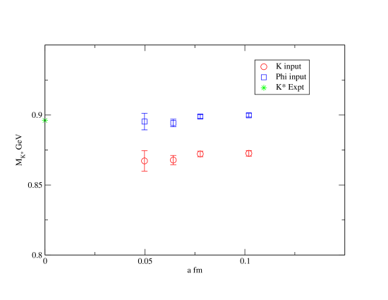
Figure 11: Lattice spacing dependence of the $K^{\star}$ meson in quenched QCD from the CP-PACS collaboration [96].

The results for meson masses in the continuum limit are in table [96].

Mass	Result ($m_{K}$ ) GeV	Result ($m_{\phi}$ ) GeV	Expt GeV
$m_{K}$	-	0.546(06)	0.496
$m_{K^{\star}}$	0.846(07)	0.891(05)	0.892
$m_{\phi}$	0.970(06)	-	1.020

Table 5: Masses of light S-wave mesons in quenched QCD from CP-PACS [96]. The different analyses depend on which meson is used to determine the strange quark mass.

The physical summary of the results in table 5 is that the hyperfine splitting is too low from quenched lattice QCD. To isolate the reduction of the hyperfine splitting, Michael and Lacock [174, 175] introduced the J parameter.

$$J=M_{V}\frac{dM_{V}}{dM_{P}^{2}}\mid_{M_{V}=1.8M_{P}}$$ (122)

where $M_{V}$ and $M_{P}$ are the vector and pseuodscalar masses respectively. The condition $M_{V}=1.8M_{P}$ corresponds to the experimental ratio of $K^{\star}$ and $K$ masses. This mass ratio was chosen so that an extrapolation to quark masses below strange was not required. Some theoretical problems with the value of $J$ defined at a light quark reference point are discussed by Leinweber et al. [157].

The J parameter has been chosen to be independent of the lattice spacing and a explicit definition of the quark mass. One experimental estimate for $J$ is obtained from

$$J=m_{K^{\star}}\frac{m_{K^{\star}}-m_{\rho}}{m_{K}^{2}-m_{\pi}^{2}}=0.48$$ (123)

Including the uncertainty from using $\phi-K^{\star}$ difference rather than the $K^{\star}-\rho$ mass difference, Michael and Lacock [174] estimate the experimental value of J to be $0.48(2)$.

In quenched QCD, Michael and Lacock [174] obtained $J=0.37(2)(4)$ in disagreement with the experimental estimate. Using their bigger data set, the CP-PACS collaboration [96] obtained J = 0.346(23) from a continuum extrapolation in quenched QCD.

The clear disagreement of the $J$ parameter from quenched QCD with experiment, in principle makes $J$ a good quantity to measure the effect of the sea quarks. The actual definition of J in equation 122 for unquenched QCD is not trivial because, as discussed in section 3.2, the lattice spacing does depend on the mass of the sea quarks. The issues in defining $J$ for unquenched QCD are discussed by the UKQCD collaboration [73].

Figure 12 compares the value of $J$ from the unquenched lattice QCD from UKQCD [73] and MILC [89].

Figure 12: Comparison of the J parameter from UKQCD [73] (diamonds) and MILC [89] (bursts). The experimental point is the square.

Both the calculations done by the UKQCD and MILC collaborations were at a fixed lattice spacing. The calculation by MILC was done at a lighter sea quark mass then UKQCD, that presumably explains why the value of J from MILC agrees better with the experimental value. The MILC result needs to be confirmed by a study of the lattice spacing dependence. Kaneko [31] has recently reviewed the status of calculations of $J$ from unquenched calculations.

The effect of unquenching on the hyperfine splitting in light mesons has an important effect on the value of the strange quark mass extracted from lattice data. For example, the CP-PACS collaboration [202] have used $n_{f}=2$ lattice QCD to calculate the strange quark mass. CP-PACS’s results are in table 6. The results show a sizable reduction in the mass of the strange quark between quenched and two flavour QCD. Lubicz [207] and Wittig [7] review the determination of the masses of quarks from lattice QCD.

$n_{f}$	input	$m_{s}$ MeV
2	$\phi$	$90^{+5}_{-11}$
2	$K$	$88^{+4}_{-6}$
0	$\phi$	$132^{+4}_{-6}$
0	$K$	$110^{+3}_{-4}$

Table 6: Mass of the strange quark from CP-PACS [202] in the $\overline{MS}$ scheme at a scale of 2 GeV.

6.1 P-WAVE MESONS AND HIGHER EXCITATIONS

The calculation of the masses of ground state mesons and baryons is essentially done to validate lattice QCD methods and to compute quark masses and the strong coupling. For excited S-wave and P-wave states, the issues are to determine the quark and glue content of the state (as well as to check that the masses agree with experiment). The signal to noise ratio is worse for P-wave mesons than for S-wave mesons [72], so the calculations are harder. These type of calculations tend to be more exploratory, so usually no attempt is made to take the continuum or infinite volume limit. As the underlying lattice techniques mature, there will be attempts quantify all the systematic errors.

The interpolating operators in table 4 can be used to create the P-wave $a_{0}$, $b_{1}$, and $a_{1}$ states. However, in the quark model these states have zero wave function at the origin. So non-local interpolating operators with a node at the origin have been tried [208, 209, 210]. Reasonable results can be obtained using the operators in table 4. Spin 2 states are not accessible from local interpolating operators, so must be created using non-local operators.

A more general approach [211] is to consider a generic non-local meson operator at a specific time $t$ (as is required for an interpolating operator for a time correlation function).

$$O(\underline{r})=\overline{\psi}(\underline{x},t)\Gamma\prod_{\underline{x},\underline{x}+\underline{r}}U\psi(\underline{x}+\underline{r},t)$$ (124)

where the quark and anti-quark are separated by a distance $\underline{r}$ and $\Gamma$ ia an arbitrary gamma matrix. The $\prod_{\underline{x},\underline{x}+\underline{r}}U$ is a set of gauge links that connects the quark to the anti-quark in a gauge invariant way. In general $\prod_{\underline{x},\underline{x}+\underline{r}}U$ is not unique and will effect the transformation properties of $O(\underline{r})$ under the cubic group. Operators are designed to transform under specific representations of the cubic group.

Continuum representation	cubic rep.
J=0	$A_{1}$
J=1	$T_{1}$
J=2	$E$,$T_{2}$
J=3	$A_{2}$,$T_{1}$,$T_{2}$
J=4	$A_{1}$,$E$ , $T_{1}$,$T_{2}$

Table 7: Representation of $SU(2)$ in terms of representations of the cubic group.

The connection between the representations of the cubic group and the $SU(2)$ rotation group are in table 7. The dimensions of the representations: $A_{1}$, $A_{2}$, $E$, $T_{1}$, $T_{2}$ are 1,1,2,3, and 3 respectively. Hence the dimensions of the representations match between the cubic group and $SU(2)$ rotation group with representation of $2J+1$ in table 7.

If the gauge configurations are fixed to Coulomb gauge then non-local interpolating operators based on spherical harmonics can be used. This approach was studied by DeGrand and Hecht [212, 72]. As hadron masses are gauge invariant quantities, gauge fixing at an intermediate stage should not effect the final results. Meyer and Teper discuss how to construct higher spin glueball operators [213].

There are number of interesting puzzles with the phenomenology of “P-wave” mesons. For example, there are speculations that the $a_{0}(980)$ particle is potentially not well described by a $\overline{q}q$ state in the quark model. Its mass is very close to the threshold for two kaon decay. There are many models that treat this state as a $\overline{K}K$ molecules [214] or $\overline{q}\overline{q}qq$ state. As lattice QCD calculations use the non-singlet $\overline{q}q$ operator to create this state, it may not couple strongly to a molecular $\overline{qq}qq$ state. Therefore I would expect that the lightest state in the $\overline{q}q$ channel to be the $a0$(1450). However, this speculation should, and will be [215] tested in unquenched lattice calculations.

As discussed in section 3.1, the interpretation of the $a_{0}$ state is complicated by a quenched chiral artifact [85] in quenched QCD. The largest systematic study of the $a_{0}$ in quenched QCD was done by Lee and Weingarten [86]. Unfortunately, they could only find the mass of the $a_{0}$ mass at the mass of the strange quark, possibly because of problems with the artifact in this channel. Alford and Jaffe [109] review some of the earlier results for the mass of the $a_{0}$ from quenched QCD. In a lattice calculation that used domain wall fermions and modelled the quenched chiral artifact, Prelovsek and Orginos [216] obtained the lightest state in the $a_{0}$ channel to be 1.04(7) GeV. At one coarse lattice spacing, Bardeen et al. [85] obtained a value of 1.34(9) GeV for the lightest state in the $a_{0}$ channel, also with an analysis that was aware of the quenched chiral artifact. The existing quenched lattice QCD data does not determine the mass of the lightest non-singlet $0^{++}$ state

In a two flavour unquenched calculation the UKQCD collaboration [215] quote the preliminary result for the mass of the $a_{0}$ to be 1.0(2) GeV at one lattice spacing. The MILC collaboration [89] have computed the $a_{0}$ mass with 2+1 flavours of sea quarks. The lightest mass of the $a_{0}$ in MILC’s calculation is 0.81 GeV [89]. The MILC collaboration [89] also claimed to see evidence for the open decay channels of the $a_{0}$ state. Hence, more work is required in unquenched QCD to determine the mass of the lightest non-singlet $0^{++}$ state.

The only values of the masses of the $a_{1}$ and $b_{1}$ mesons from unquenched QCD, I could find were from the MILC collaboration [89]. MILC obtained masses of the $a_{1}$ and $b_{1}$ of 1.23(2) and 1.30(2) GeV compared to the experimental values of 1.23(4) GeV and 1.2295(32) GeV respectively [6]. There doesn’t seem to be any interesting experimental issues with the $a_{1}$ and $b_{1}$ mesons. As noted by MILC [89], according to the quark model the masses of the $a_{1}$ and $b_{1}$ mesons should be similar to the mass of the $a_{0}$. Hence, any large splitting between the masses of $a_{0}$ and $a_{1}$ and $b_{1}$ is indicative of dynamics beyond the simple quark model.

The most surprising aspect of hadron spectroscopy are the existence of Regge trajectories. Empirically, the square of the mass of a hadron with mass $m(l)$ is linearly related to the spin by:

$$l=\alpha^{\prime}M^{2}(l)+\alpha(0)$$ (125)

Although the Regge trajectories can be explained by models (see [217] for a review), in particular the string model, the existence of Regge trajectories has not been shown to be a rigorous consequence of QCD. Equation 125 is a very useful tool in classifying baryon states. Historically some of the spin assignments of baryons were guessed from equation 125 [218]. Equation 125 is also useful in scattering experiments (see [219] for a discussion).

The simple relation in equation 125 has recently been challenged by a number of authors. The improved precision of the experimental data on hadron masses has allowed fits to the spectrum that seem to show some nonlinearity in the relation between the square of the meson masses and their spin [220]. Brisudova et al. [221] discuss various hadronic models that can reproduce linear and nonlinear Regge trajectories. The nonlinearities in the Regge trajectories were related to flux tube breaking [217], hence the study of Regge trajectories is complimentary to the study of string breaking [222]. Brisudova et al. [217] make the prediction that are no light quark quarkonia beyond 3.2 GeV due to the termination of the Regge trajectories. If this conjecture is correct, then this might simply searches for hybrid and glueballs in the region from 3 to 5 GeV.

The problem for lattice QCD calculations is that it is hard to construct interpolating operators with spin higher than 2 on the lattice. As higher orbital states have larger masses than ground state mesons, they have a worse signal to noise ratio, so it is hard to extract a signal from the calculations.

There have been some calculations of spin 3 masses from lattice QCD calculations. The UKQCD collaboration [211] studied spin 2 and spin 3 states in a quenched lattice QCD calculation, In figure 13, I plot their results in a Chew-Frautschi plot [223] with experimental data from the particle data table.

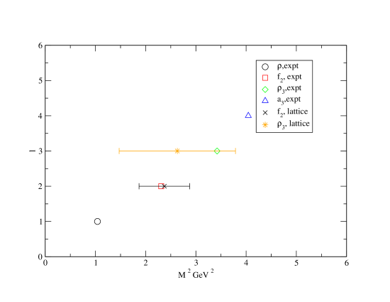
Figure 13: Square of the mass of the meson mass versus its spin $l$. The octagons are the experimental numbers and the bursts are the lattice QCD data from UKQCD [211]. The quarks have the mass of the strange quark. There are only error bars on the lattice data.

There have been a few attempts to study the spectroscopy of excited mesons using lattice QCD. As discussed in section 2 the computation of the masses of excited states requires a multi-exponential fit to the lattice correlators that can be unstable.

The CP-PACS collaboration [79] used the maximum entropy method (briefly revived in section 2) to study the excited spectrum of the rho and pion mesons. The calculations were done in quenched QCD, using the same data set that was used for their calculation of the ground state masses [196].

A spectral density from CP-PACS [79] is in figure 14. The masses of the states are obtained from the peaks in figure 14.

Figure 14: Spectral function (from MEM) from the CP-PACS collaboration for the $\rho$ correlators. The lattice spacing is $a^{-1}$ = 2.58 GeV. The K11, K42, and K44 keys are the plots for mesons with different quark masses.

Figure 15 from CP-PACS [79] shows the masses of the excited $\rho$ meson as a function of lattice spacing. The diverging graph in figure 15 is thought to be a bound state of fermion doublers.

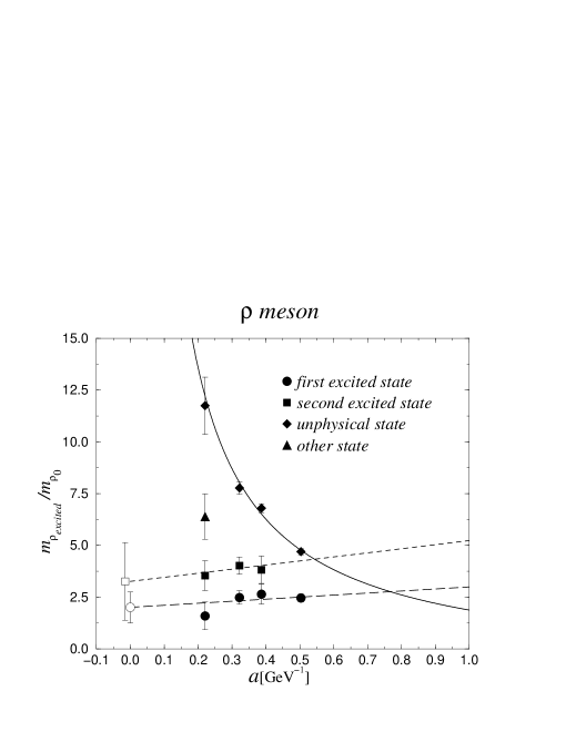
Figure 15: Continuum extrapolation of the masses in the vector channel from CP-PACS.

The final results from CP-PACS [79] were that the first excited state of the pion had a mass of 660(590) MeV and the mass of the first excited rho meon was 1540 (570) MeV from quenched QCD. The errors also include an estimate of the error from taking the continuum limit.

Experimentally [6], the first excited pion is the $\pi(1300)$ with the mass of $1300\pm 100$ MeV. The excited states of the $\rho$ meson are more interesting. There are two states: $\rho(1459)$ with a mass of $1465\pm 25$ and the $\rho(1700)$ with a mass of $1700\pm 20$ MeV. Donnachie [224] reviews the evidence for a hybrid state in the $1^{--}$ channel.

The errors on the excited states from CP-PACS are really too big for a meaningful comparison with experiment. The results from CP-PACS [79] need confirmation from other, less Bayesian based fitting methods, such as variational methods.

7 THE MASSES OF LIGHT BARYONS

An important, but perhaps slightly boring, goal of lattice QCD is to compute the mass of the nucleon with reliable errors from first principles. The nucleon is the most important hadron for the real world of the general public, but the nucleon’s role in the esoteric domain of particle physics is as “background” to the more interesting stuff. In this section, I will discuss the highlights of some recent large scale quenched and unquenched QCD calculations. As the aim of lattice QCD calculations for these baryons is to validate lattice QCD before the spectroscopy of more interesting hadrons is attempted, the focus will be on the error analysis.

In principle the mass of the nucleon should be an ideal quantity to compute on the lattice, because it is stable within QCD, hence there are no concerns with the formalism due to decay widths. The main complication with getting an accurate value of the nucleon mass is the large chiral extrapolation required (see section 3.3) caused by the large quark masses used in the calculations. In the majority of lattice QCD calculations, electromagnetism is ignored, so I refer to the generic nucleon rather than the neutron or proton.

The “standard” interpolating operators for the nucleon [16, 225]

$$N_{1}^{1/2+} = \epsilon_{ijk}(u_{i}^{T}C\gamma_{5}d_{j})u_{k}$$

$$N_{2}^{1/2+} = \epsilon_{ijk}(u_{i}^{T}Cd_{j})\gamma_{5}u_{k}$$

where $u$ and $d$ are operators that create the up and down quark respectively and $C$ is the charge conjugation matrix. In the non-relativistic limit (keeping the upper components) the $N_{2}$ operator vanishes, so it doesn’t couple strongly to the nucleon. Empirically the $N_{2}$ operator has been found useful for $N^{\star}$ states. Leinweber [226] discusses the connection between the interpolating operators for the nucleon used on the lattice and those used in QCD sun rules.

The nucleon correlator is constructed, in the standard way, by creating a nucleon at the origin, and then destroying it at time t later.

$$C_{\pm}(t)=\sum_{\underline{x}}\langle 0\mid N(\underline{x},t)(1\pm\gamma_{4})\overline{N}(\underline{0},0)\mid 0\rangle$$

The specific representation of equation 23) is slightly more subtle.

$$C_{+}(t) \rightarrow A^{+}e^{-m_{+}t}+A^{-}e^{-m_{-}(T-t)}$$

$$C_{-}(t) \rightarrow A^{-}e^{-m_{-}t}+A^{+}e^{-m_{+}(T-t)}$$

where $m_{+}$ and $m_{-}$ are the masses of the lightest positive and negative parity states.

To illustrate the finite size effects on the mass of the nucleon in quenched QCD, I plot the nucleon mass as a function of box size for Wilson fermions at $\beta=6.0$ in figure 16. This data set was chosen because there was data at a number of different volumes. For all the data I used the lattice spacing of a= 0.091 fm [195]. The dependence of the nucleon mass on the length of the lattice looks “mild” from figure 16. Unfortunately. the statistical errors on the lightest data are too large to make any statement about finite size effects.

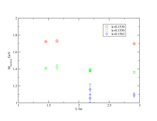
Figure 16: Dependence of the mass of the nucleon on the box size in quenched QCD for Wilson fermions at $\beta=6.0$. The data was taken from the compendium of World data in [199].

For many years, the quality of a lattice QCD calculations was judged by the final value of ratio of the nucleon mass to rho mass. I now discuss some recent quenched QCD calculations in more detail.

There was a large scale calculation of the quenched QCD spectrum by the MILC collaboration [227] that used staggered fermions. The study included four different lattice spacings: $a^{-1}$ from 0.63 to 2.38 GeV and also investigated finite size effects.

The MILC collaboration [227] tested 12 different chiral extrapolation models based on generic model for the dependence of a hadron mass $M_{H}$ on the quark mass $m_{q}$.

$$M_{H}=M+am_{q}^{1/2}+bm_{q}+cm_{q}^{3/2}+dm_{q}^{2}+em_{q}^{2}\log m_{q}$$ (126)

Only three of the fit parameters (a,b,c,d,e) were varied in a fit model. The fit model in equation 126 was broad enough to include both full and quenched chiral perturbation theory. It is important to test more than the quenched chiral perturbation theory results, because it is not clear that the data is in the regime where the expressions are valid are valid. The simple linear fit, where only $b$ was non-zero in equation 126, was not consistent with the data [227].

The MILC collaboration found that the coefficient of the $m_{q}^{1/2}$ term from their fits was the wrong sign from the expectations from quenched chiral perturbation theory, hence this term was not included in the their final fits. For the $\rho$ extrapolation the coefficient of the $m_{q}^{3/2}$ term was an order of magnitude lower than expected The analysis of the chiral extrapolations was complicated by the flavour symmetry breaking terms of staggered fermions [227]. This seems to be a perennial feature of the staggered fermion formalism [228].

The result from the MILC collaboration [227] for the ratio of the nucleon to rho mass ratio was $m_{N}/m_{\rho}$ = $1.254\pm 0.018\pm 0.027$, where the first error is statistical and the second error is systematic (in the summary figure 17) I have added the two errors in quadrature).

Kim and Ohta [229] studied quenched QCD using staggered fermion with a smaller lattice spacig ($a^{-1}$ = $3.63\pm 0.06$ GeV) and lighter quarks than were used by the MILC collaboration [227]. The spatial length was $2.59\pm 0.05fm$ and their lightest quark mass was 4.5 MeV. They fitted the same chiral extrapolation models as MILC [227] did, but also had problems unambiguously detecting the predictions from quenched chiral perturbation theory. Kim and Ohta also studied some chiral extrapolation formulae, suggested by [230], that looked for finite volume effects masquerading as quenched chiral logs. Kim and Ohta’s result [229] was $m_{N}/m_{\rho}$ = $1.24\pm 0.04(stat)\pm 0.02(sys)$

The CP-PACS collaboration [96] found $m_{N}/m_{\rho}$ = 1.143 (33)(18). In the fits of the vector particle as a function of the quark mass, CP-PACS excluded the $m_{q}^{3/2}$ term, but included the $m_{q}^{1/2}$ term The coefficient of the $m_{q}^{1/2}$ term was found to be an order of magnitude less than the naive expectation.

In figure 17, I plot the results for the ratio of the nucleon and rho masses from some recent quenched lattice QCD calculations [4, 96, 227, 192]. I have selected calculations where an attempt was made to take the continuum limit. For comparison, in the strong coupling limit $g\rightarrow\infty$ the hadron spectrum can be computed analytically. In this limit the ratio of the nucleon and rho masses is $\frac{m_{N}}{m_{\rho}}=$ 1.7 [18]

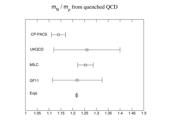
Figure 17: The ratio of the nucleon mass to rho mass from several recent large scale quenched QCD calculations. ( [4, 96, 227, 192]. ).

The agreement with experiment for the $m_{N}/m_{\rho}$ ratio from quenched QCD is surprisingly good. Although agreement at the 10 % level may sound quite impressive, errors of this magnitude are too large for QCD matrix elements required in determining CKM matrix elements from experiment [5]. The analysis of Booth et al. [152] using the non-analytical terms from quenched chiral perturbation theory estimated that the value of $m_{N}/m_{\rho}$ from quenched QCD could be as low as 1.0. This situation is not seen in the lattice results, however none of the quenched QCD calculations have detected the predicted dependence of the mass of the $\rho$ meson on the quark mass, To confirm the quark mass dependence predicted by quenched chiral perturbation theory requires new calculations with lighter quarks. The QCDSF collaboration [231] obtained a coefficient of the $m_{q}^{1/2}$ term from their fits that was roughly in agreement with expectations from quenched chiral perturbation theory.

A summary of some of the hadron spectrum from quenched QCD from the work by CP-PACS [96] is shown in figure 18.

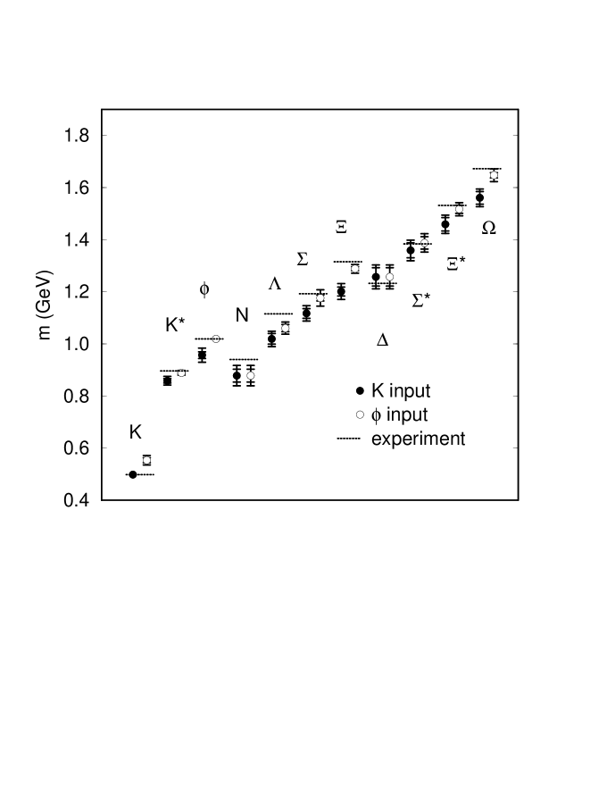
Figure 18: Final results for the light hadron spectrum from CP-PACS in quenched QCD [96].

The ALPHA collaboration notice that the largest deviations from experiment of the quenched lattice results from CP-PACS are for resonant hadrons [182] if the lattice spacing is determined from the nucleon mass. The BGR collaboration also note a similar trend in their data [197]. This trend could be modelled using techniques similar to those used by Leinweber and Cohen [155] to study the $\rho$ meson. It is difficult to see from figure 18 that the hadrons with large widths have masses in quenched QCD that differ more from experiment than those with smaller widths.

As discussed by Aoki [29] and the CP-PACS collaboration [96] the value of the mass of the nucleon from CP-PACS [96] and MILC [227] differ at the $2.5\sigma$ level. The two calculations used different fermion formulations, each with a different set of potential theoretical problems, that should in principle produce the same results in the continuum limit.

The main criticisms of the CP-PACS quenched study are on their treatment of the quenched chiral perturbation theory. Wittig reviews the lattice results for detecting the quenched chiral log [7]. The new calculations that use light fermion actions with better chiral symmetry properties are disagreeing with the result from CP-PACS. These new calculations are done at a fixed (small volume) and large lattice spacings, so perhaps there are systematic errors in their results [7]. The CP-PACS and MILC collaborations used the mass of the $\rho$ to determine the lattice spacing. It would have been interesting to see the dependence of the final results on using different quantities to determine the lattice spacing.

Although it may be possible to do a more systematic study of quenched QCD at lighter quark masses than CP-PACS [196], I am not sure that it is worth it. As discussed in section 3.3 the crucial non-analytic terms in quenched and unquenched chiral perturbation theory are very different, so calculations with light quarks in quenched QCD will have very little direct relevance for unquenched calculations. As the masses of the quarks in unquenched calculations decrease we should start to see the effect of the decay of the hadrons. The effect of particle decay on the mass spectrum can not be studied in quenched QCD.

I will now describe the results from recent unquenched lattice QCD calculations. As usual the systematic errors must first be discussed. There have been two recent studies of finite size effects in the nucleon from unquenched QCD, carried out by the JLQCD [232] and UKQCD [111]. The results are plotted in figure 19.

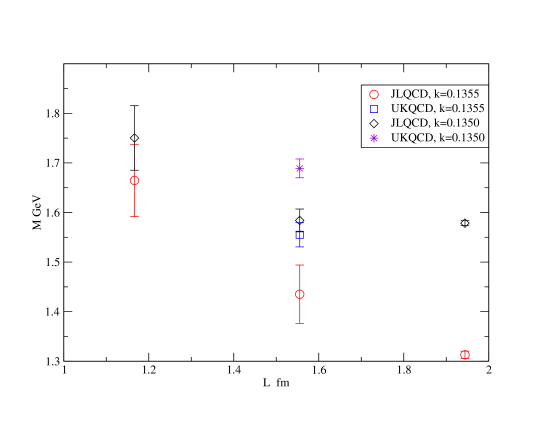
Figure 19: Dependence of the mass of the nucleon on the box size from UKQCD [111] and JLQCD [232]. These are two flavour unquenched calculations.

One slight concern with the nice study of finite size effects from JLQCD [232] is the large statistical errors on the two smaller volumes. Also there is some disagreement between the results from UKQCD and JLQCD on the $16^{3}$ volume. As stressed by the MILC collaboration [83] a careful control of statistical errors is required to see definitive evidence for the effect of the box size on the masses of hadrons.

In figure 20 I plot the dependence of some hadron masses on the lattice spacing from the calculations by the CP-PACS collaboration [96]. This should give some idea of the size of the lattice spacing errors in unquenched QCD.

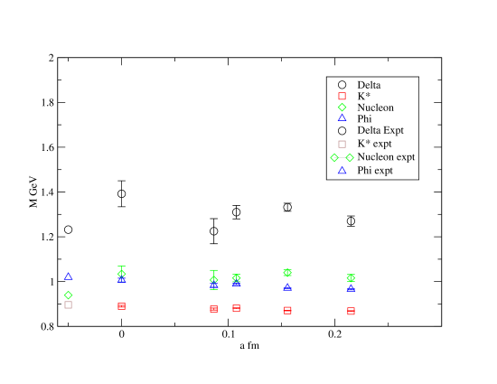
Figure 20: Dependence of hadron masses on the lattice spacing. from CP-PACS [96] in 2 flavour unquenched QCD. Data from the finest lattice spacing was not used in the continuum extrapolation.

As discussed in section 6 the main “successes” of unquenching have occurred in the meson sector. A detailed comparison of the baryon spectrum with experiment is obscured by lattice spacing and finite size effects [134, 232]. In a preliminary analysis the MILC collaboration [233] found that $m_{M}/m_{\rho}$ from two flavour unquenched QCD in the continuum limit was higher than the value in the quenched QCD, so the quenched value agreed better with experiment than the unquenched result. The MILC collaboration [89] are now studying this issue using a better version of staggered fermions with 2+1 unquenched flavours.

In table 8, I compare the results from lattice QCD with the old results from the Isgur-Karl quark model [234]. Although the Isgur-Karl model agrees better with experiment than the two lattice QCD calculations, because the lattice QCD calculations are based on the QCD Lagrangian, the hadron masses can be used to extract quark masses. This is not possible from quark models where there is no way of relating the constituent quark masses to the masses in the Lagrangian. The more interesting tests of the quark model occur for excited baryons. I discuss the lattice results for these hadrons in section 7.1.

In fact the agreement between the hadron masses from the quark model and experiment is actually too good. The quark model calculation of Isgur and Karl [234] does not include the dynamics of hadron decay. For example the $\Delta$ baryons have decay widths of around 120 MeV [6]. It might have been expected that the errors in the quark model predictions for the hadron masses would be of the order of the decay width. Isgur and Geiger [156, 235] have developed a formalism to absorb some of the effects of quark-antiquark loops into the potential. This issue is also reviewed by Capstick and Roberts [236]..

Baryon	Expt.	Isgur-Karl MeV	CP-PACS (quenched)	CP-PACS (unquenched)
$N$	940	940	878(25)	1034(36)
$\Lambda$	1116	1110	1019(20)	1160(32)
$\Sigma$	1193	1190	1117(19)	1202(30)
$\Xi$	1315	1325	1201(17)	1302(28)
$\Delta$	1232	1240	1257(35)	1392(58)
$\Sigma^{\star}$	1384	1390	1359(29)	1488(49)
$\Xi^{\star}$	1532	1530	1459(26)	1583(44)
$\Omega$	1673	1675	1561(24)	1680(41)

Table 8: Comparison of the hadron masses from unquenched and quenched lattice QCD calculations with the results from the Isgur-Karl quark model [234]. The unquenched data is taken from CP-PACS [134]. The quenched data is also from CP-PACS [196]. For the lattice results the strange quark mass is set by the kaon mass.

7.1 EXCITED BARYON STATES

Recently there has been a lot of work on the spectroscopy of excited nucleon states from lattice QCD. This research is mostly motivated by the experimental program at the Jefferson lab [13, 14, 15] The accurate spectroscopy of the $N^{\star}$ states will be an accurate test of our understanding of the forces and effective degrees of freedom in hadrons [237]. Realistically, lattice QCD calculations may only be able to obtain one or two excited baryon states from a specific channel. However this is enough to (potentially) solve some very interesting and long standing puzzles.

At the moment the identification of the Roper resonance from lattice QCD is controversial, so I will introduce some notation to prevent ambiguity. I call the nucleon the $N$ state, the first excited nucleon with positive parity the $N^{\prime}$ state, and the first excited nucleon with negative parity the $N^{\star}$ state. In the particle data table, the $N^{\prime}$ state would be the $N(1440)$ and the $N^{\star}$ state would be the $N(1535)$.

There is a potential artifact associated with quenched QCD for baryon states [238, 239]. The mass of the $\eta^{\prime}N$ state is experimentally close to the mass of the $N(1440)$ and $N(1535)$ states. In quenched QCD the $\eta^{\prime}$ is treated incorrectly, so the intermediate $\eta^{\prime}N$ state is also incorrect. This is the analogue of the artifact in the scalar correlator found by Bardeen at al. [85] discussed in section 3.1. Dong et al. [240] claim to have seen the correlator, that would be positive definite in unquenched QCD, for the $N^{\star}$ state go negative for pion masses below 248 MeV. If this artifact causes the correlator to go negative this may “confuse” fitting techniques such as the maximum entropy method that relies on a positive definite correlator. There is no chiral artifact in unquenched QCD. Work has started on studying the Roper resonance using unquenched QCD [241].

In table 9 I have collected some results for the ratio of the $N^{\star}$ mass to the nucleon mass from some recent quenched lattice QCD calculations. Only the calculation by Gockeler et al. [239] took the continuum limit. The experimental number corresponds to the mass of the $N(1535)$ divided by the nucleon mass about: 1.63. It is not clear what effect the 150 MeV width of the $N(1535)$ will be on the lattice result.

Reference	Comments	$M_{N^{\star}}/M_{N}$
Blum et al. [242]	Domain wall	$1.49(9)$
Gockeler et al. [239]	Clover	$1.50(3)$
Broemmel et al. [243]	Overlap	$1.77(7)$
Dong et al. [240]	Overlap	$1.67(12)$
Nemoto et al. [244]	anisotropic clover	$1.463(51)$

Table 9: Ratio of the mass of the parity partner of the nucleon to the nucleon mass from the quenched QCD.

The nature of the Roper resonance ($N(1440)$) is still a mystery. There is an experimental signal for this state, but it is not clear what the quark and glue composition of this hadron is. On the lattice three quark interpolating operators are used to study the Roper state. If the mass of the Roper is not reproduced, then this would be evidence that additional dynamics, beyond three valence quarks, is important for this state.

The quark model has problems reproducing the experimental mass of the Roper resonance. Using a simple harmonic oscillator potential to study the hadron spectrum, Isgur and Karl [242, 245] used a oscillator quantum of 250 MeV. In quark model language, the $N^{\star}$ state would have one quantum above the ground state, and the $N^{\prime}$ state would have two quantums above the ground state. This predicted ordering is opposite to the experimental masses of the $N(1440)$ and $N(1535)$. Capstick and Roberts review the nature of the Roper resonance in the context of potential models [236]. Isgur also discusses the problems of the Roper resonance in the quark model. [237]. The predictions of the quark model for the lowest excitations of the nucleon improve if a more realistic potential is used, and the mixing between states is taken into account [236, 237].

There are predictions from flux tube and bag models that the lightest hybrid baryon (three quarks with excited glue) [246, 247] is $J^{P}=1^{+}$ with a mass in the region 1.5 to 1.9 GeV, hence close to the mass of the Roper resonance.

Sasaki, Blum, and Ohta [242] studied the first excited state of the nucleon at a fixed lattice spacing of 0.1 fm and with a physical length of the lattice as 1.7 fm. Their calculations were done in quenched QCD with quark mass in the range $M_{PS}/M_{V}$ 0.59 to 0.9. The excited state masses were extracted using a variational technique with two basis states that were different interpolating operators for the nucleon. Sasaki et al [242] could only obtain a signal for the $N^{\prime}$ state for pion masses above 600 MeV. The mass of the $N^{\prime}$ state was larger than the $N^{\star}$ state. If the variational technique was not biased by truncation of the sum of excited states, then the calculation of Sasaki [242] should be able to resolve the ground and first excited states. For the negative parity states, the masses obtained from the ground and first excited state were degenerate. This could be interpreted as the variational technique not being able to resolve two states. Experimentally the lightest $N^{\star}$ states are the $N(1535)$ and $N(1650)$.

Melnitchouk et al. [248] have also studied the spectrum the masses of the $N$, $N^{\star}$, and $N^{\prime}$ states. Their raw data for the splitting between the $N$ and $N^{\star}$ states is consistent with other groups [242, 239]. The mass for the $N^{\prime}$ state was much higher than the mass of the experimental Roper resonance.

Dong at al. [240] claim agreement between the mass of the $N^{\prime}$ state from their calculation and the mass of the Roper resonance from experiment. The calculation was done with the lattice spacing of 0.2 fm and a physical box lengths of 2.4 and 3.2 fm. The calculations used very light valence quarks (for the lattice anyway). The lightest pion mass was 180 MeV. The excited state masses were extracted using the constrained curve fitting method developed from the proposal by Lepage at al. [64]. Dong at al. [240] reported that the mass of the $N^{\prime}$ state started to decrease rapidly with pion masses below 400 MeV. The mass of the $N^{\prime}$ state was less than that of the $N^{\star}$ state for pion mass of about 220 MeV. The mass quoted for the $N^{\prime}$ state is 1462(157) MeV. The large error bars on this result means that a 2 $\sigma$ statistical fluctuation would give 1776 MeV.

Sasaki [249] has reported a study of the finite size effects on the mass of the excited state of the nucleon. The excited state of the nucleon was studied at the fixed lattice spacing of 0.09 fm. Three physical box sizes were used: 1.5 fm, 2.2 fm and 3.0 fm. The mass of the $N^{\prime}$ state was extracted using the maximum entropy method. The $N^{\prime}$ and $N$ states had finite size effects that increased as the light quark masses were reduced. The final result for the $N^{\prime}$ state looks as though it would extrapolate to the experimental value from pion masses around 600 MeV. No dramatic decrease in the mass of the $N^{\prime}$ is required. The picture from the calculation of Sasaki [249] disagrees with that from Dong et al. [240].

Broemmel et al [243] have tried to study the Roper resonance using lattice QCD. They used an overlap-Dirac fermion operator with a lattice spacing of 0.15 fm and two physical lattice sizes of 1.8 and 2.4 fm. To study excited states they used a variational technique based on three interpolating operators. They could get a signal for the nucleon with pion masses as low as 220 MeV. Unfortunately, they could extract a signal for excited nucleon states with pion masses above about 550 MeV. This stopped them being able to confirm the mass dependence of the $N^{\prime}$ state claimed by Dong et al. [240]. This analysis did not include the effect of the quenched chiral artifact in this channel. Broemmel et al [243] extracted both the ground and first excited state of the negative parity nucleon channel.

From the very interesting recent studies [242, 240, 249, 243] of the Roper resonance on the lattice it is clear that careful attention will have to be paid to the systematic errors. Pion masses below 200 MeV may be required. It would be good to have variational calculations with wider sets of interpolating operators as a check on the various Bayesian based fitting techniques. For example it would be reasonable for “fuzzed“ nucleon operators [46] to couple more to hybrid baryon states because they contain more glue. It is a high priority that other groups try to reproduce the results of Dong at al. [240]. and Sasaki [249].

One particular concern with getting the mass of the $N(1440)$ is that its width is 380 MeV. The decay of $N(1440)$ will effect its mass. This is also a difficulty for potential model calculations. Capstick and Roberts [236] estimate that ignoring the width of the $N(1440)$ causes an uncertainty of the order of 100 MeV on the mass within the potential model framework.

Although I have focused on the excited states of the nucleon, there is growing body of work on the parity partners of other baryons [244, 248].

8 ELECTROMAGNETIC EFFECTS

The majority of lattice QCD calculations do not incorporate the effect of the electromagnetic fields in hadron mass calculations. This is reasonable, because the dominant interaction for hadron masses is the strong force. I review the work done on including electromagnetic fields in lattice QCD calculations.

The theory of QED has been studied by many groups using lattice techniques. The formalism is similar to that discussed in section 2, except that the gauge group is U(1). However, there are some conceptual differences, because the U(1) gauge theory is not asymptotically free. Issues relating to the non-asymptotically free nature of QED have been studied in a non-perturbative way on the lattice [250, 251]. Also there are compact and non-compact versions of the lattice $U(1)$ theory. In non-compact QED the gauge fields $A_{\mu}^{em}$ take to the range $-\infty$ to $\infty$.

To study electromagnetic effects on the hadron spectrum the electromagnetic fields have been quenched. The dynamics of the sea quarks have not been included in the generation of the U(1) gauge fields. A comparison between the use of background fields in sum rules and lattice QCD has been made by Burkardt et al. [252].

The most “comprehensive” study of the effect of electromagnetism on the masses of hadrons has been performed by Duncan et al. [253, 254]. They used a non-compact version of QED The gauge fields were generated using the action

$$S_{em}=\frac{1}{4e^{2}}\sum_{x}\sum_{\nu\mu}(D_{\mu}A_{\nu}(x)-D_{\nu}A_{\mu}(x))$$ (127)

where $e$ is the electromagnetic charge. The $A_{\mu}(x)$ fields were subject to the linear Coulomb condition. The fields were promoted to compact fields $U(x)_{\mu}=e^{\pm iqA_{\mu}(x)}$. This field coupled to a quark field with charge $\pm qe$.

Currently, lattice QCD calculations are usually not accurate to 10 MeV, the order of magnitude of electromagnetic effects on the masses of light hadrons. To increase the mass splitting Duncan et al. [253, 254] used large charges (2 to 6 times the physical values) and then matched onto chiral perturbation theory that included the photon field.

The chiral extrapolation fit model used for pseudoscalars with electromagnetic fields

$$m_{P}^{2}=A(e_{q},e_{\overline{q}})+m_{q}B(e_{q},e_{\overline{q}})+m_{\overline{q}}B(e_{q},e_{\overline{q}})$$ (128)

where $e_{q}$, $e_{\overline{q}}$ ($m_{q}$, $m_{\overline{q}}$) are the (masses) of the quark and anti-quark

The calculations of Duncan et al. [253, 254] were done with one coarse lattice spacing $a^{-1}\sim 1.15$ GeV with a box size of 2 fm. Some of the results for the mass splittings from Duncan et al. are in table 10. I have included both the data and the corrected results, where theoretical expressions were used to correct for finite volume effects.

Mass splitting	Raw Lattice QCD (MeV)	Corrected MeV	Experiment (MeV)
$m_{\pi^{+}}-m_{\pi{-}}$	4.9(3)	5.2(3)	4.594)
$m_{n}$ - $m_{p}$	2.83(56)	1.55(56)	1.293
$m_{\Sigma^{0}}-m_{\Sigma^{+}}$	3.43(39)	2.47(39)	3.27
$m_{\Sigma^{-}}-m_{\Sigma^{0}}$	4.04(36)	4.63(36)	4.81
$m_{\Xi^{-}}-m_{\Xi^{0}}$	4.72(24)	5.68(24)	6.48

Table 10: Electromagnetic mass splittings from Duncan at al. [253, 254]

There has some work on computing electromagnetic polarizabilities [255, 256, 257] from lattice QCD. The electric ($E$) and magnetic ($B$) polarizabilities measure the interaction of a hadron with constant electromagnetic fields. Under the electromagnetic field the mass of the hadron is shifted by $\delta m$.

$$\delta m=-\frac{1}{2}\alpha E^{2}+-\frac{1}{2}\alpha B^{2}$$ (129)

The $\alpha$ and $\beta$ quantities should be computable from QCD. Holstein [258] reviews the theory and experiments behind the nucleon polarizabilities. The experimental values for $\alpha$ and $\beta$ are extracted from Compton scattering experiments (see  [259] for example3). A comparison of the results from lattice QCD to models and experiment can be found in two recent papers [256, 257].

In contrast to work of Duncan et al. the formalism used for electromagnetic polarizations [255] uses static electromagnetic fields. The $SU(3)$ gauge fields are modified by multiplying

$$U_{1}(x)\rightarrow e^{i\alpha qEx_{4}}U_{1}(x)$$ (130)

where $x_{4}$ is the Euclidean time variable and $E$ is the constant electric field. The phase factor in equation 130 can be linearised. Smit and Vink have described how to put a constant magnetic field on the lattice [260].

There are speculations that in very strong magnetic fields ($B\geq 5\times 10^{14}$ T), the proton will become unstable to the decay to neutrons [261]. Magnetic fields of this intensity may be realised in the universe [262]. The original estimate [261] of the instability of the proton was done in the quark model. In an attempt to remove some of the uncertainty in the hadronic calculation, Rubinstein et al. [263] used lattice QCD to study the dependence of the masses of the proton and neutron on the magnetic field.

Some early lattice calculations included the magnetic fields to look at the magnetic moments of hadrons [264, 265]. However, it is best to calculate magnetic moments from form factors [266, 267, 268], so electromagnetic fields are no longer used.

Electric fields were used in the first (unsuccessfully) attempts to compute the electric dipole moment of the neutron [269, 270]. The calculation of the neutron electric dipole moment has recently been reformulated [271] in a way that does not require the use of electromagnetic fields.

9 INSIGHT FROM LATTICE QCD CALCULATIONS

The start of the book Numerical Methods for Scientists and Engineers by Hamming has the immortal phrase: “the purpose of computing is insight not numbers.” In the previous sections I have described how lattice QCD is used to compute the masses of hadrons. This may give the impression that lattice QCD is essentially just a black box that produces the masses of hadrons without any insight into the physical mechanisms or relevant degrees of freedom. In this section I hope to show that lattice QCD can also help to explain the physical mechanisms behind the hadron mass spectrum. A very good overview of the type of insight wanted from hadronic physics, that contrasts the hadron spectroscopy approach to the study of confinement with the results from DIS type studies, is the paper by Capstick et al. [272]. Note however for the B physics experimental program, high precision numbers with reliable error bars are required to look for evidence for physics beyond the standard model of particle physics [273].

Isgur’s motivation [237] for studying the $N^{\star}$ particles is based on trying to understand the important degrees of freedom that describe low energy QCD. Increasingly, lattice QCD calculations are being used to provide insight into the dynamics of QCD. Some of Isgur’s last papers [274, 275, 105, 106] were devoted to using lattice QCD to validate the quark model picture of hadronic physics.

At first sight the model building approach to studying QCD appears to give more insight into the dynamics of QCD. It is usually quite easy to study the effect of adding new interactions to the model. There are many models for QCD interactions: quark model [236], instanton liquid model [276], or bag model [277]. The main problem with the model based approach to hadron spectroscopy is that is very difficult to judge whether the assumptions in the models are valid. The models are only believed when they provide a reasonable description of “most” experimental data with a good $\chi^{2}$, but this does not prove that they are correct. Different models of the QCD dynamics can be based on very different physical pictures, but may give equally valid descriptions of experimental data. For example the physical assumptions behind the bag model seem to be very different to the assumptions behind the instanton liquid model [276]. The major advantage of lattice QCD calculations is that the theory can be mutilated in a controllable way, so the physical mechanism underlying a process can be studied.

For example, the question about what mechanism in QCD causes a linearly rising potential for heavy quarks at intermediate distances is not something that can be answered by the quark model. Greensite [278] reviews the work on studying “confinement” using lattice QCD).

In this section I will focus on various attempts to explain the value of the mass splitting between the nucleon and delta. According to the quark model [6], the masses of the nucleon and delta are split by a spin-spin hyperfine term:

$$H_{HF}=-\alpha_{S}M\sum_{i>j}(\vec{\sigma}\lambda_{a})_{i}(\vec{\sigma}\lambda_{a})_{j}$$ (131)

where the sum runs over the constituent quarks and $\lambda_{a}$ is the set of SU(3) unitary spin matrices (a runs from 1 to 8). In perturbative QCD a term of the form 131 is naturally generated, but it is not clear whether the equation 131 is relevant for light relativistic quarks.

Lattice QCD calculations can produce more masses than experiment, so the hyperfine interaction can be tested [279, 280]. A pictorial measure of the quark mass dependence of the masses of the octet and decuplet is given by the “Edinburgh” plot from CP-PACS [96] is in figure 21.

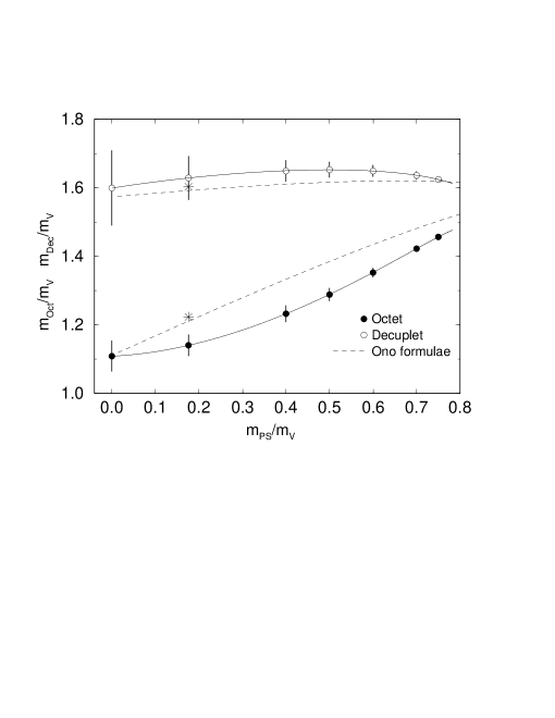
Figure 21: Edinburgh plot from CP-PACS [96] from quenched QCD. The lattice data is compared against the quark model of Ono [281].

The continuous curve is from a quark model by Ono [281] that uses:

$$M_{baryon} = M_{b}+\sum_{i}m_{i}+\xi_{b}\sum_{i>j}\frac{\vec{S_{i}}\vec{S_{j}}}{m_{i}m_{j}}$$

$$M_{meson} = M_{m}+\sum_{i}m_{i}+\xi_{b}\sum_{i>j}\frac{\vec{S_{i}}\vec{S_{j}}}{m_{i}m_{j}}$$ (132)

The agreement between the lattice data and Ono’s model is reasonable in figure 132. The lattice QCD data from CP-PACS [96] in figure 21 is almost precise enough to show deviations from the model by Ono [281] (equation 132).

In the instanton liquid model [101], the vacuum is made up of a liquid of interacting instantons. There has been a lot of work on comparing the instanton liquid model against lattice QCD. The basic idea is to cool the gauge configuration [51]. This removes the perturbative part of the gauge field and leaves the classical configurations, that can be compared against the predictions of the instanton liquid model. The cooling procedure is essentially a way of smoothing the perturbative noise from the configurations. This perturbative noise presumably has something to do with the one gluon exchange term.

In the first study of this on the lattice [282], the masses of the nucleon, $\rho$, $\Delta$ and $\pi$ were measured in the usual way. The gauge configurations were then cooled and the simple hadron spectrum was measured again. The masses for the $\rho$ $\pi$ and nucleon particles were qualitatively the same before and after cooling. As the cooling does not effect the instantons this suggested that the mass splittings are largely due to instantons. The mass splitting between the nucleon and $\Delta$ was reduced by smoothing. Chu et al. [282] claimed that this was due to the problems with extracting the mass of the $\Delta$ from the lattice data. Later work on this issue [283, 100] has not returned to the effect of instantons on the mass splitting between the nucleon and $\Delta$. Rosner and Shuryak [284] have shown that simple instanton interactions can give a reasonable representation of some baryon mass splittings.

In a series of papers, Glozman [285] and collaborators have argued that a interaction based on Goldstone boson exchange between constituent quarks gives a better description of the mass spectroscopy of baryons, than interactions of the form in equation 131.

This is not the place for a detailed review of the case for and against a interaction based on the exchange of Goldstone Bosons (GBE). For a critique of GBE you can look at the paper by Isgur [286] and the review article by Capstick and Roberts [236]. Here I will just discuss the evidence for GBE from lattice QCD.

The Kentucky group [287] have introduced valence QCD, a mutilated version of lattice QCD, that omits “Z” graphs from the formalism. The aim was to study the foundation of the quark model. In quenched QCD the sea quark loops are omitted, however there are still higher Fock states from intermediate “Z” states. Figure 22 shows that a quark going backwards in time can be interpreted as meson state.

Figure 22: Z graph for a quark.

The lattice version of valence QCD is the Wilson fermion action (equation 9) with the backwards hopping terms removed.

$$S_{f}^{W}=\sum_{x} ( -\kappa\sum_{i=1}^{3}\{\overline{\psi}_{x}(1-\gamma_{i})U_{i}(x)\psi_{x+i}+\overline{\psi}_{x+i}(\gamma_{i}+1)U_{i}^{\dagger}(x)\psi_{x}\}$$

$$+ \overline{\psi}_{x}\psi_{x}-\kappa\overline{\psi}_{x+\hat{t}}(\gamma_{4}+1)U_{\hat{t}}^{\dagger}(x)\psi_{x}+\overline{\psi}_{x}(1-\gamma_{\hat{t}})\psi_{x})$$

The Kentucky group [287] studied valence QCD in a lattice calculation at $\beta=6.0$ with a volume of $16^{3}\;24$, and sample size of 100. The Kentucky group [287] also used valence QCD to study form factors and matrix elements, but I just will focus on their results for the hadron spectrum.

In figure 23, I show a comparison of some hadron masses (from the comment by Isgur [274])

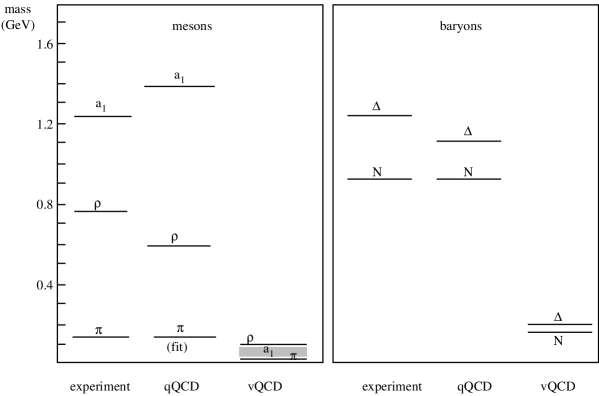
Figure 23: Spectrum of valence (vQCD) and quenched (qQCD) QCD from [274].

The main conclusion from figure 23 is that the hyperfine splittings seem to have been reduced for light hadrons.

Valence QCD still has the physics of gluon exchange, so the near degeneracy of the nucleon and $\Delta$, suggests that the “Z” graphs are the important mechanism behind the nucleon-delta mass splitting. For heavy hadrons the results from VQCD are not suppressed relative to the those from quenched QCD. For example, the VQCD prediction for the mass splitting between $B^{\star}$ and $B$ is $45.8\pm 0.4$ MeV, compared to the experimental value of 46 MeV. So the one gluon exchange is important for heavy quarks (beyond charm), but less important for light quarks. The VQCD calculations have much reduced hadron masses. For example. the nucleon mass in VQCD is reduced by 700 MeV from quenched QCD. The reduction of the vector meson mass was 537 MeV. The Kentucky group [287] attributed the reduction in hadron masses to reduction of the dynamical or constituent quark mass due to the omission of Z graphs.

Isgur [274] criticised the conclusions from the study of lattice VQCD. In particular, Isgur notes that the one boson exchange interactions, based on Z graphs, operates between two quarks, so should not effect mesons made from a quark and anti-quark. So the near degeneracy between of the $\rho$ and $\pi$ masses in figure 23 would not be expected from the suppression of Z graphs. Also Isgur [274] noted that the hadron spectrum from valence QCD was radically different from experiment (and quenched QCD). This might cause additional problems, if for example the wave-functions were very different for valence QCD compared to the real world, then this would effect the hyperfine splittings. The Kentucky group did study matrix elements that are related to the wave function of the states, but did not see any problems [288].

The current lattice calculations are currently not able to determine the correct mechanism for the mass splitting between the $\Delta$ and nucleon. Much of the lattice work has concentrated on validating one particular model, rather than also falsifying competing models. This type of physics is necessarily qualitative. For example, in the spirit of theory mutilation, ideally only one piece of physics must be removed at one time. It is not clear what effect that valence QCD has on the instanton structure of the vacuum. The modification of the Wilson fermion operator in equation 9 will also effect the zero mode structure that is of crucial importance to instanton inspired models. The operator in equation 9 does not obey

$$M^{\dagger}=\gamma_{5}M\gamma_{5}$$ (133)

for the Wilson operator $M$. There is a generalisation of equation 133 in valence QCD. There has been some work on trying to “disprove” the instanton liquid model by studying lattice QCD gauge configurations [105]. Edwards reviews the work by many groups on this [289].

Lattice QCD simulations have been used to test other assumptions made in models of the QCD dynamics. For example, there are some models of hadronic structure that are based on diquarks [290]. A critical assumption in diquark models is that two quarks actually do cluster to form a diquark. This assumption has been tested in a lattice gauge theory calculations by the Bielefeld group [291], where they found no deeply bound diquark state in Landau gauge. Leinweber [292] has claimed that lattice QCD data on the charge radii of hadrons provides evidence against scalar diquark clustering. As a test of the MIT bag model [293] and Skyrme model [294], density operators from the models were compared against results from quenched QCD.

The large $N_{c}$ limit of QCD provides much insight into QCD (see [295] for a review). Teper [296] and collaborators have studied the glueball masses in the large $N_{c}$ limit. Lattice QCD calculations can be done with any gauge group. Teper [296] et al. studied the glueball masses for $N_{c}$ = 2,3,4,5. This allowed them to estimate the size of the corrections to the $N_{c}\rightarrow\infty$ limit. As the $O(1/N_{c}^{2})$ corrections are small, it was important to control both the finite volume and lattice spacing errors.

10 WHAT LATTICE QCD IS NOT GOOD AT

In the previous sections I have implicitly assumed that all the hadrons are stable. In the real world, most hadrons are unstable to strong decays. For example the $\rho$ meson has a mass of 770 MeV and a decay width of 150 MeV. Most lattice practitioners never “worry” about the $\rho$’s decay width (in public at least). The determination of a hadron’s mass from experiment is inextricably linked to the determination of the decay width. This is perhaps most dramatically demonstrated by the problem of missing baryon resonances [297]. The quark model predicted more excited baryons [245] than were actually seen in $N\pi$ reactions. It was claimed that the additional states were not seen because they coupled very weakly to the $N\pi$ channel. The quark model did predict that the missing baryons might be seen in $N\pi\pi$ reactions [297]. There are experiments at the Jefferson lab that are trying to detect these “missing resonances” [14].

Lattice QCD calculations have to be done in Euclidean space for convergence of the path integral [35]. This implies that the amplitudes and masses from lattice calculations are real. This makes the study of resonances nontrivial, because decay widths are inherently complex quantities. This is also a problem for calculations with a finite chemical potential, although there has been some progress in this area [298].

I do not discuss the very elegant formalism of Lüscher [299] for studying unstable particles in a finite volume. The formalism and results from the scattering formalism are reviewed by Fiebig and Markum in this volume [300]. In this section, I would like to describe the possible implications for mass determinations from standard correlation functions.

The momentum is quantised on a lattice of length $L$ and periodic boundary conditions. The momentum of mesons can only take values:

$$p_{n}=\frac{2\pi n}{aL}$$ (134)

where $n$ is an integer between 0 and $L-1$. For a typical lattice, $L=16$ and $a^{-1}$ = 2.0 GeV, so the quantum of momentum is 0.79 GeV. The quantisation of momentum makes the coupling of the state to the scattering states different to that in the continuum. This “feature” has been used to advantage by Lüscher [299] in his formalism.

The quantisation of momentum has important consequences for mesons that decay via $P$ wave decays such as the $\rho$ meson. A $\rho$ meson at rest can only decay to two pions with momentum $p$ and $-p$. The decay threshold is $2\sqrt{m_{\pi}^{2}+(\frac{2\pi}{L})^{2}}$. The quantisation of momentum on the lattice does not effect the threshold for $S-$wave decays, An example of a S-wave decay is the decay of the $0^{++}$ meson to pairs of mesons. The quarks in current lattice calculations are almost light enough for the strong decay of the flavour singlet $0^{++}$ [301].

Hadron masses are extracted from lattice QCD calculations using two point correlators (equation 23). However the use of equation 23 may not be appropriate for hadrons that can decay. The most naive modification of the lattice QCD formalism caused by the introduction of decay widths is the replacement

$$m\rightarrow m+\frac{\Gamma i}{2}$$ (135)

where $\Gamma$ is the decay width. This modifies equation 23

$$c(t)=a_{0}e^{-m_{0}t}e^{-\frac{\Gamma it}{2}}+\cdots$$ (136)

that is used to extract the masses from correlators. There are a number of problems with equation 136, so a more thorough derivation is required.

I review the work by Michael [302] (see also the text book by Brown [303] ) on the effect of decays on two point functions. I will consider two scalar fields ($\sigma,\pi$) interacting with the interaction $\sigma\pi\pi$ The mass of the $\pi$ particle is $\mu$. To study the implications of particle decay on the two point correlator, consider the renormalisation of the propagator of the $\sigma$ particle in Euclidean space

$$P_{B}^{-1}(p)=p^{2}+m^{2}$$ (137)

The effect of the interaction of the $\pi$ particle with the $\sigma$ particle renormalises the $\sigma$ propagator.

$$P^{-1}(p)=p^{2}+m^{2}-X(p^{2})$$ (138)

where $X$ is the self energy.

Masses are extracted from lattice QCD calculations using the time sliced propagator:

$$G(t) = \frac{1}{2\pi}\int^{\infty}_{-\infty}dp_{0}e^{ip_{0}t}P(p_{0},\underline{0})$$ (139)

$$= \frac{1}{\pi}\int_{2\mu}^{\infty}dEe^{-Et}\rho(E)$$ (140)

where

$$\rho(E)=\frac{ImX(E)}{(m^{2}-E^{2}-X)^{2}}$$ (141)

If the pole around $E\sim-M$ is neglected then the expression for the spectral density is

$$\rho(E)=\frac{1}{2M}\frac{\gamma(E)}{(M-E)^{2}+\gamma(E)^{2}}$$ (142)

In the limit $\gamma\ll(M-2\mu),(M-2\mu)t\gg 1$

$$G(t)=\frac{1}{2M}e^{-Mt}\cos(\gamma t)+\frac{\gamma e^{-2\mu t}}{2\pi M(M-2\mu)^{2}t}$$ (143)

In figure 24, I plot separately the log of the first and second terms in equation 143 using the parameters: ($M=0.5,\gamma=0.05,\mu=0.1$). The breakdown of a pure exponential decay can be seen for the second term.

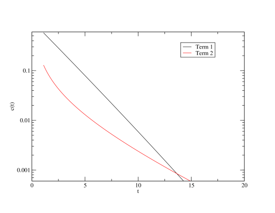
Figure 24: Resonant correlators from equation 143.

There is no evidence for the breakdown of the simple exponential fit model in current lattice calculations (apart from the effects of chiral artifacts in quenched QCD [85]). This effect may become apparent as the sea quark masses are reduced to where particle decay is energetically allowed.

The maximum entropy approach [304, 79] to extracting masses from correlators produces an estimate of the spectral density, so in principle could be used to extract the decay widths of particles. It is not clear to me whether a decay width obtained from an analysis based on maximum entropy method would be physical. Yamazaki and Ishizuka [305] have recently compared the maximum entropy approach to studying unstable particles to the method advocated by Lüscher [299] in a model theory. Yamazaki and Ishizuka claimed good agreement between the two methods.

Another way of looking for “evidence” of resonant behaviour is to look for peculiarities in the quark mass dependence of the hadron masses. One of the first applications of this idea was by DeGrand who studied the effect of $\rho$ decay on the quark mass dependence of the rho mass [154]. The mixing of the $\rho$ correlator with $\pi\pi$ states at the nonzero momentum makes the mass dependence of the $\rho$ correlator more complex than described by the theory in section 3.3. The MILC collaboration [89] have recently claimed to see some evidence for the decay of the $a_{0}$ (non-singlet $0^{++}$) meson by comparing the mass dependence of the $a_{0}$ particle in unquenched and quenched QCD.

The MILC collaboration [83] tried to look for the evidence of $\rho$ meson decay by studying the dispersion relation of the rho particle. The momentum can be injected into particle correlators, so that the hadron masses can be computed at nonzero momentum. The signal to noise gets worse, as the momentum increases, so typically the dispersion relation is only known for a few values of momentum. On the lattice the dispersion relation is of the form [306]

$$\sinh^{2}E=\sinh^{2}m+\sin^{2}p$$ (144)

The “improvement” program described in the appendix, aims to make the lattice dispersion relation closer to the continuum one. Some clever lattice theorists call this computing “the speed of light” [108].

The relationship in equation 144 predicts that the dependence of the hadron mass as a function of momentum. Consider an interpolating operator for the $\rho$ meson: $\overline{\psi}\gamma_{i}\psi$. If a unit of momentum is injected in the $z$ direction, then the $\overline{\psi}\gamma_{z}\psi$ operator will couple to the $\rho$ with one unit of moment, as well as two pions with unit momentum. The two states will mix and the masses will be modified. However, the operators: $\overline{\psi}\gamma_{y}\psi$, $\overline{\psi}\gamma_{x}\psi$ do not couple to the two pion states, essentially because $\rho\pi\pi$ interaction is zero for these kinematics. A signal for rho decay would be a different mass from the $\rho$’s polarised perpendicular and parallel to the momentum of the state. The MILC collaboration did not see this effect, perhaps because of artifacts with the type of fermions used. The UKQCD collaboration have recently claimed to see evidence for $\rho$ decay via this mechanism [307] that was consistent with the results from other methods.

In this review I have focused on just computing the masses of hadrons. The computation of decay widths from first principles is the holy grail of hadron spectroscopy. There have been very few attempts at the calculation of the decay widths from lattice QCD. The hadronic coupling constants are computed from matrix elements, rather than trying to fit expressions like equation 143 to data. Additional correlators over the standard two point correlators are required to be calculated. There have been some attempts to compute the rho to two pion coupling constant [308, 309, 310, 307]. Perhaps the most famous calculation decay widths is the calculation of partial widths for the decay of $0^{++}$ glueball were calculated by the GF11 group [311]. A clarification of the formalism for studying decay widths and mixing in lattice QCD calculations is described in [302, 69].

11 CONCLUSIONS

The computation of the light hadron mass spectrum is essential to checking the validity of lattice QCD techniques. For example, to reliably extract quark masses requires a precise and consistent calculation of the masses of the light mesons. A precise determination of the light hadron mass spectrum would unequivocally demonstrate that non-perturbative quantities can be extracted from a physically relevant quantum field theory.

The recent large scale quenched lattice QCD calculations of the spectrum of the lightest hadrons from CP-PACS [96, 196] are the benchmark for future calculations. After nearly twenty years of work the deviations of the predictions of quenched QCD from experiment have been quantified. The next generation of large scale quenched QCD calculations (if they are worth doing at all) will probably use the new fermion operators, such as overlap-Dirac operator, to push to lighter quark masses below $M_{PS}/M_{V}$ of 0.4. The light quark mass region of quenched QCD is full of pathologies, such as quenched chiral logs, that will be fun to study theoretically, but of limited or no relevance to experiment. Quenched QCD calculations will still be of some value for many interesting quantities where the uncertainty is larger than the inherent error of quenched QCD.

The main challenges in unquenched hadron spectrum calculations is determining the lattice spacing dependence and reducing the size of the quark masses used in the calculations. The unquenched calculations of the CP-PACS collaboration [134] have shown that at least three lattice spacings will be needed to obtain high “quality” results. Lattice QCD calculations with 2+1 flavours of quarks are starting to produce important results [89]. The effective field theory community is increasingly doing calculations specifically to analyse data from lattice QCD calculations.

Motivated by the “new nuclear physics” experimental programs at facilities, such as Jefferson lab [13, 14, 15], lattice calculations are starting to be used to study interesting particles such as the $N^{\star}$s. The use of more sophisticated interpolating operators and more advanced statistical techniques (such as maximum entropy techniques) may allow some information to be obtained on some of the lowest excited states of hadrons. The determination of the masses of excited states from lattice QCD would be a big step forward for hadron spectroscopy, if this was indeed possible.

The theory of hadronic physics is the ultimate postmodern playground, as it sometimes seems that the use of a particular model for hadronic physics, from a mutual incompatible set of possibilities, is almost a matter of personal preference [312]. One advantage of lattice QCD calculations is that they provide qualitative information about physical mechanisms, that is not directly accessible from experiment. If as Shuryak [276] claims, the physical picture behind the bag model and the instanton liquid model are different, then only one picture is correct, so one of them must be discarded. I hope that qualitative lattice QCD calculations can help simplify the theories behind hadronic spectroscopy by ruling out the underlying pictures behind certain classes of models. The aim of simplifying the theory of hadronic physics is a stated aim of the current experimental program [237, 272].

There are number of interesting “challenges” for hadron spectrum calculations beyond the critical task of reducing the errors in lattice QCD calculations:

• Can the resonant nature of the $\rho$ meson be determined from lattice QCD?

• Can improved lattice calculations determine the structure of the Roper resonance (first excited state of the nucleon). For over thirty five years, there have been many speculations on the nature of the Roper resonance. Can lattice QCD close this issue?

• Can the physical mechanism behind the hyperfine splittings in mesons and baryons be determined from lattice QCD?

• Can lattice QCD calculations be used to simplify hadronic physics by ruling out (or perhaps even validating) the bag model?

12 ACKNOWLEDGEMENTS

This work is supported by PPARC. I thank members of the UKQCD and MILC collaborations for discussions. I thank Chris Michael for reading the manuscript.

Appendix A TECHNICAL DETAILS

To outsiders (physicists who live in continuum), the lattice gauge theory community most seem like a very inward looking bunch. A large fraction of research in lattice gauge is on improving the methods used in lattice calculations. Improving the methods used in lattice calculations leads to smaller and more believable error bars and hence is a good thing! Currently, the biggest improvements in the methodology of lattice QCD calculations are coming from “better“ lattice representations of the continuum Dirac operator. The “new” lattice representations of the Dirac operator have either reduced lattice spacing dependence or a better chiral symmetry.

The importance of the dependence of the results on the lattice spacing has been stressed through out this review. As the results of lattice calculations are extrapolated to the continuum, the calculations would be more precise if the lattice spacing dependence of quantities was weak. The computational cost of reducing the lattice spacing used in lattice QCD calculations from equation 46 is very large, hence it is advantageous to use coarser lattice spacings [107, 313].

A standard technique from numerical analysis is to use derivatives that are closer approximations to the continuum derivatives. For example the lattice derivative in equation 146 should be more accurate with a larger lattice spacing than derivative in equation 145.

$$\frac{f(x+a)-f(x-a)}{2a}=\frac{df}{dx}+O(a^{2})$$ (145)

$$\frac{4}{3}\{\frac{f(x+a)-f(x-a)}{2a}-\frac{f(x+2a)-f(x-2a)}{16a}\}=\frac{df}{dx}+O(a^{4})$$ (146)

However in a quantum field theory there are additional complications, such as the operators in equation 146 mixing under renormalisation.

There is a formalism due to Symanzik [314, 315] called improvement where new terms are added to the lattice action that cancel $O(a)$ terms (irrelevant operators) in a way that is consistent with quantum field theory. The required terms in the improved Lagrangian can be simplified by the use of field redefinitions in the path integral [316]. A very elegant numerical procedure to improve the Wilson fermion action has been developed by the ALPHA collaboration (see the review [189] by Lüscher).

The Wilson fermion operator in equation 9 differs from the continuum Lagrangian by $O(a)$ terms. The improvement scheme used in most lattice QCD calculations with Wilson fermions is called clover improvement. The clover term [316] is added to the Wilson fermion operator in equation 9.

$$S_{f}^{clover}=S_{f}^{W}+c_{SW}\frac{ia\kappa}{2}\sum_{x}(\overline{\psi_{x}}\sigma_{\nu\mu}F_{\nu\mu}\psi_{x})$$ (147)

where $F_{\nu\mu}$ is the lattice field strength tensor.

If the $c_{SW}$ coefficient computed in perturbation theory is used then the errors in the results from the lattice calculation are $O(ag^{4})$. The ALPHA collaboration [317] have computed $c_{SW}$ to all orders in $g^{2}$ using a numerical technique. The result for $c_{SW}$ from ALPHA is

$$c_{SW}=\frac{1-0.656g^{2}-0.152g^{4}-0.054g^{6}}{1-0.922g^{2}}$$ (148)

for $0<g<1$, where $g$ is the coupling. The estimate of $c_{SW}$, by ALPHA collaboration, agrees with the one loop perturbation theory for $g<1/2$.

The clover improvement program for Wilson fermions has had many practical successes. Unfortunately, it is computationally very costly to reach light quark masses in quenched or unquenched lattice calculations that use the clover fermion operator [130]. Hence, attention has focused on also improving the eigenvalue spectrum of the lattice representation of the Dirac operator.

The design of fermion operators on the lattice has a deep connection with chiral symmetry and the global chiral anomaly. The theoretical complications with transcribing the Dirac operator to the lattice are reviewed in many places [20, 17]. Our understanding of chiral symmetry on the lattice has recently increased by the rediscovery of the Ginsparg-Wilson relation [318]

$$M\gamma_{5}+\gamma_{5}M=aM\gamma_{5}M$$ (149)

where $M$ is the fermion operator in equation 8 at zero mass. Equation 149 smoothly matches onto the chiral symmetry equation in the continuum as the lattice spacing is taken to zero. Lattice fermion operators that obey the Ginsparg-Wilson relation (equation 149) have a form of lattice chiral symmetry [319]. Explicit solutions, such as overlap-Dirac [320] or perfect actions [321], to equation 149 are known. Actions that obey the Ginsparg-Wilson relation are increasingly being used for quenched QCD calculations [322]. Domain Wall actions, that can loosely be thought of as being approximate solutions to the Ginsparg-Wilson relation, have been used in calculations [323, 324] of the matrix elements for the $\epsilon^{\prime}/\epsilon$.

The main downside of fermion operators that obey the Ginsparg-Wilson relation is that they are computationally expensive. In a review of the literature, Jansen argues [325] that overlap-Dirac type operators are roughly 100 times more expensive computationally than calculations with standard Wilson fermions. The development of new algorithms should reduce this difference in computational cost [197]. The various versions of the overlap-Dirac operator are cheap enough to use for quenched calculations. I speculate that there will be an increasing trend to use overlap-Dirac type operators for quenched calculations. It will be some time before unquenched calculations, that are useful for phenomenology, are performed with overlap-Dirac operators. Unquenched calculations of QCD with domain wall fermions have just started [326].

A more pragmatic development in the design of light fermion actions is the development of improved staggered fermion actions [90, 327]. This class of action is being used for unquenched lattice QCD calculations with very light quarks (see table 3) by the MILC collaboration. The problem with standard Kogut-Susskind quarks was that the formalism broke flavour symmetry. So numerical calculations usually had fifteen pions split by a considerable amount from the Goldstone boson pion. The new variants of fermion operators in the staggered formulations have much reduced flavour symmetry breaking. The improved staggered quark formalism is quite ugly compared to actions that are solutions of the Ginsparg-Wilson relation, but lattice QCD is a pragmatic subject and utility wins out over beauty. It is not understood why calculations using improved staggered quarks are much faster [82] than calculations using Wilson fermions [81].

References

- [1] D. Weingarten, Phys. Lett. B109, 57 (1982),
- [2] H. Hamber and G. Parisi, Phys. Rev. Lett. 47, 1792 (1981),
- [3] F. Butler, H. Chen, J. Sexton, A. Vaccarino, and D. Weingarten, Phys. Rev. Lett. 70, 2849 (1993), hep-lat/9212031,
- [4] F. Butler, H. Chen, J. Sexton, A. Vaccarino, and D. Weingarten, Nucl. Phys. B430, 179 (1994), hep-lat/9405003,
- [5] M. Beneke, (2002), hep-lat/0201011,
- [6] Particle Data Group, K. Hagiwara et al., Phys. Rev. D66, 010001 (2002),
- [7] H. Wittig, (2002), hep-lat/0210025,
- [8] C. Michael, (2003), hep-lat/0302001,
- [9] C. Michael, Phys. Scripta T99, 7 (2002), hep-lat/0111056,
- [10] C. Davies, The heavy hadron spectrum, 1997, hep-ph/9710394.
- [11] C. Davies, Lattice qcd, 2002, hep-ph/0205181.
- [12] C. McNeile, (2002), hep-lat/0210026,
- [13] CLAS, P. Rossi, (2003), hep-ex/0302032,
- [14] V. D. Burkert, (2002), hep-ph/0210321,
- [15] V. D. Burkert, (2001), hep-ph/0106143,
- [16] I. Montvay and G. Munster, Quantum fields on a lattice , Cambridge, UK: Univ. Pr. (1994) (Cambridge monographs on mathematical physics).
- [17] H. J. RotheLattice gauge theories: An Introduction Vol. 59 (, 1997),
- [18] J. Smit, Introduction to quantum fields on a lattice: A robust mate , Cambridge, UK: Univ. Pr. (2002).
- [19] M. Creutz, QUARKS, GLUONS AND LATTICES , Cambridge, Uk: Univ. Pr. ( 1983) ( Cambridge Monographs On Mathematical Physics).
- [20] R. Gupta, Introduction to lattice qcd, 1997, hep-lat/9807028.
- [21] A. S. Kronfeld, (2002), hep-lat/0205021,
- [22] C. T. H. Davies et al., (1998), hep-lat/9801024,
- [23] T. DeGrand, C. DeTar, R. Sugar, and D. Toussaint, (1998), hep-lat/9811023,
- [24] M. Mueller-Preussker et al., (2002), hep-lat/0203004,
- [25] G. S. Bali, (2003), nucl-th/0302039,
- [26] R. G. Edwards, (2002), hep-lat/0210027,
- [27] S. Gottlieb, Nucl. Phys. Proc. Suppl. 53, 155 (1997), hep-lat/9608107,
- [28] R. D. Mawhinney, Nucl. Phys. Proc. Suppl. 83, 57 (2000), hep-lat/0001032,
- [29] S. Aoki, Nucl. Phys. Proc. Suppl. 94, 3 (2001), hep-lat/0011074,
- [30] D. Toussaint, Nucl. Phys. Proc. Suppl. 106, 111 (2002), hep-lat/0110010,
- [31] T. Kaneko, (2001), hep-lat/0111005,
- [32] M. Di Pierro, (2000), hep-lat/0009001,
- [33] M. Di Pierro, (1998), hep-lat/9811036,
- [34] M. Di Pierro, (2000), hep-lat/0004007,
- [35] J. Glimm and A. Jaffe, New York, Usa: Springer ( 1987) 535p.
- [36] J. E. Mandula, G. Zweig, and J. Govaerts, Nucl. Phys. B228, 91 (1983),
- [37] J. E. Mandula and E. Shpiz, Nucl. Phys. B232, 180 (1984),
- [38] G. P. Lepage and P. B. Mackenzie, Phys. Rev. D48, 2250 (1993), hep-lat/9209022,
- [39] UKQCD, D. S. Henty and R. D. Kenway, Phys. Lett. B289, 109 (1992), hep-lat/9206009,
- [40] S. Elitzur, Phys. Rev. D12, 3978 (1975),
- [41] B. Velikson and D. Weingarten, Nucl. Phys. B249, 433 (1985),
- [42] S. Gottlieb, Presented at Conf. ’Advances in Lattice Gauge Theory’, Tallahassee, FL, Apr 10-13, 1985.
- [43] A. Duncan, E. Eichten, and H. Thacker, Phys. Lett. B303, 109 (1993),
- [44] M. W. Hecht et al., Phys. Rev. D47, 285 (1993), hep-lat/9208005,
- [45] M. W. Hecht and T. A. DeGrand, Phys. Rev. D46, 2155 (1992),
- [46] UKQCD, P. Lacock, A. McKerrell, C. Michael, I. M. Stopher, and P. W. Stephenson, Phys. Rev. D51, 6403 (1995), hep-lat/9412079,
- [47] A. Billoire, E. Marinari, and G. Parisi, Phys. Lett. B162, 160 (1985),
- [48] UKQCD, C. R. Allton et al., Phys. Rev. D47, 5128 (1993), hep-lat/9303009,
- [49] J. W. Negele and H. Orland, REDWOOD CITY, USA: ADDISON-WESLEY (1988) 459 P. (FRONTIERS IN PHYSICS, 68).
- [50] A. Duncan, S. Pernice, and J. Yoo, Phys. Rev. D65, 094509 (2002), hep-lat/0112036,
- [51] J. W. Negele, Nucl. Phys. Proc. Suppl. 73, 92 (1999), hep-lat/9810053,
- [52] UKQCD, C. McNeile, Data storage issues in lattice qcd calculations, 2000, hep-lat/0003009.
- [53] UKQCD, C. T. H. Davies, A. C. Irving, R. D. Kenway, and C. M. Maynard, (2002), hep-lat/0209121,
- [54] P. Maris and C. D. Roberts, (2003), nucl-th/0301049,
- [55] C. D. Roberts and A. G. Williams, Prog. Part. Nucl. Phys. 33, 477 (1994), hep-ph/9403224,
- [56] A. Frommer, Nucl. Phys. Proc. Suppl. 53, 120 (1997), hep-lat/9608074,
- [57] G. M. de Divitiis, R. Frezzotti, M. Masetti, and R. Petronzio, Phys. Lett. B382, 393 (1996), hep-lat/9603020,
- [58] UKQCD, C. Michael and J. Peisa, Phys. Rev. D58, 034506 (1998), hep-lat/9802015,
- [59] A. Duncan and E. Eichten, Phys. Rev. D65, 114502 (2002), hep-lat/0112028,
- [60] M. C. Chu, J. M. Grandy, S. Huang, and J. W. Negele, Phys. Rev. D48, 3340 (1993), hep-lat/9306002,
- [61] UKQCD, S. J. Hands, P. W. Stephenson, and A. McKerrell, Phys. Rev. D51, 6394 (1995), hep-lat/9412065,
- [62] T. DeGrand, Phys. Rev. D64, 094508 (2001), hep-lat/0106001,
- [63] E. V. Shuryak, Rev. Mod. Phys. 65, 1 (1993),
- [64] G. P. Lepage et al., Nucl. Phys. Proc. Suppl. 106, 12 (2002), hep-lat/0110175,
- [65] C. Michael, Phys. Rev. D49, 2616 (1994), hep-lat/9310026,
- [66] C. Michael and A. McKerrell, Phys. Rev. D51, 3745 (1995), hep-lat/9412087,
- [67] C. Michael and M. Teper, Nucl. Phys. B314, 347 (1989),
- [68] M. Luscher and U. Wolff, Nucl. Phys. B339, 222 (1990),
- [69] UKQCD, C. McNeile and C. Michael, Phys. Rev. D63, 114503 (2001), hep-lat/0010019,
- [70] T. Draper and C. McNeile, Nucl. Phys. Proc. Suppl. 34, 453 (1994), hep-lat/9401013,
- [71] G. P. Lepage, Nucl. Phys. Proc. Suppl. 26, 45 (1992),
- [72] T. A. DeGrand and M. W. Hecht, Phys. Rev. D46, 3937 (1992), hep-lat/9206011,
- [73] UKQCD, C. R. Allton et al., Phys. Rev. D65, 054502 (2002), hep-lat/0107021,
- [74] M. A. Shifman, World Sci. Lect. Notes Phys. 62, 1 (1999),
- [75] D. B. Leinweber, Phys. Rev. D51, 6369 (1995), nucl-th/9405002,
- [76] C. Allton and S. Capitani, Nucl. Phys. B526, 463 (1998), hep-lat/9712006,
- [77] C. Allton, D. Blythe, and J. Clowser, Nucl. Phys. Proc. Suppl. 109, 192 (2002), hep-lat/0202024,
- [78] A. Bochkarev and P. de Forcrand, Nucl. Phys. B477, 489 (1996), hep-lat/9505025,
- [79] CP-PACS, T. Yamazaki et al., Phys. Rev. D65, 014501 (2002), hep-lat/0105030.
- [80] Y. Nakahara, M. Asakawa, and T. Hatsuda, Phys. Rev. D60, 091503 (1999), hep-lat/9905034,
- [81] TXL, T. Lippert, Nucl. Phys. Proc. Suppl. 106, 193 (2002), hep-lat/0203009,
- [82] S. Gottlieb, Nucl. Phys. Proc. Suppl. 106, 189 (2002), hep-lat/0112039,
- [83] C. W. Bernard et al., Phys. Rev. D48, 4419 (1993), hep-lat/9305023,
- [84] J.-W. Chen, Phys. Lett. B543, 183 (2002), hep-lat/0205014,
- [85] W. Bardeen, A. Duncan, E. Eichten, N. Isgur, and H. Thacker, Phys. Rev. D65, 014509 (2002), hep-lat/0106008,
- [86] W.-J. Lee and D. Weingarten, Phys. Rev. D61, 014015 (2000), hep-lat/9910008,
- [87] P. H. Damgaard, M. C. Diamantini, P. Hernandez, and K. Jansen, Nucl. Phys. B629, 445 (2002), hep-lat/0112016,
- [88] W. Bardeen, A. Duncan, E. Eichten, G. Hockney, and H. Thacker, Phys. Rev. D57, 1633 (1998), hep-lat/9705008,
- [89] C. W. Bernard et al., Phys. Rev. D64, 054506 (2001), hep-lat/0104002,
- [90] MILC, C. W. Bernard et al., Phys. Rev. D61, 111502 (2000), hep-lat/9912018,
- [91] HPQCD, A. Gray et al., (2002).
- [92] R. Sommer, Nucl. Phys. B411, 839 (1994), hep-lat/9310022,
- [93] G. S. Bali, Phys. Rept. 343, 1 (2001), hep-ph/0001312,
- [94] M. Creutz, L. Jacobs, and C. Rebbi, Phys. Rept. 95, 201 (1983),
- [95] C. R. Allton, (1996), hep-lat/9610016,
- [96] CP-PACS, S. Aoki et al., Phys. Rev. D67, 034503 (2003), hep-lat/0206009,
- [97] C. J. Morningstar and M. J. Peardon, Phys. Rev. D60, 034509 (1999), hep-lat/9901004,
- [98] C. Morningstar and M. J. Peardon, Nucl. Phys. Proc. Suppl. 83, 887 (2000), hep-lat/9911003,
- [99] M. Guagnelli, K. Jansen, and R. Petronzio, Phys. Lett. B457, 153 (1999), hep-lat/9901016,
- [100] T. DeGrand and A. Hasenfratz, Phys. Rev. D64, 034512 (2001), hep-lat/0012021,
- [101] T. Schafer and E. V. Shuryak, Rev. Mod. Phys. 70, 323 (1998), hep-ph/9610451,
- [102] M. Teper, Nucl. Phys. Proc. Suppl. 83, 146 (2000), hep-lat/9909124,
- [103] A. Hasenfratz and C. Nieter, Phys. Lett. B439, 366 (1998), hep-lat/9806026.
- [104] A. Hasenfratz, Phys. Lett. B476, 188 (2000), hep-lat/9912053,
- [105] I. Horvath, N. Isgur, J. McCune, and H. B. Thacker, Phys. Rev. D65, 014502 (2002), hep-lat/0102003,
- [106] I. Horvath et al., Phys. Rev. D66, 034501 (2002), hep-lat/0201008,
- [107] M. G. Alford, W. Dimm, G. P. Lepage, G. Hockney, and P. B. Mackenzie, Phys. Lett. B361, 87 (1995), hep-lat/9507010,
- [108] M. G. Alford, T. R. Klassen, and G. P. Lepage, Phys. Rev. D58, 034503 (1998), hep-lat/9712005,
- [109] M. G. Alford and R. L. Jaffe, Nucl. Phys. B578, 367 (2000), hep-lat/0001023,
- [110] MILC, T. DeGrand, Phys. Rev. D58, 094503 (1998), hep-lat/9802012,
- [111] UKQCD, C. R. Allton et al., Phys. Rev. D60, 034507 (1999), hep-lat/9808016,
- [112] UKQCD, A. C. Irving et al., Phys. Rev. D58, 114504 (1998), hep-lat/9807015,
- [113] S. R. Sharpe, (1998), hep-lat/9811006,
- [114] C. Bernard et al., (2002), hep-lat/0209086,
- [115] W. Detmold, W. Melnitchouk, J. W. Negele, D. B. Renner, and A. W. Thomas, Phys. Rev. Lett. 87, 172001 (2001), hep-lat/0103006,
- [116] H. Georgi, Ann. Rev. Nucl. Part. Sci. 43, 209 (1993),
- [117] G. P. Lepage, (1997), nucl-th/9706029,
- [118] D. B. Kaplan, (1995), nucl-th/9506035,
- [119] S. Scherer, (2002), hep-ph/0210398,
- [120] S. Weinberg, Physica A96, 327 (1979),
- [121] A. Manohar and H. Georgi, Nucl. Phys. B234, 189 (1984),
- [122] J. Gasser and H. Leutwyler, Nucl. Phys. B250, 465 (1985),
- [123] C. W. Bernard and M. F. L. Golterman, Phys. Rev. D49, 486 (1994), hep-lat/9306005,
- [124] S. R. Sharpe and N. Shoresh, Phys. Rev. D62, 094503 (2000), hep-lat/0006017,
- [125] S. R. Sharpe, Phys. Rev. D56, 7052 (1997), hep-lat/9707018,
- [126] ALPHA, J. Heitger, R. Sommer, and H. Wittig, Nucl. Phys. B588, 377 (2000), hep-lat/0006026,
- [127] W. Bardeen, A. Duncan, E. Eichten, and H. Thacker, Phys. Rev. D62, 114505 (2000), hep-lat/0007010,
- [128] UKQCD, A. C. Irving, C. McNeile, C. Michael, K. J. Sharkey, and H. Wittig, Phys. Lett. B518, 243 (2001), hep-lat/0107023,
- [129] D. R. Nelson, G. T. Fleming, and G. W. Kilcup, Phys. Rev. Lett. 90, 021601 (2003), hep-lat/0112029,
- [130] UKQCD, A. C. Irving, (2002), hep-lat/0208065.
- [131] J. Bijnens, G. Ecker, and J. Gasser, (1994), hep-ph/9411232,
- [132] G. Ecker, J. Gasser, A. Pich, and E. de Rafael, Nucl. Phys. B321, 311 (1989),
- [133] D. B. Kaplan and A. V. Manohar, Phys. Rev. Lett. 56, 2004 (1986),
- [134] CP-PACS, A. Ali Khan et al., Phys. Rev. D65, 054505 (2002), hep-lat/0105015,
- [135] N. H. Fuchs, H. Sazdjian, and J. Stern, Phys. Lett. B269, 183 (1991),
- [136] M. Knecht and J. Stern, (1994), hep-ph/9411253,
- [137] L. Giusti, F. Rapuano, M. Talevi, and A. Vladikas, Nucl. Phys. B538, 249 (1999), hep-lat/9807014,
- [138] P. Hernandez, K. Jansen, and L. Lellouch, Phys. Lett. B469, 198 (1999), hep-lat/9907022,
- [139] G. Ecker, (1998), hep-ph/9805500,
- [140] T. Morozumi, A. I. Sanda, and A. Soni, Phys. Rev. D46, 2240 (1992),
- [141] A. Morel, J. Phys. (France) 48, 1111 (1987),
- [142] S. R. Sharpe, Phys. Rev. D41, 3233 (1990),
- [143] C. W. Bernard and M. F. L. Golterman, Phys. Rev. D46, 853 (1992), hep-lat/9204007,
- [144] M. Golterman, (1997), hep-ph/9710468,
- [145] G. Rupak and N. Shoresh, (2002), hep-lat/0201019,
- [146] S. R. Sharpe and J. Singleton, Robert, Phys. Rev. D58, 074501 (1998), hep-lat/9804028,
- [147] qq+q, F. Farchioni, C. Gebert, I. Montvay, E. Scholz, and L. Scorzato, Phys. Lett. B561, 102 (2003), hep-lat/0302011,
- [148] U. G. Meissner, Phys. Rept. 161, 213 (1988),
- [149] G. Ecker, J. Gasser, H. Leutwyler, A. Pich, and E. de Rafael, Phys. Lett. B223, 425 (1989),
- [150] J. Bijnens, P. Gosdzinsky, and P. Talavera, Nucl. Phys. B501, 495 (1997), hep-ph/9704212,
- [151] E. Jenkins, A. V. Manohar, and M. B. Wise, Phys. Rev. Lett. 75, 2272 (1995), hep-ph/9506356,
- [152] M. Booth, G. Chiladze, and A. F. Falk, Phys. Rev. D55, 3092 (1997), hep-ph/9610532,
- [153] C.-K. Chow and S.-J. Rey, Nucl. Phys. B528, 303 (1998), hep-ph/9708432,
- [154] T. A. DeGrand, Phys. Rev. D43, 2296 (1991),
- [155] D. B. Leinweber and T. D. Cohen, Phys. Rev. D49, 3512 (1994), hep-ph/9307261,
- [156] P. Geiger and N. Isgur, Phys. Rev. D41, 1595 (1990),
- [157] D. B. Leinweber, A. W. Thomas, K. Tsushima, and S. V. Wright, Phys. Rev. D64, 094502 (2001), hep-lat/0104013,
- [158] A. W. Thomas, (2002), hep-lat/0208023,
- [159] D. B. Leinweber, A. W. Thomas, K. Tsushima, and S. V. Wright, Phys. Rev. D61, 074502 (2000), hep-lat/9906027,
- [160] E. Jenkins and A. V. Manohar, Phys. Lett. B259, 353 (1991),
- [161] V. Bernard, N. Kaiser, J. Kambor, and U. G. Meissner, Nucl. Phys. B388, 315 (1992),
- [162] B. Borasoy and U.-G. Meissner, Annals Phys. 254, 192 (1997), hep-ph/9607432,
- [163] J. F. Donoghue, B. R. Holstein, and B. Borasoy, Phys. Rev. D59, 036002 (1999), hep-ph/9804281,
- [164] D. B. Kaplan, M. J. Savage, and M. B. Wise, Nucl. Phys. B478, 629 (1996), nucl-th/9605002,
- [165] E. Jenkins, Nucl. Phys. B368, 190 (1992),
- [166] A. W. Thomas, D. B. Leinweber, K. Tsushima, and S. V. Wright, Nucl. Phys. A663, 973 (2000), nucl-th/9909041,
- [167] U.-G. Meissner, (1998), hep-ph/9810276,
- [168] R. D. Young, D. B. Leinweber, and A. W. Thomas, (2002), hep-lat/0212031,
- [169] R. Lewis and P.-P. A. Ouimet, Phys. Rev. D64, 034005 (2001), hep-ph/0010043,
- [170] B. Borasoy, R. Lewis, and P.-P. A. Ouimet, Phys. Rev. D65, 114023 (2002), hep-ph/0203199,
- [171] T. Becher and H. Leutwyler, Eur. Phys. J. C9, 643 (1999), hep-ph/9901384,
- [172] A. R. Hoch and R. R. Horgan, Nucl. Phys. B380, 337 (1992),
- [173] C. R. Allton, V. Gimenez, L. Giusti, and F. Rapuano, Nucl. Phys. B489, 427 (1997), hep-lat/9611021,
- [174] UKQCD, P. Lacock and C. Michael, Phys. Rev. D52, 5213 (1995), hep-lat/9506009,
- [175] L. Maiani and G. Martinelli, Phys. Lett. B178, 265 (1986),
- [176] K. C. Bowler et al., Phys. Lett. B162, 354 (1985),
- [177] Ape, P. Bacilieri et al., Nucl. Phys. B317, 509 (1989),
- [178] M. Fukugita, H. Mino, M. Okawa, and A. Ukawa, Phys. Rev. Lett. 68, 761 (1992),
- [179] B. Sakita, World Sci. Lect. Notes Phys. 1, 1 (1985),
- [180] M. Luscher, Phys. Lett. B118, 391 (1982),
- [181] M. Luscher, Nucl. Phys. B219, 233 (1983),
- [182] ALPHA, J. Garden, J. Heitger, R. Sommer, and H. Wittig, Nucl. Phys. B571, 237 (2000), hep-lat/9906013,
- [183] J. Gasser and H. Leutwyler, Phys. Lett. B184, 83 (1987),
- [184] G. Colangelo, S. Durr, and R. Sommer, (2002), hep-lat/0209110,
- [185] QCDSF, A. Ali Khan et al., (2002), hep-lat/0209111,
- [186] S. Antonelli et al., Phys. Lett. B345, 49 (1995), hep-lat/9405012,
- [187] I. Montvay, Rev. Mod. Phys. 59, 263 (1987),
- [188] B. Orth et al., Nucl. Phys. Proc. Suppl. 106, 269 (2002), hep-lat/0110158,
- [189] M. Luscher, (1998), hep-lat/9802029,
- [190] J. D. Bjorken, Presented at the SLAC Summer Institute on Particle Physics, Stanford, Calif., Jul 9-20, 1979.
- [191] P. van Baal, (2000), hep-ph/0008206,
- [192] UKQCD, K. C. Bowler et al., Phys. Rev. D62, 054506 (2000), hep-lat/9910022,
- [193] F. James and M. Roos, Comput. Phys. Commun. 10, 343 (1975),
- [194] UKQCD, C. R. Allton et al., Phys. Lett. B284, 377 (1992), hep-lat/9205016,
- [195] ALPHA, M. Guagnelli, R. Sommer, and H. Wittig, Nucl. Phys. B535, 389 (1998), hep-lat/9806005,
- [196] CP-PACS, S. Aoki et al., Phys. Rev. Lett. 84, 238 (2000), hep-lat/9904012,
- [197] BGR, C. Gattringer et al., (2003), hep-lat/0307013,
- [198] M. Della Morte, R. Frezzotti, and J. Heitger, Nucl. Phys. Proc. Suppl. 106, 260 (2002), hep-lat/0110166,
- [199] M. Gockeler et al., Phys. Rev. D57, 5562 (1998), hep-lat/9707021,
- [200] UKQCD, C. McNeile and C. Michael, Nucl. Phys. Proc. Suppl. 106, 251 (2002), hep-lat/0110108,
- [201] P. Hasenfratz, S. Hauswirth, T. Jorg, F. Niedermayer, and K. Holland, (2002), hep-lat/0205010,
- [202] CP-PACS, A. Ali Khan et al., Phys. Rev. Lett. 85, 4674 (2000), hep-lat/0004010,
- [203] TXL, U. Glassner et al., Phys. Lett. B383, 98 (1996), hep-lat/9604014,
- [204] TXL, G. S. Bali et al., Phys. Rev. D62, 054503 (2000), hep-lat/0003012,
- [205] ALPHA, K. Jansen and R. Sommer, Nucl. Phys. B530, 185 (1998), hep-lat/9803017,
- [206] MILC, C. W. Bernard et al., Phys. Rev. D56, 7039 (1997), hep-lat/9707008,
- [207] V. Lubicz, Nucl. Phys. Proc. Suppl. 94, 116 (2001), hep-lat/0012003,
- [208] G. Martinelli and Y.-C. Zhang, Phys. Lett. B125, 77 (1983),
- [209] A. Hasenfratz, P. Hasenfratz, Z. Kunszt, and C. B. Lang, Phys. Lett. B117, 81 (1982),
- [210] A. Patel and R. Gupta, Phys. Lett. B131, 425 (1983),
- [211] UKQCD, P. Lacock, C. Michael, P. Boyle, and P. Rowland, Phys. Rev. D54, 6997 (1996), hep-lat/9605025,
- [212] T. DeGrand and M. Hecht, Phys. Lett. B275, 435 (1992),
- [213] H. B. Meyer and M. J. Teper, Nucl. Phys. B658, 113 (2003), hep-lat/0212026,
- [214] J. D. Weinstein and N. Isgur, Phys. Rev. D27, 588 (1983),
- [215] UKQCD, A. Hart, C. McNeile, and C. Michael, (2002), hep-lat/0209063,
- [216] RBC, S. Prelovsek and K. Orginos, (2002), hep-lat/0209132,
- [217] M. M. Brisudova, L. Burakovsky, and T. Goldman, Phys. Lett. B460, 1 (1999), hep-ph/9810296,
- [218] A. J. G. Hey and R. L. Kelly, Phys. Rept. 96, 71 (1983),
- [219] J. R. Forshaw and D. A. Ross, Cambridge, UK: Univ. Pr. (1997) 248 p. (Cambridge lecture notes in physics. 9).
- [220] A. Tang and J. W. Norbury, Phys. Rev. D62, 016006 (2000), hep-ph/0004078,
- [221] M. M. Brisudova, L. Burakovsky, and T. Goldman, Phys. Rev. D61, 054013 (2000), hep-ph/9906293,
- [222] C. W. Bernard et al., Phys. Rev. D64, 074509 (2001), hep-lat/0103012,
- [223] G. F. Chew and S. C. Frautschi, Phys. Rev. Lett. 8, 41 (1962),
- [224] A. Donnachie, eConf C010430, T05 (2001), hep-ph/0106197,
- [225] J. Hoek and J. Smit, Nucl. Phys. B263, 129 (1986),
- [226] D. B. Leinweber, Phys. Rev. D51, 6383 (1995), nucl-th/9406001,
- [227] MILC, C. W. Bernard et al., Phys. Rev. Lett. 81, 3087 (1998), hep-lat/9805004,
- [228] MILC, C. Bernard, Phys. Rev. D65, 054031 (2002), hep-lat/0111051,
- [229] S. Kim and S. Ohta, Phys. Rev. D61, 074506 (2000), hep-lat/9912001,
- [230] R. D. Mawhinney, Nucl. Phys. Proc. Suppl. 47, 557 (1996), hep-lat/9603019,
- [231] QCDSF, M. Gockeler et al., Nucl. Phys. Proc. Suppl. 83, 203 (2000), hep-lat/9909160,
- [232] JLQCD, S. Aoki et al., (2002), hep-lat/0212039,
- [233] MILC, C. W. Bernard et al., Nucl. Phys. Proc. Suppl. 73, 198 (1999), hep-lat/9810035,
- [234] N. Isgur and G. Karl, Phys. Rev. D20, 1191 (1979),
- [235] N. Isgur, Phys. Rev. D60, 054013 (1999), nucl-th/9901032,
- [236] S. Capstick and W. Roberts, (2000), nucl-th/0008028,
- [237] N. Isgur, (2000), nucl-th/0007008,
- [238] J. N. Labrenz and S. R. Sharpe, Phys. Rev. D54, 4595 (1996), hep-lat/9605034,
- [239] QCDSF, M. Gockeler et al., Phys. Lett. B532, 63 (2002), hep-lat/0106022,
- [240] S. J. Dong et al., (2003), hep-ph/0306199,
- [241] UKQCD, C. M. Maynard and D. G. Richards, (2002), hep-lat/0209165,
- [242] S. Sasaki, T. Blum, and S. Ohta, Phys. Rev. D65, 074503 (2002), hep-lat/0102010,
- [243] D. Broemmel et al., (2003), hep-ph/0307073,
- [244] Y. Nemoto, N. Nakajima, H. Matsufuru, and H. Suganuma, (2003), hep-lat/0302013,
- [245] N. Isgur and G. Karl, Phys. Rev. D19, 2653 (1979),
- [246] P. R. Page, (2002), nucl-th/0204031,
- [247] T. Barnes, (2000), nucl-th/0009011,
- [248] W. Melnitchouk et al., Phys. Rev. D67, 114506 (2003), hep-lat/0202022,
- [249] S. Sasaki, (2003), nucl-th/0305014,
- [250] M. Gockeler et al., Nucl. Phys. B487, 313 (1997), hep-lat/9605035,
- [251] S. Kim, J. B. Kogut, and M.-P. Lombardo, Phys. Rev. D65, 054015 (2002), hep-lat/0112009,
- [252] M. Burkardt, D. B. Leinweber, and X.-m. Jin, Phys. Lett. B385, 52 (1996), hep-ph/9604450,
- [253] A. Duncan, E. Eichten, and H. Thacker, Phys. Rev. Lett. 76, 3894 (1996), hep-lat/9602005,
- [254] A. Duncan, E. Eichten, and H. Thacker, Phys. Lett. B409, 387 (1997), hep-lat/9607032,
- [255] H. R. Fiebig, W. Wilcox, and R. M. Woloshyn, Nucl. Phys. B324, 47 (1989),
- [256] L. Zhou, F. X. Lee, W. Wilcox, and J. Christensen, (2002), hep-lat/0209128,
- [257] J. Christensen, F. X. Lee, W. Wilcox, and L.-m. Zhou, (2002), hep-lat/0209043,
- [258] B. R. Holstein, (2000), hep-ph/0010129,
- [259] B. E. MacGibbon et al., Phys. Rev. C52, 2097 (1995), nucl-ex/9507001,
- [260] J. Smit and J. C. Vink, Nucl. Phys. B286, 485 (1987),
- [261] M. Bander and H. R. Rubinstein, Phys. Lett. B311, 187 (1993), hep-ph/9204224,
- [262] D. Grasso and H. R. Rubinstein, Phys. Rept. 348, 163 (2001), astro-ph/0009061,
- [263] H. R. Rubinstein, S. Solomon, and T. Wittlich, Nucl. Phys. B457, 577 (1995), hep-lat/9501001,
- [264] C. W. Bernard, T. Draper, K. Olynyk, and M. Rushton, Phys. Rev. Lett. 49, 1076 (1982),
- [265] G. Martinelli, G. Parisi, R. Petronzio, and F. Rapuano, Phys. Lett. B116, 434 (1982),
- [266] T. Draper, R. M. Woloshyn, W. Wilcox, and K.-F. Liu, Nucl. Phys. B318, 319 (1989),
- [267] T. Draper, R. M. Woloshyn, and K.-F. Liu, Phys. Lett. B234, 121 (1990),
- [268] V. Gadiyak, X.-d. Ji, and C.-w. Jung, Phys. Rev. D65, 094510 (2002), hep-lat/0112040,
- [269] S. Aoki and A. Gocksch, Phys. Rev. Lett. 63, 1125 (1989),
- [270] S. Aoki, A. Gocksch, A. V. Manohar, and S. R. Sharpe, Phys. Rev. Lett. 65, 1092 (1990),
- [271] D. Guadagnoli, V. Lubicz, G. Martinelli, and S. Simula, JHEP 04, 019 (2003), hep-lat/0210044,
- [272] S. Capstick et al., Key issues in hadronic physics, 2000, hep-ph/0012238.
- [273] N. Yamada, (2002), hep-lat/0210035,
- [274] N. Isgur, Phys. Rev. D61, 118501 (2000), hep-lat/9908009,
- [275] N. Isgur and H. B. Thacker, Phys. Rev. D64, 094507 (2001), hep-lat/0005006,
- [276] E. V. Shuryak, Lect. Notes Phys. 583, 251 (2002), hep-ph/0104249,
- [277] A. W. Thomas and W. Weise, Berlin, Germany: Wiley-VCH (2001) 389 p.
- [278] J. Greensite, (2003), hep-lat/0301023,
- [279] R. D. Loft and T. A. DeGrand, Phys. Rev. D39, 2678 (1989),
- [280] Y. Iwasaki and T. Yoshie, Phys. Lett. B216, 387 (1989),
- [281] S. Ono, Phys. Rev. D17, 888 (1978),
- [282] M. C. Chu, J. M. Grandy, S. Huang, and J. W. Negele, Phys. Rev. D49, 6039 (1994), hep-lat/9312071,
- [283] T. G. Kovacs, Phys. Rev. D62, 034502 (2000), hep-lat/9912021,
- [284] E. V. Shuryak and J. L. Rosner, Phys. Lett. B218, 72 (1989),
- [285] L. Y. Glozman, Nucl. Phys. A663, 103 (2000), hep-ph/9908423,
- [286] N. Isgur, Phys. Rev. D62, 054026 (2000), nucl-th/9908028,
- [287] K. F. Liu et al., Phys. Rev. D59, 112001 (1999), hep-ph/9806491,
- [288] K. F. Liu et al., Phys. Rev. D61, 118502 (2000), hep-lat/9912049,
- [289] R. G. Edwards, Nucl. Phys. Proc. Suppl. 106, 38 (2002), hep-lat/0111009,
- [290] M. Anselmino, E. Predazzi, S. Ekelin, S. Fredriksson, and D. B. Lichtenberg, Rev. Mod. Phys. 65, 1199 (1993),
- [291] M. Hess, F. Karsch, E. Laermann, and I. Wetzorke, Phys. Rev. D58, 111502 (1998), hep-lat/9804023,
- [292] D. B. Leinweber, Phys. Rev. D47, 5096 (1993), hep-ph/9302266,
- [293] M. Lissia, M. C. Chu, J. W. Negele, and J. M. Grandy, Nucl. Phys. A555, 272 (1993),
- [294] M. C. Chu, M. Lissia, and J. W. Negele, Nucl. Phys. A570, 521 (1994), hep-lat/9308012,
- [295] J. F. Donoghue, E. Golowich, and B. R. Holstein, Cambridge Monogr. Part. Phys. Nucl. Phys. Cosmol. 2, 1 (1992),
- [296] B. Lucini and M. Teper, JHEP 06, 050 (2001), hep-lat/0103027,
- [297] R. Koniuk and N. Isgur, Phys. Rev. Lett. 44, 845 (1980),
- [298] J. B. Kogut, (2002), hep-lat/0208077,
- [299] M. Luscher, Nucl. Phys. B364, 237 (1991),
- [300] H. R. Fiebig and H. Markum, (2002), hep-lat/0212037,
- [301] UKQCD, A. Hart and M. Teper, Phys. Rev. D65, 034502 (2002), hep-lat/0108022,
- [302] C. Michael, Nucl. Phys. B327, 515 (1989),
- [303] L. S. Brown, Quantum field theory , Cambridge, UK: Univ. Pr. (1992).
- [304] M. Asakawa, T. Hatsuda, and Y. Nakahara, Prog. Part. Nucl. Phys. 46, 459 (2001), hep-lat/0011040,
- [305] T. Yamazaki and N. Ishizuka, Phys. Rev. D67, 077503 (2003), hep-lat/0210022,
- [306] T. Bhattacharya, R. Gupta, G. Kilcup, and S. R. Sharpe, Phys. Rev. D53, 6486 (1996), hep-lat/9512021,
- [307] UKQCD, C. McNeile and C. Michael, Phys. Lett. B556, 177 (2003), hep-lat/0212020,
- [308] S. Gottlieb, P. B. Mackenzie, H. B. Thacker, and D. Weingarten, Phys. Lett. B134, 346 (1984),
- [309] R. L. Altmeyer et al., Z. Phys. C68, 443 (1995), hep-lat/9504003,
- [310] R. D. Loft and T. A. DeGrand, Phys. Rev. D39, 2692 (1989),
- [311] J. Sexton, A. Vaccarino, and D. Weingarten, Phys. Rev. Lett. 75, 4563 (1995), hep-lat/9510022,
- [312] A. Pickering, CONSTRUCTING QUARKS. A SOCIOLOGICAL HISTORY OF PARTICLE PHYSICS , Edinburgh, Uk: Univ. Pr. ( 1984).
- [313] P. Lepage, Nucl. Phys. Proc. Suppl. 60A, 267 (1998), hep-lat/9707026,
- [314] K. Symanzik, Nucl. Phys. B226, 187 (1983),
- [315] K. Symanzik, Nucl. Phys. B226, 205 (1983),
- [316] B. Sheikholeslami and R. Wohlert, Nucl. Phys. B259, 572 (1985),
- [317] M. Luscher, S. Sint, R. Sommer, P. Weisz, and U. Wolff, Nucl. Phys. B491, 323 (1997), hep-lat/9609035,
- [318] P. H. Ginsparg and K. G. Wilson, Phys. Rev. D25, 2649 (1982),
- [319] M. Luscher, Phys. Lett. B428, 342 (1998), hep-lat/9802011,
- [320] H. Neuberger, Ann. Rev. Nucl. Part. Sci. 51, 23 (2001), hep-lat/0101006,
- [321] P. Hasenfratz, Nucl. Phys. B525, 401 (1998), hep-lat/9802007,
- [322] P. Hernandez, Nucl. Phys. Proc. Suppl. 106, 80 (2002), hep-lat/0110218,
- [323] CP-PACS, J. I. Noaki et al., (2001), hep-lat/0108013,
- [324] RBC, T. Blum et al., (2001), hep-lat/0110075,
- [325] K. Jansen, Nucl. Phys. Proc. Suppl. 106, 191 (2002), hep-lat/0111062,
- [326] RBC, T. Izubuchi, (2002), hep-lat/0210011,
- [327] MILC, K. Orginos and D. Toussaint, Phys. Rev. D59, 014501 (1999), hep-lat/9805009,