Abstract

This is the first part of a study of the quark propagator and the vertex function of the vector current on the lattice in the Landau gauge and using both Wilson-clover and overlap actions. In order to be able to identify lattice artifacts and to reach large momenta we use a range of lattice spacings. The lattice artifacts turn out to be exceedingly large in this study. We present a new and very efficient method to eliminate the hypercubic (anisotropy) artifacts based on a systematic expansion on hypercubic invariants which are not $SO(4)$ invariant. A simpler version of this method has been used in previous works. This method is shown to be significantly more efficient than the popular “democratic” methods. It can of course be applied to the lattice simulations of many other physical quantities. The analysis indicates a hierarchy in the size of hypercubic artifacts: overlap larger than clover and propagator larger than vertex function. This pleads for the combined study of propagators and vertex functions via Ward identities.

PACS: 12.38.Gc (Lattice QCD calculations)

1 Introduction

The study of the quark propagator and vertex functions has been extensively pursued in the literature starting in the 70’s [1]. Lattice QCD has more recently treated this issue [2]. A systematic treatment varying the quark actions has been followed by the CSSM collaboration [3]. The scalar part of the quark propagator is related via Ward identities to the pseudoscalar vertex function. The role of the Goldstone boson pole in the latter has been thoroughly discussed [4].

Leaving aside the latter issue, we will mainly concentrate on the vector part of the quark propagator, the one which is proportional to $p\!\!\!/$. One of our main goals is to check the effect of the $A^{2}$ condensate which has been discovered via power corrections at large momenta to the gluon propagator and three point Green functions [5]-[8]. The values plotted in literature for $Z_{\psi}(p^{2})$ are extremely flat above 2 GeV [9]. At first sight this is a satisfactory feature since the perturbative-QCD corrections are known to be small. However a closer scrutiny makes it worrying since both the perturbative QCD corrections and the $A^{2}$ condensate predict a decrease which seems not to be seen. This leads us to start a very systematic study of the problem, with the following series of improvements on earlier works:

• We reach an energy of 10 GeV by matching several lattice spacings so we are in a better position to eliminate lattice artifacts.

• We make a systematic use of Ward identities relating the quark propagator and the vertex function via the constant $Z_{V}$ and study both quantities in parallel.

• We make use of a very efficient way of eliminating hypercubic artifacts. A simpler version of it was elaborated while studying gluon propagators [6], [7]. In this work we have encountered the necessity to improve significantly this method.

This last point will be the main subject of this paper. Indeed, the raw data show a shape somewhat reminiscent of a half-fishbone (fig. 1), utterly different from a smooth curve expected in the continuum. As we shall see the method elaborated in [6], [7] proves not to be powerful enough. We therefore wish to attract attention on the generalisation of the above-mentioned method which we believe is strikingly efficient and should become a very useful tool for the lattice community.

The remaining part of the work, i.e. the correction of $SO(4)$ symmetric artifacts and the resulting physics results will be presented in a later publication.

In section 2 we will recall some theoretical premises, in section 3 we will indicate the lattice simulations which we have performed, in section 4 we will describe our method to eliminate lattice artifacts and compare it to earlier methods.

2 Theoretical premisses

We work in the Landau gauge. Let us first fix the notations that we will use. We will use all along the Euclidean metric. The continuum quark propagator is a $12\times 12$ matrix $S(p_{\mu})$. The inverse propagator is expanded

$$\widetilde{S}^{-1}(p)=\delta_{a,b}Z_{\psi}(p^{2})\left(i\,p\!\!\!/+m(p^{2})\right)$$ (1)

where $a,b$ are the color indices.

Let us consider a colorless vector current $\bar{q}\gamma_{\mu}q$. The three point Green function $G_{\mu}$ is defined by

$$G_{\mu}(p,q)=\int d^{4}xd^{4}ye^{ip\cdot y-i(p+q)\cdot x}<q(y)\bar{q}(0)\gamma_{\mu}q(0)\bar{q}(x)>\ .$$ (2)

In all this paper we will restrict ourselves to the case where the vector current carries a vanishing momentum transfer $q_{\mu}$. The vertex function is then defined by

$$\Gamma_{\mu}(p,q=0)=\widetilde{S}^{-1}(p)\,G_{\mu}(p,q=0)\,\widetilde{S}^{-1}(p)\ .$$ (3)

In the following we will omit to write $q_{\mu}=0$ and we will understand $\Gamma_{\mu}(p)$ as the bare vertex function computed on the lattice. The renormalised vertex function is $Z_{V}\Gamma_{\mu}(p)$.

From Lorentz covariance and discrete symmetries

$$\Gamma_{\mu}(p)=\delta_{a,b}\left[g_{1}(p^{2})\gamma_{\mu}+ig_{2}(p^{2})p_{\mu}+g_{3}(p^{2})p_{\mu}p\!\!\!/+ig_{4}(p^{2})[\gamma_{\mu},p\!\!\!/]\right]\ .$$ (4)

The Ward identity tells us that

$$Z_{V}\Gamma_{\mu}(p)=-i\,\frac{\partial}{\partial p^{\mu}}\widetilde{S}^{-1}(p),\quad$$ (5)

which from (1)-(4) implies

$$Z_{\psi}(p^{2})=Z_{V}g_{1}(p^{2}),\quad 2\,\frac{\partial}{\partial p^{2}}Z_{\psi}(p^{2})=Z_{V}g_{3}(p^{2}),$$

$$2\,\frac{\partial}{\partial p^{2}}b(p^{2})=-Z_{V}g_{2}(p^{2}),\quad g_{4}(p^{2})=0.$$ (6)

For a conserved current, $Z_{V}=1$. We keep $Z_{V}$ since the local vector current on the lattice is not conserved; it will differ from 1 by lattice perturbative corrections which are a finite series in the “boosted” bare coupling constant, independent of $p^{2}$. However, lattice artifacts do generate a sometimes significant $p^{2}$ dependence of $Z_{V}$ at the level of raw lattice data, see for example fig. 3. We will therefore sometimes use a p-dependent raw $Z_{V}$ written $Z_{V}(p^{2})$ and defined in eq. (17)

The renormalisation scheme that we use is the one called MOM’, eq (26) in ref. [10]. The bare propagator $S(p)$ is multiplied by the renormalisation constant

$$\widetilde{S}_{\rm R}(p)=Z_{\psi}(\mu)\widetilde{S}(p),\quad{\rm whence}\quad\widetilde{S}_{\rm R}^{-1}(p)|_{p^{2}=\mu^{2}}=\delta_{a,b}\left(i\,p\!\!\!/+m(p^{2})\right)$$ (7)

This defines the quark field renormalisation. Due to the Ward identity, the factor $Z_{\psi}(\mu)^{-1}$ multiplies the bare vertex function $g_{1}$, so that $g_{1}^{\rm R}(p^{2}=\mu^{2})=Z_{V}^{-1}$.

From the anomalous dimensions computed in ref. [10] we may express the perturbative running of $Z_{\psi}$ for example as a function of the running $\alpha_{\overline{\rm MOM}}(p)$. As $Z_{V}$ in the continuum is a constant, $Z_{\psi}(p)$ and $g_{1}(p)$ have the same perturbative scale dependence.

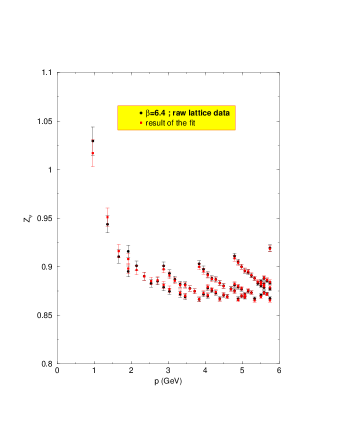
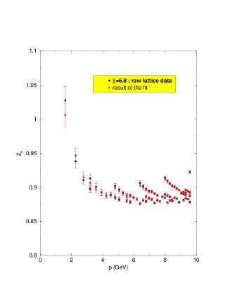
Figure 1: Fit of the raw lattice data for clover-$Z_{\psi}$ with formula (22) for $\beta=6.4$ and 6.8. For $Q(p^{2},0,0)$ we have taken a polynomial of degree eight in $p^{2}$. The fit has been done independently for each $\beta$. The raw data are represented by black circles while the fit is shown by red squares. The agreement is often such that the raw data and fit points are indistinguishable on the plot.

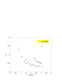
Figure 2: Raw lattice data for overlap-$Z_{\psi}$ for $\beta=6.0$ and 6.8.

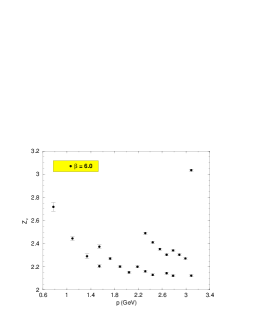
Figure 3: Raw lattice data for overlap-$Z_{V}$ for $\beta=6.0$ and 6.8.

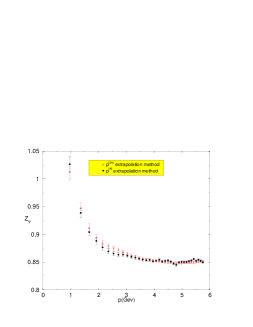
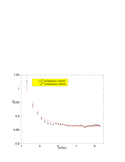
Figure 4: comparison of the “$\mathbf{p}^{[4]}$ extrapolation method, represented by black circles, with the “ $\mathbf{p}^{[2n]}$ extrapolation method ” represented by “x” symbols. The left (right) plot shows the result for clover-$Z_{\psi}$ at $\beta=6.4$ ($\beta=6.8$)

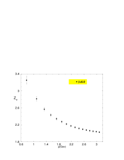
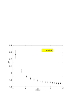
Figure 5: Lattice data for overlap-$Z_{\psi}$ after application of the “ $\mathbf{p}^{[2n]}$ extrapolation method ” for $\beta=6.0$ and 6.8.

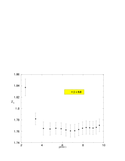
Figure 6: Lattice data for overlap-$Z_{V}$ after application of the “ $\mathbf{p}^{[2n]}$ extrapolation method ” for $\beta=6.0$ and 6.8.

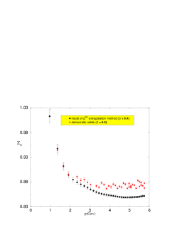
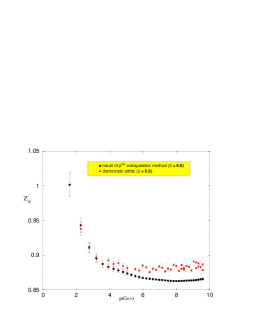
Figure 7: Red squares represent the “democratic” orbits, defined by $p^{[4]}/(p^{2})^{2}\leq.5$, for clover-$Z_{\psi}$ at $\beta=6.4,6.8$. The black circles represent the result of the $p^{[2n]}$ extrapolation method. The latter exhibit a much smoother behavior.

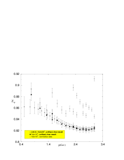
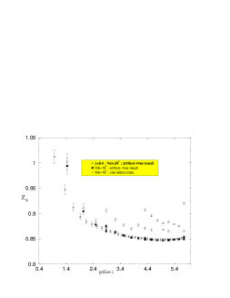
Figure 8: The white squares show the raw lattice results for clover-$Z_{\psi}$ with a volume of $16^{4}$. The black squares are the same after the artifacts computed with a volume of $24^{4}$ have been subtracted and the crosses represent the artifact-free result computed with a volume of $24^{4}$. The agreement between black squares and crosses is striking except for the smallest momentum on $16^{4}$. The figure to the left (right) is for $\beta=6.0$ ($\beta=6.4$).

3 Lattice calculations

We have used improved Wilson quarks (often called clover) with the CSW coefficients computed in [11]. 100 gauge configurations have been computed at $\beta=6.0,6.4,6.6,6.8$ with volumes $24^{4}$, $16^{4}$ and $8^{4}$. We have performed the calculation for five quark masses but in practice, for what is our concern in this paper, the quark mass dependence has non surprisingly proven to be negligible and for simplicity we will only present the results for the lightest quark mass, about 50 MeV, i.e.

$$\kappa=0.1346,\,\,0.13538,\,\,0.13515,\,\,0.13489\quad{\rm for}\quad\beta=6.0,\,\,6.4,\,\,6.6,\,\,6.8$$ (8)

It should also be mentioned that all the results presented refer to the $24^{4}$ lattices unless stated otherwise.

We have also used overlap fermions [12, 13] with about the same mass i.e.

$$a\,m_{0}=0.03,\,\,0.01667,\,\,0.01.\,\quad{\rm for}\quad\beta=6.0,\,\,6.4,\,\,6.8$$ (9)

with $s=0$ and volumes of only $16^{4}$ due to memory limitations. The bare mass $m_{0}$ and $s$ are defined from

$$D_{\rm over}=(1+s+am_{0}/2)+(1+s-am_{0}/2)\frac{D_{\rm w}(-(1+s))}{\sqrt{D_{\rm w}(-(1+s))^{\dagger}\,D_{\rm w}(-(1+s))}}$$ (10)

where $D_{\rm w}(-(1+s))$ is the Wilson-Dirac operator with a (negative) mass term $-1-s$

$$D_{\rm w}(-1-s)\equiv\frac{1}{2}\gamma_{\mu}(\nabla_{\mu}+\nabla^{*}_{\mu})-\frac{1}{2}a\nabla^{*}_{\mu}\nabla_{\mu}-1-s\,,$$ (11)

The propagators $S(x,0)$ from the origin to point $x$ have been computed and their Fourier transform

$$\widetilde{S}(p)=\sum_{x}e^{-ip\cdot x}S(x,0)$$ (12)

have been averaged among all configurations and all momenta $p_{\mu}$ within one orbit of the hypercubic symmetry group of the lattice, exactly as for gluon Green functions in [6]-[8]. In the case of overlap quarks the propagator is improved according to a standard procedure [13] which eliminates $O(a)$ discretization errors:

$$\widetilde{S}_{\ast}(p)=\frac{\widetilde{S}(p)-\frac{1}{2}}{1-am_{0}/2}$$ (13)

From now on, the notation $S(p)$ will represent the improved quark propagator in the case of overlap quarks and the standard one in the case of clover quarks.

In both cases we fit the inverse quark propagator by

$$\widetilde{S}^{-1}(p)=\delta_{a,b}\,{Z_{\psi}(p^{2})}\,\left(i\,\bar{p}\!\!\!/+m(p^{2})\right)$$ (14)

according to eq. (1) and where $\bar{p}_{\mu}$ is defined in eq. (18). The three point Green functions with vanishing momentum transfer are computed by averaging analogously over the thermalised configurations and the points in each orbit

$$G_{\mu}(p,q=0)=<\gamma_{5}\,\widetilde{S}(p)^{\dagger}\,\gamma_{5}\,\gamma_{\mu}\,\widetilde{S}(p)>.$$ (15)

where the identity $S(0,x)=\gamma_{5}S^{\dagger}(x,0)\gamma_{5}$ has been used. The vertex function is then computed according to eq. (3) and we choose for the lattice form factor $g_{1}$ :

$$g_{1}(p^{2})=\frac{1}{36}{\rm Tr}\left[\Gamma_{\mu}(p,q=0)\left(\gamma_{\mu}-\bar{p}_{\mu}\frac{\bar{p}\!\!\!/}{\bar{p}^{2}}\right)\right]$$ (16)

where the trace is understood over both color and Dirac indices.

Finally, according to the Ward identity (2) we compute $Z_{V}$ simply from

$$Z_{V}(p^{2})\equiv\frac{Z_{\psi}(p^{2})}{g_{1}(p^{2})}.$$ (17)

where the $p^{2}$-dependence of $Z_{V}$ coming from lattice artifacts has been explicitly written.

In whole this paper we will use the values in the following table 1 for the lattice spacings, which follow the $\beta$ dependence found in ref. [15],

$\beta$	6.0	6.4	6.6	6.8
$a^{-1}$ (GeV)	1.966	3.66	4.744	6.1
$a$ (fm)	0.101	0.055	0.042	0.033

Table 1: Lattices spacings

4 Elimination of lattice hypercubic artifacts

The question of eliminating lattice artifacts has been our main difficulty in the accurate study of the quark propagator. We became convinced that it was absolutely impossible to say anything sensible without an extremely careful elimination of artifacts. Here we mean mainly the ultraviolet artifacts, the infrared artifacts having never been really troublesome in this problem.

We have elaborated a very powerful method to deal with hypercubic artifacts i.e. with those ultraviolet artifacts which come from the difference between the hypercubic geometry of the lattice and the fully hyper-spherically symmetric one of the continuum Euclidean space. The principle of this method is based on identifying the artifacts which are invariant for the $H_{4}$ symmetry of the hypercube, but not for the $SO(4)$ symmetry of the continuum.

Once these artifacts have been eliminated it is obvious, as we shall show, that other - $SO(4)$-invariant ultraviolet artifacts - are present. And these turn out to be even trickier to deal with, mainly because we did not fully understand their rationale.

Therefore, we intend to restrict ourselves in this paper to a careful explanation of the hypercubic artifacts elimination method since we believe it represents a real progress and it can be useful for many other lattice calculations. The treatment of the $SO(4)$-invariant artifacts and of the physical results concerning the quark propagator will be given in a later publication.

4.1 $\mathbf{p}^{[2n]}$ extrapolation method

Since we use hypercubic lattices our results are invariant for a discrete symmetry group, $H_{4}$, a subgroup of the continuum Euclidean $SO(4)$. This implies that lattice data for momenta which are not related by an $H_{4}$ transformation but are by a $SO(4)$ rotation will in principle differ. Of course this difference must vanish when $a\to 0$ but it must be considered among the discretisation effects, i.e. ultraviolet artifacts. For example, in perturbative lattice calculations one encounters the expressions

$$\tilde{p}_{\mu}\equiv\frac{2}{a}\sin\left(\frac{ap_{\mu}}{2}\right),\quad\bar{p}_{\mu}\equiv\frac{1}{a}\sin\left(ap_{\mu}\right).$$ (18)

Both are equal to $p_{\mu}$ up to lattice artifacts:

$$\tilde{p^{2}}\equiv\sum_{\mu=1,4}\tilde{p}_{\mu}^{2}=p^{2}-\frac{1}{12}a^{2}p^{[4]}+\cdots\quad\bar{p}^{2}=p^{2}-\frac{1}{3}a^{2}p^{[4]}+\cdots\,,\,{\rm where}\,p^{[2n]}\equiv\sum_{\mu=1,4}p_{\mu}^{2n}\,.$$ (19)

All terms in the dots are proportional to $a^{2n}p^{[2n+2]}$ . $p^{2}$, $\tilde{p}^{2}$, $\bar{p}^{2}$, $a^{2}p^{[4]}$ are invariant under $H_{4}$ but only $p^{2}$ is under $SO(4)$. For example the momenta $2\pi(1,1,1,1)\,/L$ and $2\pi(2,0,0,0)\,/L$ have the same $p^{2}$ but different $p^{[4]},\tilde{p}^{2}$ and $\bar{p}^{2}$. In other words, if we call an orbit the set of momenta related by $H_{4}$ transformations, different orbits, corresponding to the same $p^{2}$, will in general have different $p^{[4]}$. The hypercubic artifacts can be detected by looking carefully for a given quantity at a given $p^{2}$ how it depends on the orbit.

One method proposed with success for the gluon propagator [7], [8] analyses a generic lattice measured quantity $Q$ as a function $Q(p^{2},p^{[4]})$. For a given value of $p^{2}$, if enough different values of $p^{[4]}$ exist the quantity $Q$ is fitted by

$$Q(p^{2},p^{[4]})=Q(p^{2},0)+\frac{\partial Q(p^{2},y)}{\partial y}|_{y=0}\,\,{p^{[4]}}.$$ (20)

where $Q(p^{2},0)$ is free of hypercubic artifacts and where $\frac{\partial Q(p^{2},y)}{\partial y}|_{y=0}$ is computed numerically for each $p^{2}$ from the slope of the lattice data for $Q(p^{2},p^{[4]})$ as a function of $p^{[4]}$. Of course, we could also consider $p^{[6]}$, etc. but usually there are not enough different orbits for one given $p^{2}$ to fit more than the $p^{[4]}$ correction.

Let us call this method the “$\mathbf{p}^{[4]}$ extrapolation method”. For the gluon propagator this method has been shown [8] to lead to a resulting function $G(p^{2},p^{[4]}=0)$ much smoother than the direct lattice results $Q(p^{2},p^{[4]})$, even if the latter are restricted, as often done, to the “democratic” momenta, i.e. to those which have the smallest $p^{[4]}$. This method could be applied with some success to the function clover-$g_{1}$ (i.e. $g_{1}$ obtained from improved Wilson quarks).

But in general, as we shall see, when applied to clover-$Z_{\psi}$ or to the quantities computed from overlap quarks, the “$\mathbf{p}^{[4]}$ extrapolation” method fails. The signal of this failure is that the resulting function $Q(p^{2},p^{[4]}=0)$ still shows sizable oscillations typical of hypercubic artifacts.

We then propose a “$\mathbf{p^{[2n]}}$ extrapolation method” which allows to eliminate much more efficiently these hypercubic artifacts. The improvement goes in two directions:

i) Instead of fitting the $p^{[4]}$ slope separately for each value of $p^{2}$ we try a global fit of the hypercubic artifacts over all values of $p^{2}$

ii) We chase hypercubic artifacts up to order $a^{4}$.

In order to perform a global fit we start from the remark that in this paper we are dealing with dimensionless quantities, $g_{1}$ and $Z_{\psi}$. It is thus natural to expect that hypercubic artifacts contribute via dimensionless quantities times a constant . Next we assume that there is a regular continuum limit which implies that in the denominator we can have only physical quantities, namely  a function of $p^{2}$. These two priors lead us to a Taylor expansion with terms of the type

$$\left(\frac{a^{2k}p^{[2k+2n]}}{(p^{2})^{n}}\right)^{m}\qquad k>0,\quad n\geq 0\quad k+n>1,\quad m>0.$$ (21)

This still leaves us with far too many terms to make sensible fits. It is reasonable to truncate this series in $a$ and we choose to expand it up to $a^{4}$. We will also truncate it to $n\leq 1$, and now comes an heuristic argument to justify this truncation.

The lattice results are $H_{4}$ invariant and thus typically functions of $\tilde{p}^{2}$, $\bar{p}^{2}$ and $\tilde{p}\cdot\bar{p}$. Dimensionless quantities will depend on ratios of these quantities and on terms  like $a^{2}\tilde{p}^{2}$. An examination of these shows that they produce anisotropic terms corresponding to $n=0$ and $n=1$ in the classification of eq. (21). For example, $a^{2}\tilde{p}^{2}$ produces from the expansion eq. (19) a term $\propto a^{4}p^{[4]}$ while $\tilde{p}\cdot\bar{p}/\bar{p}^{2}$ produces terms $\propto a^{2}p^{[4]}/p^{2}$ etc. This is also what is found in the free case [13].

Hence we fit the data according to

$$Q(p^{2},a^{2}p^{[4]},a^{4}p^{[6]},\cdots)=Q(p^{2},0,0)+c_{1}\,\frac{a^{2}p^{[4]}}{p^{2}}+c_{2}\,\left(\frac{a^{2}p^{[4]}}{p^{2}}\right)^{2}+c_{3}\,\frac{a^{4}p^{[6]}}{p^{2}}+c_{4}\,a^{4}p^{[4]}.$$ (22)

A remark is needed about the $a$ dependence of the coefficients $c_{i}$. Being dimensionless it is expected in perturbation theory that these coefficients depend only logarithmically on $a$ and taking them as constants would seem reasonable. This conjecture does not work as shown in fig. 9 which is the sign of non-perturbative ${\cal O}(a\Lambda_{\rm QCD})$ contributions. Still this figure shows a rather convincing linear dependence of the $c_{i}$’s for $Z_{\psi}$ which tells that a good global fit can be performed by expanding the coefficients: $c_{i}(a)=c_{i}^{0}+ac_{i}^{1}$. For $g_{1}$ the $a$ dependence is not linear while the hypercubic artifacts are one order of magnitude smaller.

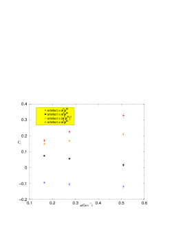
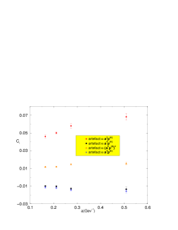
Figure 9: Coefficients of the hypercubic artifacts for $Z_{\psi}$ from overlap quarks (left) and clover (right) as a function of $a$ for $\beta=6.0,6.4,6.8$ and 6.6 in the clover case. The squares corresponds to $c_{1}$, the coefficient of $a^{2}p^{[4]}/p^{2}$, the triangles to $c_{2}$, the coefficient of $(a^{2}p^{[4]}/p^{2})^{2}$, the stars to $c_{3}$, the coefficient of $(a^{4}p^{[6]}/p^{2})^{2}$ and the circles to $c_{4}$, the coefficient of $a^{4}p^{[4]}$. It suggests a linear dependence on a, especially for the overlap quarks. The overlap artifacts are larger than the clover ones by one order of magnitude.

The functional form used for $Q(p^{2},0,0)$ does not influence significantly the resulting artifact coefficients. We can even avoid using any assumption about this functional form by taking all the values for $Q(p^{2},0,0)$ as parameters which can be fitted .

This improved correction of hypercubic artifacts turned out to be particularly necessary for $Z_{\psi}$. In fig. 1 the very strong hypercubic artifacts produce an impressive branched structure with a kind of periodicity. In fig. 4 we show the effect of both the use of eqs. (20) and (22). It turns out to that “$\mathbf{p}^{[4]}$ extrapolation method”, eq. (20), makes the branches disappear and the curve look much smoother. However it still contains some oscillations reminiscent of the hypercubic artifacts. The “$\mathbf{p}^{[2n]}$ extrapolation method”, eq. (22), brings in a further dramatic smoothing.

The same is true for overlap-computed quantities. In figs. 2 and 3 the raw lattice data for $Z_{\psi}$ and $Z_{V}$ exhibit dramatically the “half-fishbone” structure which is a symptom of strong hypercubic artifacts. In figs. 5 and 6 the same data are shown after applying the $\mathbf{p}^{[2n]}$ extrapolation method. Clearly the curves are now perfectly smooth. We will return later to the fact that $Z_{V}$ is not a constant.

Altogether we would like to stress the following hierarchy: First, the hypercubic artifacts are one order of magnitude larger for overlap quarks than for clover ones, see fig. 9. Second, for both types of quarks the hypercubic artifacts for $Z_{\psi}$ are one order of magnitude larger than those for $g_{1}$.

4.2 Comparison with the “democratic” method

The hypercubic artifacts, sometimes called “anisotropy artifacts” have been a long standing problem in lattice calculations. Studying the gluon propagator the authors of ref. [14] where aware that the problem was related to the fact that for a given momentum $p^{2}$ these artifacts were minimised when the components were as small as possible, i.e. such that the components are not too hierarchical, and that the ideal situation was the diagonal $p\propto(1,1,1,1)$, whence the name commonly used of a “democratic” repartition of the momentum in all directions. Therefore they have proposed a selection keeping only the orbits having a point within a cylinder around the diagonal. Several other criteria have been used.

In this subsection we want to compare this method of eliminating the non-democratic points to the “ $\mathbf{a}^{2}p^{[2n]}$ extrapolation method”, eq. (22). If we try to select, [14], the orbits which are in a cylinder around the diagonal with a radius $2\pi/L$, we are left with only 11 orbits among 69.

In order to have a less restrictive criterion and to make the bridge with the method used here we will use the $p^{[2n]}$’s defined in eq. (19). In our language, democracy can be translated as a small enough ratio $p^{[4]}/(p^{2})^{2}$. Momenta proportional to $(1,1,1,1)$ and $(1,0,0,0)$ have ratios $1/4$ (minimum) and $1$ (maximum) respectively. In fig. 7 we plot for $Z_{\psi}$ the result of the following fit. We take the “democratic” orbits defined by $p^{[4]}/(p^{2})^{2}\leq.5$. This leaves 40 orbits out of 69 for every $\beta$. Fig. 7 clearly shows oscillations demonstrating that the hypercubic artifacts have not been totally eliminated. For this reason and also because of the loss of information due to the rejection of “undemocratic” points, we did not use this method.

4.3 Finite volume artifacts

We did not see any sizable finite volume effect in the case of clover quarks. To illustrate this claim we have performed the following exercise illustrated in fig. 8. We have subtracted from the raw lattice results clover-$Z_{\psi}$, computed with a volume of $16^{4}$, the artifacts with the coefficients $c_{1},..,c_{4}$ fitted on a volume $24^{4}$, namely the results of eq. (22) and compared the result to the artifact-free function $Q(p^{2},0,0)$ computed with $24^{4}$. The agreement as shown in fig. 8 is impressive except for the smallest momentum on $16^{4}$. We have also checked on several examples that the inclusion in the fits of finite volume artifacts of the type $1/(L^{2}p^{2})$ did not produce any significant change in the results.

4.4 $Z_{V}$ and other discretization artifacts

Figure 6 presents the result of extracting the hypercubic artifacts from the raw lattice data for $Z_{V}$ computed according to eq. (17). It shows that we are not through with artifacts. Indeed, as we have already mentioned, the artifact-free $Z_{V}$ must not depend on $p^{2}$. It is expected to depend on the bare coupling constant i.e. on $\beta$ but not on the momentum. The figures 6 show smooth curves which confirms the efficient elimination of hypercubic artifacts, but it also shows a residual significant dependence on $p^{2}$ up to 50 % variation in the case of overlap quarks at $\beta=6.0$. This dependence is necessarily due, either to additional finite lattice spacing artifacts which are not of the hypercubic type but are $SO(4)$-invariant, or to finite volume artifacts. It is however noticeable that at $\beta=6.8$ $Z_{V}$ is really flat except for the two first points.

These artifacts do not look simple since $Z_{V}$ increases at small $p^{2}$. We have discarded finite volume effects in the preceding section for clover quarks but we could not, by lack of computing resources, perform the same check for overlap quarks. In particular the strong $p^{2}$ dependence of $Z_{V}$ at small momentum seen in fig. 6 is evocative of $\propto 1/(L^{2}p^{2})$ finite volume effects. But these type of effects would produce exactly the same shape at both $\beta$’s. The difference between the two plots in fig. 6 shows that the case is more subtle and small momentum ultraviolet artifacts can also be present. This clearly needs a careful study and some theoretical understanding which will be developed elsewhere.

Finally it is useful to notice that the $p^{2}$ dependence of $Z_{V}$ is one order of magnitude larger for overlap quarks than for clover ones.

5 Discussion and conclusions

We have computed the quark field renormalisation constant $Z_{\psi}$ and the vector current form factor $g_{1}(0)$ both with improved Wilson quarks (clover) and with overlap quarks. The quark propagator is very strongly affected by lattice artifacts . This is already very annoying in the case of clover quarks but is even one order of magnitude larger for overlap quarks. See for example figures 1 and 2. Hypercubic artifacts mainly affect $Z_{\psi}$, while the vertex factor $g_{1}$ is less affected by one order of magnitude. This forwards an invitation to use intensively Ward identities and vertex functions simultaneously to the propagator.

In order to eliminate the latter hypercubic artifacts we have improved the method presented in refs. [6], [7] into what we call the “$\mathbf{p^{[2n]}}$ extrapolation method”. It is based on a systematic expansion over the invariants of the hypercubic group $H_{4}$ which are not invariants of the $SO(4)$ symmetry group of the Euclidean continuum and on a systematic use of dimensional arguments to guess the $p^{2}$ dependence of the artifacts. We have shown that this method totally eliminates the dramatic disorder of the raw data, see figures 1-3, which exhibit a shape vaguely reminiscent of the half of a fishbone.

After applying the “$\mathbf{p^{[2n]}}$ extrapolation method” we get results which are perfectly smooth, figs. 4-6. In particular the artifact fig. 5 for overlap quarks should be compared to the raw lattice data fig. 2. In fig. 1 there is also a very good agreement between the clover raw data (black circles) and the red squares computed from eq. (22). We have shown that this method is much more efficient than the popular “democratic” one, and it is also more systematic and allows the use of all the lattice data which improves the statistics. We have decided to center this paper on this method because, although the point might look technical, we believe that it can be of great help for the lattice community when artifacts are large.

The next task is to find out an equally efficient method to eliminate the isotropic artifacts. Their presence is obvious from fig. 6 which shows a strong $p^{2}$ dependence of $Z_{V}$ after the anisotropic artifacts have been eliminated by the $\mathbf{p^{[2n]}}$ extrapolation while $Z_{V}$ should be a constant . Contrarily to $Z_{V}$, $Z_{\psi}=Z_{V}\,g_{1}$ is expected to depend on $p^{2}$ as an effect of the perturbative QCD running and of the nonperturbative $<A^{2}>$ condensate. Interesting physics can be learned from this dependence provided we manage to fully control the isotropic artifacts. The constancy of $Z_{V}$, being a strong constraint, will be a significant check that this control has been achieved.

References

- [1] K. D. Lane, Phys. Rev. D 10 (1974) 2605; H. Pagels, Phys. Rev. D 19 (1979) 3080; H. D. Politzer, Nucl. Phys. B117 (1976) 397.
- [2] G. Martinelli et al., Rome group, Nucl. Phys. B445 (1995) 81, e-print hep-lat/9411010; G. Martinelli, S. Petrarca, C.T. Sachrajda, and A. Vladikas, Phys. Lett. B311 (1993) 241, Erratum: ibid B317 (1993) 660.
- [3] J. Skullerud, D. B. Leinweber and A. G. Williams, Phys. Rev. D 64, 074508 (2001) [arXiv:hep-lat/0102013]; P. O. Bowman, U. M. Heller and A. G. Williams, Phys. Rev. D 66, 014505 (2002) [arXiv:hep-lat/0203001]; F. D. Bonnet, P. O. Bowman, D. B. Leinweber, A. G. Williams and J. b. Zhang [CSSM Lattice collaboration], Phys. Rev. D 65, 114503 (2002) [arXiv:hep-lat/0202003]; J. B. Zhang, P. O. Bowman, D. B. Leinweber, A. G. Williams and F. D. Bonnet [CSSM Lattice collaboration], arXiv:hep-lat/0301018.
- [4] J. R. Cudell, A. Le Yaouanc and C. Pittori, Phys. Lett. B 516, 92 (2001) [arXiv:hep-lat/0101009]; J. R. Cudell, A. Le Yaouanc and C. Pittori, Nucl. Phys. Proc. Suppl. 83, 890 (2000) [arXiv:hep-lat/9909086]; J. R. Cudell, A. Le Yaouanc and C. Pittori, Phys. Lett. B 454, 105 (1999) [arXiv:hep-lat/9810058].
- [5] P. Boucaud et al., JHEP 0004, 006 (2000) [arXiv:hep-ph/0003020]; P. Boucaud, A. Le Yaouanc, J. P. Leroy, J. Micheli, O. Pene and J. Rodriguez-Quintero, Phys. Lett. B 493, 315 (2000) [arXiv:hep-ph/0008043]; P. Boucaud, A. Le Yaouanc, J. P. Leroy, J. Micheli, O. Pene and J. Rodriguez-Quintero, Phys. Rev. D 63, 114003 (2001) [arXiv:hep-ph/0101302]; F. De Soto and J. Rodriguez-Quintero, three gluon vertex,” Phys. Rev. D 64, 114003 (2001) [arXiv:hep-ph/0105063]; P. Boucaud et al., arXiv:hep-ph/0205187; P. Boucaud et al., Phys. Rev. D 67, 074027 (2003) [arXiv:hep-ph/0208008].
- [6] P. Boucaud, J. P. Leroy, J. Micheli, O. Pene and C. Roiesnel, JHEP 9810, 017 (1998) [arXiv:hep-ph/9810322].
- [7] D. Becirevic, P. Boucaud, J. P. Leroy, J. Micheli, O. Pene, J. Rodriguez-Quintero and C. Roiesnel, Phys. Rev. D 60, 094509 (1999) [arXiv:hep-ph/9903364].
- [8] D. Becirevic, P. Boucaud, J. P. Leroy, J. Micheli, O. Pene, J. Rodriguez-Quintero and C. Roiesnel, Phys. Rev. D 61, 114508 (2000) [arXiv:hep-ph/9910204];
- [9] D. Becirevic, V. Gimenez, V. Lubicz and G. Martinelli, Phys. Rev. D 61, 114507 (2000) [arXiv:hep-lat/9909082]; D. Becirevic, V. Lubicz, G. Martinelli and M. Testa, 3-point functions,” Nucl. Phys. Proc. Suppl. 83, 863 (2000) [arXiv:hep-lat/9909039].
- [10] K. G. Chetyrkin and A. Retey, Nucl. Phys. B 583, 3 (2000) [arXiv:hep-ph/9910332].
- [11] M. Luscher, S. Sint, R. Sommer, P. Weisz and U. Wolff, Nucl. Phys. B 491, 323 (1997) [arXiv:hep-lat/9609035].
- [12] H. Neuberger, Phys. Lett. B 417, 141 (1998) [arXiv:hep-lat/9707022]; H. Neuberger, Phys. Lett. B 427, 353 (1998) [arXiv:hep-lat/9801031]; P. Hernandez, K. Jansen and M. Luscher, Nucl. Phys. B 552, 363 (1999) [arXiv:hep-lat/9808010]. F. Niedermayer, Nucl. Phys. Proc. Suppl. 73, 105 (1999) [arXiv:hep-lat/9810026].
- [13] S. Capitani, M. Gockeler, R. Horsley, P. E. Rakow and G. Schierholz, Phys. Lett. B 468, 150 (1999) [arXiv:hep-lat/9908029].
- [14] D. B. Leinweber, J. I. Skullerud, A. G. Williams and C. Parrinello [UKQCD collaboration], Phys. Rev. D 58, 031501 (1998) [arXiv:hep-lat/9803015].
- [15] S. Capitani, M. Luscher, R. Sommer and H. Wittig [ALPHA Collaboration], Nucl. Phys. B 544, 669 (1999) [arXiv:hep-lat/9810063].