Heavy–light decay constants in the continuum limit of quenched lattice QCD

Abstract

We compute the decay constants for the heavy–light pseudoscalar mesons in the quenched approximation and continuum limit of lattice QCD. Within the Schrödinger Functional framework, we make use of the step scaling method, which has been previously introduced in order to deal with the two scale problem represented by the coexistence of a light and a heavy quark. The continuum extrapolation gives us a value $f_{B_{s}}=192(6)(4)$ MeV for the $B_{s}$ meson decay constant and $f_{D_{s}}=240(5)(5)$ MeV for the $D_{s}$ meson.

1 Introduction

The amount of CP violation occurring in the in the Standard Model depends upon the unitary Cabibbo-Kobayashi-Maskawa (CKM) matrix. This is explored through the so called Unitarity Triangle Analysis [1, 2, 3] that requires a deep theoretical understanding of the $B$ mesons decay properties, given the increasing accuracy of the $B$-factory experiments (for a recent review see [4]). A crucial quantity, the $B$ meson decay constant $f_{B}$, has already been calculated by means of different techniques: Heavy Quark Effective Theory (HQET) [5, 6, 7] QCD Sum Rules [8, 9, 10, 11, 12, 13, 14] and lattice QCD (LQCD).

The latter moves from first principles and has to face the problem of properly accounting two largely separated energy scales, i.e. the heavy and light quark masses. This imposes stringent limits on the values of the lattice bare parameters: the lattice spacing has to be small enough to allow a good description of the highly localized heavy quark, and the number of lattice points has to be large enough to accommodate the widely spread light quark. A direct calculation would require lattice sizes of the order $100^{4}$ points. These limits are too much demanding for present supercomputers, even in the quenched approximation, and in the case of full QCD also for the next generation supercomputers. To overcome these difficulties, different strategies have been adopted (see [15, 16] for recent reviews).

One way consists in working with propagating heavy quarks with masses in the region of the physical charm quark and to extrapolate the results to the $b$–quark, using HQET scaling laws [17, 18, 19, 20, 21, 22]. The systematic errors in these calculations are dominated by the uncertainty on the functional form to be used in the extrapolation, depending in turn upon the limits of validity of HQET when applied to the $c$–quark. Another method comes from the non–perturbative matching of lattice QCD and HQET in the static limit [23, 24]. Other possibilities are offered by the Non Relativistic approximation (NRQCD), where the heavy quark mass expansion is taken in the operators as well as in the Lagrangian [25, 26], and by the Fermilab approach [27], where one expands in the mass of the propagating heavy quark in lattice units. All these methods give results with systematic errors that makes them fully compatible within the error bars [15, 16].

In a previous publication [28] we have introduced a new method to perform the determination of $f_{B}$ and, more generally, to face two scales problems in lattice QCD. The so called step scaling method [15] has been applied to give a first numerical result for this quantity at fixed lattice spacing and, in [29], to perform the first calculation of the $b$–quark mass in the continuum limit of quenched lattice QCD. The idea behind the method consists in using a QCD propagating $b$–quark on a small volume, calculating the finite volume effects on the heavy–light decay constants and, finally, using the very mild dependence of these effects upon the heavy quark mass, to obtain a final result in a large volume.

In this paper we extrapolate our results to the continuum by repeating the various steps of the previous calculation at different lattice spacings and fixed physical quantities. The major assumption undergoing our method, i.e. that the finite size effects on an heavy–light observable have a milder dependence upon the heavy quark mass than the quantity itself, is shown to hold in the continuum limit.

The general features of the method are described in sec. 2, in sec. 3 we set the notations, the numerical results are presented in sec. 4. Conclusions are drawn in sec. 6.

2 Overview of the method

A detailed explanation of the method can be found in [29]; here we shortly review the basic features in order to set the notations.

A non–perturbative determination of the heavy–light decay constants from lattice QCD should take into account the masses of a heavy and a light propagating quark. The step scaling method faces the challenging requirements discussed above by adopting a two–step strategy. As a first step, the decay constant is computed on a small volume, where the light quark is squeezed, and the heavy quark propagates with a high resolution. At this stage, the mass of the heavy quark can be raised up to very large values, with controlled discretization errors, and the decay constant can be directly simulated at the physical heavy quark mass. As a second step, the finite size effects of this calculation are removed by evolving the decay constant toward large volumes. The evolution is realized according to the identity

$$f_{h\ell}(L_{\infty})=f_{h\ell}(L_{0})\ \frac{f_{h\ell}(L_{1})}{f_{h\ell}(L_{0})}\ \frac{f_{h\ell}(L_{2})}{f_{h\ell}(L_{1})}\cdots,\qquad L_{0}<L_{1}<L_{2}\dots$$ (1)

where the basic ingredient is the ratio of the decay constants computed on two different volumes at the same values of the mass parameters

$$\sigma(m_{\ell},m_{h},L_{k-1})=\frac{f_{h\ell}(m_{\ell},m_{h},L_{k})}{f_{h\ell}(m_{\ell},m_{h},L_{k-1})}\biggr{|}_{L_{k}\ =\ sL_{k-1}}$$ (2)

Throughout the paper we refer to the step scaling function in the continuum limit as $\sigma$ (greek lowercase) and to the step scaling function at finite lattice spacing as $\Sigma$ (greek uppercase).

This quantity represents a non–perturbative calculation of the finite volume effects. In principle, its dependence on the quark masses can be very different from the one of the decay constants themselves. In effects, it has been shown [28] that the $\sigma$–ratio’s are characterized by a very slight linear dependence upon the inverse of $m_{h}$, due to cancellations of additional heavy quark mass dependences between the numerator and the denominator of eq. (2). This suggests a concrete way to connect the finite volume decay constant to physical volumes:

• given a couple of physical volumes $(L_{k-1},L_{k})$ and a finite lattice spacing $a$, the step scaling function is simulated on the lattice for a set of heavy and light quark masses. In order to identify the quark mass on a finite volume, a RGI quark mass scheme is adopted [30, 31] and units are fixed through the $r_{0}$ scale [32, 33]. Throughout the paper we fix $r_{0}=0.5$ fm. The light quark masses are kept around the strange mass throughout the whole procedure.

• A set of different simulations are done at fixed physical volumes $(L_{k-1},L_{k})$ but with different lattice spacings, in order to perform the continuum extrapolation of the step scaling function at given heavy and light RGI quark masses. The ratio $s$ between the two volumes should be chosen small enough to cope with the increase of lattice sites without exceeding computational resources. On the other hand, it should be large enough to reach large volumes in few steps. A value $s=2$ is a good compromise. The continuum step scaling functions are then linearly extrapolated in the inverse of the RGI heavy quark masses up to $m^{RGI}_{c}$ or $m^{RGI}_{b}$, according to the heavy flavors of the meson.

• As a starting value for the finite volume, we chose to set $L_{0}=0.4$ fm. This allows to reach a volume $L_{2}=1.6$ fm, after just two evolution steps, which is adequate to accommodate the heavy–light mesons at the physical values of the light quark masses.

In order to match subsequent steps, the knowledge of the bare coupling $g_{0}(a)$ as a function of the lattice spacing is required at very small couplings. The problem has been recently addressed in [34] and solved by a renormalization group analysis.

3 Observables

The step scaling function is calculated within the SF [35, 36], which has already been applied to a number of different finite size problems [37, 31, 38, 39, 24]. The lattice topology is $T\times L^{3}$ with periodic boundary conditions on the space directions and Dirichlet boundary conditions along time. We use the following set of parameters

$$T=2L,\qquad C=C^{\prime}=0,\qquad\theta=0$$ (3)

where $C$ and $C^{\prime}$ represent the boundary gauge fields and $\theta$ is a topological phase which affects the periodicity of the fermion in the space directions. Lattice discretization is performed using non–perturbative $O(a)$ improved clover action [40] and operators. In order to set the notation, let

$$A_{\mu}(x) = \overline{\psi}_{i}(x)\gamma_{\mu}\gamma_{5}\psi_{j}(x)$$

$$P(x) = \overline{\psi}_{i}(x)\gamma_{5}\psi_{j}(x)$$ (4)

be the axial current and the pseudoscalar density ($i$ and $j$ are flavor indices). The improvement of the axial current is obtained through the relations

$$A^{I}_{\mu}(x)=A_{\mu}(x)+ac_{A}\ \tilde{\partial}_{\mu}P(x)$$ (5)

where $\tilde{\partial}_{\mu}=(\partial_{\mu}+\partial_{\mu}^{*})/2$ and $\partial_{\mu}$, $\partial^{*}_{\mu}$ are the usual forward and backward lattice derivatives respectively. For what concerns the improvement coefficients $c_{A}$, we use the non–perturbative results of [40]. The correlation functions used to compute the meson decay constants are defined by probing the previous operators with appropriate boundary quark sources

$$\mathcal{F}^{I}_{A}(x_{0}) = -\frac{a^{6}}{2}\sum_{\bf y,z}\langle\overline{\zeta}_{j}({\bf y})\gamma_{5}\zeta_{i}({\bf z})A^{I}_{0}(x)\rangle$$

$$\mathcal{F}_{P}(x_{0}) = -\frac{a^{6}}{2}\sum_{\bf y,z}\langle\overline{\zeta}_{j}({\bf y})\gamma_{5}\zeta_{i}({\bf z})P(x)\rangle$$ (6)

where $\zeta_{i}({\bf y})$ and $\overline{\zeta}_{i}({\bf y})$ can be considered as quark and anti–quark boundary states.

The renormalization of the axial current is realized according to the following relation

$$A^{R}_{\mu}(x_{0})=Z_{A}\ (1+b_{A}\ am)\ A^{I}_{\mu}(x_{0})$$ (7)

here $am$ is the bare quark mass defined as

$$am_{i}=\frac{1}{2}\left[\frac{1}{k_{i}}-\frac{1}{k_{c}}\right]$$ (8)

The renormalization constant $Z_{A}$ has been computed non perturbatively in [41]. For the improvement coefficient $b_{A}$ we use the perturbative results quoted in [42] (at the values of the bare coupling, $\beta\simeq 7.0$, used in the numerical simulations the one–loop contribution to $b_{A}$ differs from the tree–level of $10$%).

The so–called bare current quark masses are defined through the lattice version of the PCAC relation

$$m^{WI}_{ij}=\frac{\tilde{\partial_{0}}\mathcal{F}_{A}(x_{0})+ac_{A}\partial_{0}^{*}\partial_{0}\mathcal{F}_{P}(x_{0})}{2\mathcal{F}_{P}(x_{0})}$$ (9)

These masses are connected to the renormalization group invariant (RGI) quark masses, according to the definitions given in [30], through a renormalization factor which has been computed non–perturbatively in [31]:

$$m_{ij}^{RGI}=Z_{M}(g_{0})\ \left[1+(b_{A}-b_{P})\ \frac{am_{i}+am_{j}}{2}\right]\ m^{WI}_{ij}(g_{0})$$ (10)

where $am_{i}$ is defined in eq. (8).

The combination $b_{A}-b_{P}$ of the improvement coefficients of the axial current and pseudoscalar density has been non–perturbatively computed in [43, 44]. The factor $Z_{M}(g_{0})$ is known with very high precision in a range of inverse bare couplings that does not cover all the values of $\beta$ used in our simulations. We have used the results reported in table (6) of ref. [31] to parametrize $Z_{M}(g_{0})$ in the enlarged range of $\beta$ values $\left(5.9,7.6\right)$.

The RGI mass of a given quark is obtained from eq. (10) using the diagonal correlations

$$m^{RGI}_{i}=m_{ii}^{RGI}$$ (11)

From non–diagonal correlations in eq. (10) one obtains different $O(a)$ improved definitions of the RGI $i$–quark mass for different choices of the $j$–flavor:

$$m^{RGI}_{i_{\{j\}}}=2m^{RGI}_{ij}-m^{RGI}_{jj}$$ (12)

All these definitions must have the same continuum limit because the dependence upon the $j$–flavor is only a lattice artifact. Further, for each definition we use in eq. (9) either standard lattice time derivatives as well as improved ones [43, 44].

Another non–perturbative $O(a)$ improved definition of the RGI quark masses can be obtained starting from the bare quark mass

$$\hat{m}_{i}^{RGI}=Z_{M}(g_{0})\ Z(g_{0})\ \left[1+b_{m}\ am_{i}\right]\ m_{i}$$ (13)

where the improvement coefficient $b_{m}$ and the renormalization constant

$$Z(g_{0})=\frac{Z_{m}Z_{P}}{Z_{A}}$$ (14)

have been non-perturbatively computed in ref. [43, 44].

Equations (11), (12) and (13) give us different possibilities to identify the valence quarks inside a given meson (fixed by the values of the bare quark masses). The procedure is well defined on small volumes because the RGI quark mass is a physical quantity that does not depend upon the scale, given in the SF scheme by the volume, and is defined in terms of local correlations that do not suffer finite volume effects. Each pair $\left(m^{RGI}_{i},m^{RGI}_{j}\right)$ fixed a priori is matched, changing the values of the hopping parameters, by the different definitions of equations (11), (12) and (13), and leads to values of the corresponding decay constants differing by $O(a^{2})$ lattice artifacts. We take advantage of this plethora of definitions by constraining in a single fit the continuum extrapolations (see Figure [1,3,6]).

The meson masses are extracted from the so–called effective mass

$$aM_{X}(x_{0})=\frac{1}{2}\ln\left[\mathcal{F}_{X}(x_{0}-a)/\mathcal{F}_{X}(x_{0}+a)\right]$$ (15)

where $\mathcal{F}_{X}$ is one of the correlations defined in (6). Correspondingly, the meson decay constants are defined as

$$f_{h\ell}=\frac{2}{\sqrt{L^{3}M_{A}(T/2)}}\frac{\mathcal{F}_{A}^{R}(T/2)}{\sqrt{\mathcal{F}_{1}}}$$ (16)

where $\mathcal{F}_{1}$ is the boundary–to–boundary correlation needed in order to cancel, in the ratio, the renormalization constants of the boundary quark fields:

$$\mathcal{F}_{1}=-\frac{a^{12}}{3L^{6}}\sum_{\bf y,z,u,w}{\langle\ \overline{\zeta}_{j}({\bf y})\gamma_{5}\zeta_{i}({\bf z})\;\overline{\zeta^{\prime}}_{i}({\bf u})\gamma_{5}\zeta^{\prime}_{j}({\bf w})\ \rangle}$$ (17)

We want to stress that our choice of defining the decay constant in the middle of the lattice, $x_{0}=T/2$, does not introduces other length scales than $L$ into the calculation. Indeed we take $T=2L$ and the step scaling technique (see eq.(1)) connects $x_{0}=L_{min}$, where the decay constant has been defined on the smallest volume, with $x_{0}=L_{max}$, where one expects to be free from finite volume effects.

4 Numerical simulations

In this section we report, step by step, the results of the calculations.

$\beta$	$L_{0}/a$	$k_{c}$	$k$	$m^{RGI}$ (GeV)
			0.115528	7.51(9)
			0.116762	6.91(8)
			0.123555	4.019(43)
6.737	$12$	0.13520(1)	0.130384	1.702(20)
			0.130089	1.604(18)
			0.134801	0.1347(31)
			0.134925	0.0929(29)
			0.135048	0.0513(29)
			0.120081	7.14(8)
			0.120988	6.63(7)
			0.126050	4.024(44)
6.963	$16$	0.134827(6)	0.131082	1.696(19)
			0.131314	1.591(18)
			0.134526	0.1381(30)
			0.134614	0.0978(28)
			0.134702	0.0574(28)
			0.122666	7.03(11)
			0.123437	6.53(10)
			0.127605	3.97(6)
7.151	$20$	0.134492(5)	0.131511	1.716(27)
			0.131686	1.617(25)
			0.134277	0.1257(36)
			0.134350	0.0829(33)
			0.134422	0.0407(32)
			0.124176	7.11(8)
			0.124844	6.61(20)
			0.128440	4.018(44)
7.300	$24$	0.134235(3)	0.131800	1.695(19)
			0.131950	1.592(18)
			0.134041	0.1374(27)
			0.134098	0.0971(24)
			0.134155	0.0567(24)
			0.126352	7.10(8)
			0.126866	6.60(7)
			0.129585	4.016(44)
7.548	$32$	0.133838(2)	0.132053	1.698(19)
			0.132162	1.595(18)
			0.133690	0.1422(27)
			0.133732	0.1021(25)
			0.133773	0.0618(23)

Table 1: Simulation parameters at $L_{0}=0.4$ fm. The RGI quark masses are obtained using eq. (11).

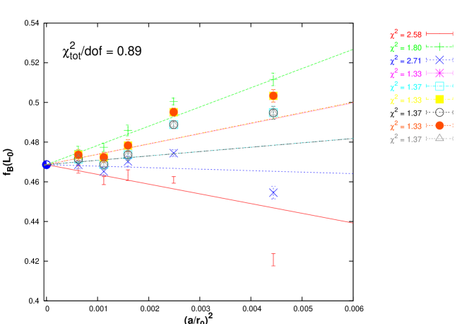
Figure 1: Continuum extrapolation on the small volume of $f_{B_{s}}(L_{0})$. The different values of the decay constant correspond to different definitions of the RGI quark masses given in equations (11), (12) and (13). For each definition the two points at largest lattice spacing has been shown but not included in the fit. Units are in GeV.

4.1 Small volume decay constants ($L_{0}=0.4$ fm)

Simulations of the decay constants on the smallest volume ($L_{0}=0.4$ fm) have been performed at five different lattice spacings using the geometries $24\times 12^{3}$, $32\times 16^{3}$, $40\times 20^{3}$, $48\times 24^{3}$ and $64\times 32^{3}$. For each discretization, a set of eight quark masses have been simulated. Two of the heavy masses have been chosen around the bottom quark $m^{RGI}_{b}=6.73(16)$ GeV [29]. Other two have been chosen in the region of the charm quark $m_{c}^{RGI}=1.681(36)$ [29]. An additional heavy quark has been simulated with mass $4.00$ GeV. Three light quark have been simulated with RGI masses of $0.14$ GeV, $0.10$ GeV and $0.06$ GeV. Using the accurate determination of the RGI strange quark mass given in [45] we have fixed one of the simulated light quarks to be the physical $s$. We will combine this finite volume calculations with the ones of the step scaling functions to provide results for the heavy–light decay constants with light quarks around the the strange in the continuum and on the large volume. All the parameters of the five different simulations are summarized in Table [1].

We have obtained different set of data by using the different definitions of the RGI quark masses given in the equations (11), (12) and (13). The continuum results are thus obtained trough a combined fit of all the set of data, linear in $(a/r_{0})^{2}$, as shown in Figure [1] in the case of the $\overline{b}s$ meson. For each set of data we have included in the fit the three points nearest to the continuum obtaining a global $\chi^{2}/dof=0.89$ to be compared with the $\chi^{2}$s of each individual definition listed in the figure. At this small volume, we are in a region of small bare couplings ($g_{0}^{2}\sim 0.85$) where it is legitimate to use perturbative values for the improvement coefficient $b_{A}$. The systematics introduced in the calculation by the continuum extrapolations have been estimated repeating the fits linear in $(a/r_{0})^{2}$ including, for each set of data, only the two points nearest to the continuum. We find a deviation leading to a corresponding systematic error of the order of $1$% that will be given to the results on the large volume added in quadrature with an error of about $2$% coming from the uncertainties on the lattice spacing and on the renormalization factors. The latter have been evaluated by moving the points as a consequence of the change, within the errors, of the lattice spacings and of the renormalization constants and by repeating the whole analysis.

The numbers we obtain are:

$$f_{B_{s}}(L_{0})=475(2)MeV\qquad f_{D_{s}}(L_{0})=644(3)MeV$$ (18)

The errors quoted at this stage are statistical only, evaluated by a jackknife procedure.
Due to the compression of the low energy scale, these results are higher than the large volume ones obtained after the step scaling functions multiplication chain (see eqs. (21),  (22) and  (23)).

4.2 First evolution step ($L_{0}\to L_{1}$)

$\beta$	$L_{0}/a$	$k_{c}$	$k$	$m^{RGI}$ (GeV)
			0.120674	3.543(39)
			0.122220	3.114(34)
			0.126937	1.927(21)
6.420	$8$	0.135703(9)	0.134304	0.3007(36)
			0.134770	0.2003(28)
			0.135221	0.1028(21)
			0.1249	3.542(39)
			0.1260	3.136(34)
			0.1293	1.979(22)
6.737	$12$	0.135235(5)	0.1343	0.3127(38)
			0.1346	0.2090(28)
			0.1349	0.1080(21)
			0.127074	3.549(39)
			0.127913	3.153(35)
			0.130409	2.003(22)
6.963	$16$	0.134832(4)	0.134145	0.3134(38)
			0.134369	0.2112(28)
			0.134593	0.1086(20)

Table 2: Simulation parameters for the first evolution step $L_{0}\to L_{1}=0.8$ fm. The RGI quark masses are obtained using eq. (11).

Figure 2: The figure shows the step scaling functions $\Sigma(L_{0})$ as functions of $m_{1}^{RGI}$, for the simulation of the first evolution step corresponding to $\beta=6.963$. The different sets of data correspond to the values of $m_{2}^{RGI}$. As can be seen the step scaling functions approach a plateau for high values of $m_{1}^{RGI}$. Similar plots can be obtained for the other values of the bare couplings.

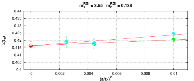
Figure 3: Continuum extrapolation on the first evolution step, $L_{0}\mapsto L_{1}$, of the step scaling function, $\Sigma(L_{0})$, of the pseudoscalar meson corresponding to the heavy quark of mass $m_{1}^{RGI}=3.55$ GeV and to the $s$–quark. The two sets of data are obtained using the two definitions of RGI quark masses of equations (11) and (13). Units are in GeV. Similar plots can be obtained for the other combinations of quark masses used in our simulations.

Figure 4: The figure shows the continuum extrapolated step scaling functions $\sigma(L_{0})$ as functions of $1/m_{1}^{RGI}$. The heavy extrapolations are shown only for the $\overline{h}s$ set of data.

The finite volume effects on the decay constants calculated on $L_{0}$, are measured by doubling the volume, $L_{1}=0.8$ fm, and by using the step scaling function of eq (2).

The continuum extrapolations have been obtained by simulating the step scaling functions with three different discretizations of $L_{0}$, i.e $16\times 8^{3}$, $24\times 12^{3}$ and $32\times 16^{3}$. The volume $L_{1}$ has been simulated starting from the discretizations of $L_{0}$, fixing the value of the bare coupling and doubling the number of lattice points in each direction.

The simulated quark masses have been halved with respect to the masses simulated on the small volume in order to have the same amount of the discretization effects proportional to $am$. The set of parameters for the simulations of this evolution step is reported in Table [2].
The step scaling functions at $\beta=6.963$ are plotted, at fixed $m^{RGI}_{2}$, as functions of $m^{RGI}_{1}$ in Figure [2]. As can be seen, $\Sigma(L_{0})$ is almost flat in a region of heavy quark masses starting around the charm mass. The hypothesis of low sensitivity upon the high–energy scale is thus verified. The value of the step scaling functions for the $s$ quark are obtained trough linear interpolation.
In Figure [3] are reported the results of the continuum extrapolation of the step scaling function, $\Sigma(L_{0})$, of the pseudoscalar $\overline{h}s$ meson corresponding to the heaviest quark simulated in this step ($m_{h}^{RGI}=3.55$ GeV).
The residual heavy mass dependence of the continuum extrapolated step scaling functions is very mild, as shown in Figure [4] in the plot of $\sigma_{B_{s}}$ as a function of the inverse quark mass. The continuum results are linearly extrapolated at the values of the heavy quark masses used in the small volume simulations.

The numbers we get at this step are:

$$\sigma_{B_{s}}(L_{0})=0.417(3)\qquad\sigma_{D_{s}}(L_{0})=0.414(3)$$ (19)

The step scaling functions are free from the systematic errors coming from uncertainties on $Z_{A}$ and $b_{A}$ since the multiplicative improvement and renormalization factors cancel exactly in the ratio, being the numerator and the denominator evaluated at the same lattice spacing.

4.3 Second evolution step ($L_{1}\to L_{2}$)

$\beta$	$L_{1}/a$	$k_{c}$	$k$	$m^{RGI}$ (GeV)
			0.118128	2.012(22)
			0.121012	1.551(17)
			0.122513	1.337(15)
5.960	$8$	0.13490(4)	0.131457	0.3154(36)
			0.132335	0.2322(28)
			0.133226	0.1466(44)
			0.124090	1.984(22)
			0.126198	1.584(17)
			0.127280	1.389(15)
6.211	$12$	0.135831(8)	0.133574	0.3493(39)
			0.134177	0.2550(29)
			0.134786	0.1510(19)
			0.126996	1.933(21)
			0.128646	1.547(17)
			0.129487	1.355(14)
6.420	$16$	0.135734(5)	0.134318	0.3016(34)
			0.134775	0.2038(24)
			0.135235	0.1055(15)

Table 3: Simulation parameters for the first evolution step $L_{1}\to L_{2}=1.6$ fm. The RGI quark masses are obtained using eq. (11).

Figure 5: The figure shows the step scaling functions $\Sigma(L_{1})$ as functions of $m_{1}^{RGI}$, for the simulation of the first evolution step corresponding to $\beta=6.420$. The different sets of data correspond to the values of $m_{2}^{RGI}$. As can be seen the step scaling functions approach a plateau for high values of $m_{1}^{RGI}$. Similar plots can be obtained for the other values of the bare couplings.

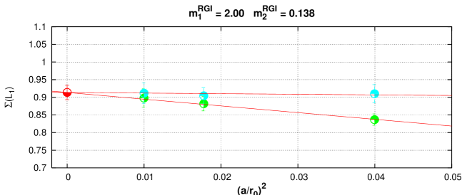
Figure 6: Continuum extrapolation on the first evolution step, $L_{1}\mapsto L_{2}$, of the step scaling function, $\Sigma(L_{1})$, of the pseudoscalar meson corresponding to the heavy quark of mass $m_{1}^{RGI}=2.00$ GeV and to the $s$–quark. The two sets of data are obtained using the two definitions of RGI quark masses of equations (11) and (13). Units are in GeV. Similar plots can be obtained for the other combinations of quark masses used in our simulations.

Figure 7: The figure shows the continuum extrapolated step scaling functions $\sigma(L_{1})$ as functions of $1/m_{1}^{RGI}$. The heavy extrapolations are shown only for the $\overline{h}s$ set of data.

In order to have the results on a physical volume, $L_{2}=1.6$ fm, a second evolution step is necessary. This is done computing the step scaling functions of eq. (2) at $L=L_{1}$, by the procedure outlined in the previous section. The parameters of the simulations are given in Table [3].

Also in this case, the values of the simulated quark masses have been halved with respect to the previous step, owing to the lower values of the simulation cutoffs. Even if we are lowering again the values of the quark masses, the linear extrapolations at the values of the heavy quark masses used on the small volume appears to be still valid and under control; see Figure [5,7].
The value of the step scaling functions for the $s$ quark are obtained trough linear interpolation.
Figure [6] shows the continuum extrapolation of the step scaling function, $\Sigma(L_{1})$, of the $\overline{h}s$ meson corresponding to the heaviest quark simulated in this step ($m_{h}^{RGI}=2.00$ GeV).

The numbers for this step are:

$$\sigma_{B_{s}}(L_{1})=0.97(3)\qquad\sigma_{D_{s}}(L_{1})=0.90(2)$$ (20)

5 Physical results

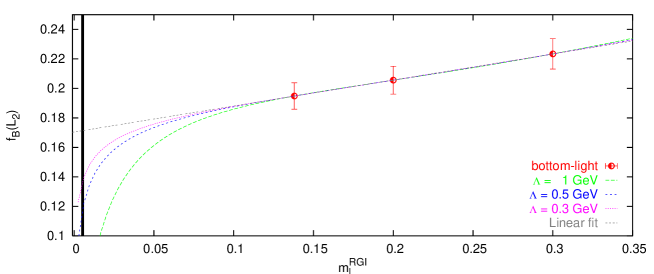
Figure 8: Chiral extrapolation of the continuum results for the pseudoscalar decay constants on the large volume. Units are in GeV.

In this section we combine the results of the small volume with the results of the step scaling functions to obtain, according to eq. (1), the physical numbers. In the end, we get:

$$f_{B_{s}}=192(6)(4)\ \mbox{MeV}\qquad f_{D_{s}}=240(5)(5)\ \mbox{MeV}$$ (21)

The first error is statistical while the second one is our estimate of the systematics due to the uncertainties on the continuum extrapolations, on the scale and on the renormalization factors, as already discussed in sec. 4.1.
Note that our value for $f_{D_{s}}$ agrees with the average of dedicated calculations performed on large volumes [15, 16]. This validates our choice of stopping at $L=1.6$ fm that, of course, can be explicitly checked to be safe by performing further evolution steps.
Using the strategy outlined in the previous sections, we have calculated also the decay constant of the $B_{c}$ meson. The result we obtain is

$$f_{B_{c}}=347(5)(8)\ \mbox{MeV}$$ (22)

that represents the first determination of this quantity from quenched lattice QCD.

The chiral behavior of heavy–light pseudoscalar decay constants has been shown [46, 47, 48, 49] to contain logarithmic terms ($\chi$–logs) that are diverging in the chiral limit, at variance with the unquenched case where these terms only affect the form of the extrapolation.
In Figure [8] we show the chiral extrapolations for the continuum heavy–light pseudoscalar decay constants. The data corresponding to the different values of the parameter $\Lambda$ have been extrapolated using the parametrization suggested in [49]. As can be seen from the figure, the presence of the unphysical quenched $\chi$–logs make the extrapolations unreliable down to the $u$–quark mass while the strange region seems to be dominated by a linear behavior. Nevertheless, in the literature values extrapolated linearly in the light quark mass have been quoted.
For a historical comparison we can quote our own:

$$f_{B}^{linear}=171(8)(4)\ \mbox{MeV}\qquad f_{D}^{linear}=221(7)(5)\ \mbox{MeV}$$

$$\frac{f_{B_{s}}}{f_{B}^{linear}}=1.12(2)(1)\qquad\frac{f_{D_{s}}}{f_{D}^{linear}}=1.09(1)(1)$$ (23)

that differ by a large factor from the unreliable values obtained from the fits shown in Figure [8] because of the diverging $\chi$–logs. The numbers quoted above should then be retained for an historical comparison only and should not be quoted as the results of the quenched approximation.

6 Conclusions

In this work we have calculated the $B_{s}$–meson decay constant in the continuum limit of quenched lattice QCD. The results are obtained through a finite volume recursive procedure where the heavy quark masses have been obtained, using the same method, in a previous work.

The main achievement of this computation with respect to our previous determination of the same quantities are the extrapolations to the continuum limit. Our systematic errors are due to the extrapolations to the continuum and to the physical heavy quark masses. An additional unknown systematics comes from the quenched approximation that is believed to produce visible effects on the meson decay constants. The known pathological behavior of quenched $\chi$–QCD does not allow us to quote a quenched value for $f_{B}$.

Upcoming new powerful super-computers will make affordable straight calculations of lattice $b$–physics without recursive methods but still in the quenched approximation. In this scenario our method could provide the opportunity of studying unquenched $b$–physics and/or to deal with other demanding two–scales problems.

References

- [1] M. Ciuchini et al., JHEP 07 (2001) 013, hep-ph/0012308.
- [2] A. Hocker et al., Eur. Phys. J. C21 (2001) 225, hep-ph/0104062.
- [3] A.J. Buras, F. Parodi and A. Stocchi, (2002), hep-ph/0207101.
- [4] A. Stocchi, (2002), hep-ph/0211245.
- [5] D.J. Broadhurst and A.G. Grozin, Phys. Lett. B274 (1992) 421, hep-ph/9908363.
- [6] E. Bagan et al., Phys. Lett. B278 (1992) 457.
- [7] M. Neubert, Phys. Rev. D45 (1992) 2451.
- [8] T.M. Aliev and V.L. Eletsky, Sov. J. Nucl. Phys. 38 (1983) 936.
- [9] C.A. Dominguez and N. Paver, Phys. Lett. 197B (1987) 423.
- [10] S. Narison, Phys. Lett. B198 (1987) 104.
- [11] L.J. Reinders, Phys. Rev. D38 (1988) 947.
- [12] P. Colangelo et al., Phys. Lett. B269 (1991) 201.
- [13] A.A. Penin and M. Steinhauser, Phys. Rev. D65 (2002) 054006, hep-ph/0108110.
- [14] M. Jamin and B.O. Lange, Phys. Rev. D65 (2002) 056005, hep-ph/0108135.
- [15] N. Yamada, (2002), hep-lat/0210035.
- [16] D. Becirevic, (2002), hep-ph/0211340.
- [17] D. Becirevic et al., Phys. Rev. D60 (1999) 074501, hep-lat/9811003.
- [18] C.W. Bernard et al., Phys. Rev. Lett. 81 (1998) 4812, hep-ph/9806412.
- [19] CP-PACS, A. Ali Khan et al., Phys. Rev. D64 (2001) 034505, hep-lat/0010009.
- [20] UKQCD, K.C. Bowler et al., Nucl. Phys. B619 (2001) 507, hep-lat/0007020.
- [21] UKQCD, L. Lellouch and C.J.D. Lin, Phys. Rev. D64 (2001) 094501, hep-ph/0011086.
- [22] MILC, C. Bernard et al., Phys. Rev. D66 (2002) 094501, hep-lat/0206016.
- [23] ALPHA, M. Kurth and R. Sommer, Nucl. Phys. B597 (2001) 488, hep-lat/0007002.
- [24] J. Heitger, M. Kurth and R. Sommer, (2003), hep-lat/0302019.
- [25] JLQCD, K.I. Ishikawa et al., Phys. Rev. D61 (2000) 074501, hep-lat/9905036.
- [26] CP-PACS, A. Ali Khan et al., Phys. Rev. D64 (2001) 054504, hep-lat/0103020.
- [27] A.X. El-Khadra et al., Phys. Rev. D58 (1998) 014506, hep-ph/9711426.
- [28] M. Guagnelli et al., Phys. Lett. B546 (2002) 237, hep-lat/0206023.
- [29] G.M. de Divitiis et al., (2003), hep-lat/0305018.
- [30] J. Gasser and H. Leutwyler, Nucl. Phys. B250 (1985) 465.
- [31] S. Capitani et al., Nucl. Phys. Proc. Suppl. 63 (1998) 153, hep-lat/9709125.
- [32] ALPHA, M. Guagnelli, R. Sommer and H. Wittig, Nucl. Phys. B535 (1998) 389, hep-lat/9806005.
- [33] S. Necco and R. Sommer, Nucl. Phys. B622 (2002) 328, hep-lat/0108008.
- [34] M. Guagnelli, R. Petronzio and N. Tantalo, Phys. Lett. B548 (2002) 58, hep-lat/0209112.
- [35] M. Luscher et al., Nucl. Phys. B384 (1992) 168, hep-lat/9207009.
- [36] S. Sint, Nucl. Phys. B421 (1994) 135, hep-lat/9312079.
- [37] M. Luscher et al., Nucl. Phys. B413 (1994) 481, hep-lat/9309005.
- [38] ALPHA, A. Bode et al., Phys. Lett. B515 (2001) 49, hep-lat/0105003.
- [39] Zeuthen-Rome / ZeRo, M. Guagnelli et al., (2003), hep-lat/0303012.
- [40] M. Luscher et al., Nucl. Phys. B491 (1997) 323, hep-lat/9609035.
- [41] M. Luscher et al., Nucl. Phys. B491 (1997) 344, hep-lat/9611015.
- [42] S. Sint and P. Weisz, Nucl. Phys. B502 (1997) 251, hep-lat/9704001.
- [43] G.M. de Divitiis and R. Petronzio, Phys. Lett. B419 (1998) 311, hep-lat/9710071.
- [44] ALPHA, M. Guagnelli et al., Nucl. Phys. B595 (2001) 44, hep-lat/0009021.
- [45] ALPHA, J. Garden et al., Nucl. Phys. B571 (2000) 237, hep-lat/9906013.
- [46] C.W. Bernard and M.F.L. Golterman, Phys. Rev. D46 (1992) 853, hep-lat/9204007.
- [47] S.R. Sharpe, Phys. Rev. D46 (1992) 3146, hep-lat/9205020.
- [48] M.J. Booth, Phys. Rev. D51 (1995) 2338, hep-ph/9411433.
- [49] S.R. Sharpe and Y. Zhang, Phys. Rev. D53 (1996) 5125, hep-lat/9510037.