Quenched charmonium spectrum

QCD-TARO Collaboration: S. Choe^a, Ph. de Forcrand^b,c, M. García Pérez^d, Y. Liu^e, A. Nakamura^f, I.-O. Stamatescu^g,h, T. Takaishiⁱ and T. Umeda^k

^a Department of Chemistry, KAIST, 373-1 Kusung-dong, Yusung-gu, Daejon 305-701, Korea
^b Institut für Theoretische Physik, ETH-Hönggerberg, CH-8093 Zürich, Switzerland
^c Theory Division, CERN, CH-1211 Geneva 23, Switzerland
^d Instituto de Física Teórica, Universidad Autónoma de Madrid, Cantoblanco, 28049 Madrid, Spain
^e Department of Physics, Nakai University, Tianjin 300071, China
^f IMC, Hiroshima University, Higashi-Hiroshima 739-8521, Japan
^g Institut für Theoretische Physik, Universität Heidelberg, D-69120 Heidelberg, Germany
^h FEST, Schmeilweg 5, D-69118 Heidelberg, Germany
ⁱ Hiroshima University of Economics, Hiroshima 731-0192, Japan
^j Yukawa Institute for Theoretical Physics, Kyoto University, Japan

We study charmonium using the standard relativistic formalism in the quenched approximation, on a set of lattices with isotropic lattice spacings ranging from 0.1 to 0.04 fm. We concentrate on the calculation of the hyperfine splitting between $\eta_{c}$ and $J/\psi$, aiming for a controlled continuum extrapolation of this quantity. The splitting extracted from the non-perturbatively improved clover Dirac operator shows very little dependence on the lattice spacing for $a\leq 0.1$fm. The dependence is much stronger for Wilson and tree-level improved clover operators, but they still yield consistent extrapolations if sufficiently fine lattices, $a\leq 0.07$ fm ($aM(\eta_{c})\leq 1$), are used. Our result for the hyperfine splitting is $77(2)(6)$ MeV (where Sommer’s parameter, $r_{0}$, is used to fix the scale). This value remains about 30$\%$ below experiment. Dynamical fermions and OZI-forbidden diagrams both contribute to the remainder. Results for the $\eta_{c}$ and $J/\psi$ wave functions are also presented.

1 Introduction

Heavy QCD quarkonium systems have been thoroughly studied analytically within the heavy quark non-relativistic approximation, NRQCD [2], and related heavy quark effective theories as pNRQCD [3] and vNRQCD [4]– for a recent review see [5]. These approaches, however, generically fail for charmonium. For $c\bar{c}$ the expansion parameter $v^{2}\!/\!c^{2}$ of the effective theory is about $0.3$, and higher order corrections in $v/c$ seemingly become very large, even overwhelming the leading order terms. It is particularly challenging to reproduce the hyperfine splitting between the $\!\!\ {}^{3}S_{1}$ and the $\!\!\ {}^{1}S_{0}$ states, which for charmonium is $M(J/\psi-\eta_{c})=117$ MeV. The lattice version of NRQCD predicts a value of the hyperfine splitting $M(J/\psi-\eta_{c})=\!55(5)$ MeV [6] far below the experimental value, although still quite remarkable taking into account all the approximations involved. Indeed lattice NRQCD, being an effective action with cutoff given by the heavy quark mass $m_{q}$, does not allow for a continuum extrapolation: for the effective action to be valid one has to preserve $am_{q}>1$. Given this, the estimation of the systematic uncertainties inherent in the discretization is quite difficult. This fact, together with the observation that the $v/c$ expansion is not well justified for charmonium, encourages the suspicion that the origin of the discrepancy between experimental and computed hyperfine splitting could lie in the non-relativistic approximation. However, all other lattice determinations based on relativistic actions also underestimate the value of the hyperfine splitting, by as much as $30\!-\!50\%$ [7, 8, 9, 10, 11]. This raises what one might call the puzzle of the hyperfine splitting.

Almost all lattice calculations up to now, including NRQCD, have been performed within the quenched (valence quark) approximation (for recent reviews on heavy quarks on the lattice see [12, 13]). The effect of quenching has been estimated [14] by looking at the predicted form of the hyperfine splitting in the heavy quark approximation

$$M(J/\psi-\eta_{c})=\frac{32\pi\alpha_{s}(m_{q})}{9m_{q}^{2}}|\Psi(0)|^{2}\quad,$$ (1)

with $\Psi(0)$ the value of the non-relativistic wave function at the origin. In Ref. [14] it is argued that the change in $\Psi(0)$ and in the running of $\alpha_{s}$ due to dynamical quarks can give altogether a deviation of the quenched result from the real world case as large as $40\%$. This would make the hyperfine splitting a quantity particularly suitable for unveiling unquenching effects – typically the effects of quenching on other spectral quantities amount to only $\sim 10\%$. However, first numerical results including dynamical quarks seem to indicate a much milder $N_{f}$ dependence of the hyperfine splitting than what is needed to match the experimental result [15, 16]. This raises some worry about the reliability of the calculations performed up to now, in particular since they have been typically done at not so small values of the lattice spacing. This worry becomes more severe after noting that continuum extrapolations of the hyperfine splitting seem to depend quite strongly on the kind of Dirac operator used for the calculation [6, 10, 15]. Needless to say that the continuum limit is unique. Such strong dependence on the choice of Dirac operator has to reflect the existence of large lattice artifacts.

Indeed, the reason why a reliable determination of the hyperfine splitting by means of purely non-perturbative relativistic calculations remains elusive is that charm is too heavy for most current lattice simulations. For charm the dominant lattice artifacts are of ${\cal O}((am_{c})^{n}),\ n\geq 1$, with $am_{c}\sim 0.5$ at the typical values of the lattice spacing. Lattice artifacts remain large and may completely spoil the determination of the charmonium spectrum.

One particular approach that has been advocated in order to avoid large ${\cal O}(am_{q})$ lattice artifacts for heavy quark systems is the use of anisotropic lattices [8]. Such lattices [17] have different lattice spacings $a_{s}$ and $a_{t}$ in spatial and temporal directions, with $a_{t}<<a_{s}$. In Ref. [8] it has been argued that by tuning appropriately the parameters of the action one could achieve reduced scaling violations of $O((a_{t}m_{q})^{n})$ while keeping still $a_{s}m_{q}$ large. This is certainly a very attractive possibility, which would make anisotropic lattices quite advantageous over standard isotropic ones. In particular this is the approach that has been taken in several recent studies of the charmonium spectrum [8, 9, 10, 11, 20]. However, recent analysis seem to point out that scaling violations governed by the large $a_{s}m_{q}$ artifacts could revive at the one loop level [18, 19]. This casts doubt on the generic effectiveness of anisotropic actions in reducing lattice artifacts better than standard isotropic lattices. To settle this point, an analysis of the range of validity of the anisotropic approach, as performed in [21], seems essential.

Our methodology here is to compute $M(J/\psi-\eta_{c})$ on very fine isotropic lattices within the quenched relativistic formalism. If the lattices used are sufficiently fine, this approach should allow for a controlled quenched continuum extrapolation, free of the systematic uncertainties which may have affected other determinations up to now. Particularly important for this will be the use of a non-perturbatively improved version of the Dirac operator, for which lattice artifacts are reduced to ${\cal O}((am_{q})^{2})$. Preliminary results of this calculation have been presented in [22].

We want to stress that our calculation, which does not differ from any other in this respect, involves one other approximation besides quenching: OZI, meaning that Zweig-rule forbidden diagrams are not taken into account. Such diagrams, as in Fig. 1, contribute to the correlator of flavor singlet mesons like charmonium. They have been particularly studied for light quarks in connection with the U(1)_A symmetry breaking and the $\eta^{\prime}$ mass, where the anomaly provides an enhancement of OZI contributions to pseudoscalar mesons - for lattice estimates see [23, 24]. There is however no lattice calculation of their magnitude for heavy quarkonium states like charmonium. In the quark model [25, 26] these OZI amplitudes are expected to be proportional to the value of the wave function at the origin, and hence are suppressed for P-wave channels which have vanishing wave function at $\vec{r}=\vec{0}$. For S-wave, their contribution is ${\cal O}(\alpha_{s}^{2}(m_{PS}))$ and ${\cal O}(\alpha_{s}^{3}(m_{V}))$ suppressed for the pseudo-scalar and vector channels respectively. Experimental evidence of the goodness of the OZI rule and of this relative suppression comes from the hadronic widths of heavy pseudo-scalar and vector mesons. The effect of these diagrams is therefore expected to be small for heavy quark systems like charmonium. Here, we neglect such “disconnected” diagrams because of their high computer cost. We want to stress, however, that their contribution may amount to several MeV, perhaps a not so negligible effect given the small value of the hyperfine splitting. Moreover, the OZI contribution could be enhanced by mixing with glueballs with the appropriate quantum numbers provided these glueballs were almost degenerate in mass with the charmonium states, an effect that has been measured for light singlet mesons [23, 27].

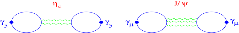
Figure 1: Zweig rule forbidden diagrams contributing to the pseudoscalar (Left) and vector (Right) channels. These closed quark loops are connected by gluonic contributions, of which we only show those that contribute to lowest order in $\alpha_{s}$.

The paper is organized as follows. Section 2 compiles our results. In Section 2.1 details about our numerical simulations are presented, including the kind of Dirac operators used to measure meson masses and the strategy to extract the hyperfine splitting from 2-point correlators. In Section 2.2 we give our values for the $\!\!\ {}^{3}S_{1}-\!\!\ ^{1}S_{0}$ hyperfine splitting as well as the $1P$ to $\!\!\ {}^{3}S_{1}$ splittings, obtained with the non-perturbatively improved clover Dirac operator. Our continuum extrapolation of the charmonium spectrum is based on data at lattice spacings ranging from $a=0.0931$ fm to 0.0397 fm. A comparison with the results obtained from Wilson and tree-level clover Dirac operators is given in Section 2.3. In Section 2.4 we present the results for the $\eta_{c}$ and $J/\psi$ wave functions. We investigate the volume dependence or our results in Section 2.5, by looking at the dependence on physical volume of both the spectrum and the wave functions. Finally, our summary and conclusions are presented in Section 3.

2 Results

We have aimed at analyzing the S- and P-wave states indicated in Table 1. Precise results will only be presented for the $\!\!\ {}^{3}S_{1}-\!\!\ ^{1}S_{0}$ hyperfine splitting, although preliminary results for P-wave meson masses will also be given.

Table 1: Charmonium S- and P-wave states analyzed in this work. We indicate their quantum numbers and physical masses. Unless indicated experimental errors are one or less in the last indicated digit.

Name	${}^{(2s+1)}L_{J}$	$J^{PC}$	Mass(GeV)
$\eta_{c}$	${}^{1}S_{0}$	$0^{-+}$	2.980(2)
$J/\psi$	${}^{3}S_{1}$	$1^{--}$	3.097
$h_{c}$	${}^{1}P_{1}$	$1^{+-}$	3.526
$\chi_{c0}$	${}^{3}P_{0}$	$0^{++}$	3.415
$\chi_{c1}$	${}^{3}P_{1}$	$1^{++}$	3.511

2.1 Simulation details

Gauge configurations are generated with the standard Wilson action. Simulation parameters - see Table 2 - have been chosen so as to fix a physical lattice size of about 1.6 fm. In addition we have also simulated a very fine $32^{3}\times 96$ lattice at $\beta=6.6$, corresponding to a smaller size of 1.3 fm (possible finite volume effects will be discussed in section 2.5). The physical scale is set by $r_{0}$ from [28].

Table 2: Simulation parameters. The scale is set by $r_{0}$ from [28]. The non-perturbative value of the clover coefficient, $c_{sw}^{\rm NP}$, has been computed in [29].

$\beta$	$L^{3}\times T$	$a({\rm fm})$	$La({\rm fm})$	$c_{sw}^{\rm NP}$	$\#$ conf.
6.0	$18^{3}\times 48$	0.0931	1.68	1.769	190
6.2	$24^{3}\times 72$	0.0677	1.62	1.614	90
6.4	$32^{3}\times 96$	0.0513	1.64	1.526	60
6.6	$32^{3}\times 96$	0.0397	1.27	1.467	130

Quark propagators are computed using Wilson, tree-level clover and non- perturbatively improved clover Dirac operators. The non-perturbative value of the clover coefficient is taken from [29].

A complete analysis of the spectrum, at all $\beta$ values, has only been performed for the non-perturbatively improved clover Dirac operator. For Wilson and tree-level clover Dirac operators we have results at $\beta=6.2$ (for Wilson), $\beta=6.4$ and $\beta=6.6$. The continuum extrapolations in such cases are based on available data at $\beta\!=\!6.0$ and 6.2 from UKQCD [7, 30].

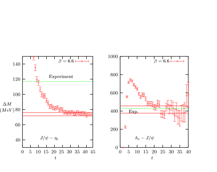
Figure 2: Left: $\!\!\ {}^{3}S_{1}-\!\!\ ^{1}S_{0}$ hyperfine splitting effective mass. Right: ${}^{1}P_{1}-\!\!\ ^{3}S_{1}$ splitting effective mass. Data are obtained using the non-perturbatively improved clover Dirac operator. The dashed horizontal line is the experimental value and the band comprises our fit to a constant with its errors.

We compute correlation functions of hadronic operators with zero-momentum point source and point sink. A time dependent effective mass $M(t)$ is extracted by fitting the ratio of correlators at a pair of points ($t$, $t+1$) to:

$$R(t)\equiv\frac{\langle C(t)\rangle}{\langle C(t+1)\rangle}=\frac{{\rm cosh}[(\frac{T}{2}-t)\ M(t)]}{{\rm cosh}[(\frac{T}{2}-t-1)\ M(t)]}.$$ (2)

Here $\langle.\rangle$ means summation over Yang-Mills configurations. The plateau in the effective mass is then fitted to a constant which provides our estimate of the meson mass.

In addition, we extract mass differences between the states in Table 1 from the ratio of correlators, which behaves as:

$$\frac{R_{A}(t)}{R_{B}(t)}=\frac{{\rm cosh}[(\frac{T}{2}-t)M_{A}(t)]\ {\rm cosh}[(\frac{T}{2}-t-1)M_{B}(t)]}{{\rm cosh}[(\frac{T}{2}-t)M_{B}(t)]\ {\rm cosh}[(\frac{T}{2}-t-1)M_{A}(t)]}\ \ \sim_{{}_{{}_{\!\!\!\!\!\!\!\!\!\!\!\!T\rightarrow\infty}}}e^{-\Delta M(t)}\quad,$$ (3)

if the correlators are dominated by a single pole. This allows to extract a time dependent effective mass for the splitting, $\Delta M(t)\equiv M_{B}(t)-M_{A}(t)$, which is fitted to a constant in the range where the effective mass plateau sets in. The quality of the data for the hyperfine splitting is shown in Fig. 2 left. A similar plot for the ${}^{1}P_{1}-\!\!\ ^{3}S_{1}$ splitting is presented in Fig. 2 right. Although the signal extracted from Eq. (3) is less noisy than the one from Eq. (2), point sources are still too noisy for P-wave states and, within our statistics, do not allow a precise determination of the masses.

2.2 Charmonium spectrum from non-perturbatively
improved clover Dirac operator

We present first the results obtained with the non-perturbatively improved clover Dirac operator, for which scaling violations in spectral quantities are expected to be ${\cal O}(a^{2})$. A detailed comparison with Wilson and tree-level clover Dirac operators will be presented in section 2.3.

Table 3: Charmonium spectrum from non-perturbatively improved clover Dirac operator. Results are given in MeV with the scale set by $r_{0}$ from [28]. $\kappa$ has been tuned to maintain an approximately constant mass $M(\!\!\ ^{3}S_{1})\!\approx\!3095$ MeV $\forall a$. The last two columns show our continuum extrapolation and the experimental value.

	$\beta=6.0$	$\beta=6.2$	$\beta=6.4$	$\beta=6.6$	$a\rightarrow 0$	Exp.
	$\kappa=0.11865$	$\kappa=0.12457$	$\kappa=0.12755$	$\kappa=0.12943$
$\!\!\ {}^{1}S_{0}$	3023(2)	3019(3)	3034(3)	3014(3)		2980
$\!\!\ {}^{3}S_{1}$	3091(2)	3093(3)	3109(4)	3085(3)		3097
$\!\!\ {}^{3}S_{1}-\!\!\ ^{1}S_{0}$	68.5(1.3)	74.2(1.5)	75.2(2.5)	73.8 (2.1)	77.2(1.7)	$\ 117$
${}^{1}P_{1}-\!\!\ ^{3}S_{1}$	417(25)	460(34)	433(37)	417(40)	441(25)	429
${}^{3}P_{0}-\!\!\ ^{3}S_{1}$	342(19)	352(25)	369(34)	397(41)	387(14)	318
${}^{3}P_{1}-\!\!\ ^{3}S_{1}$	390(19)	413(34)	451(41)	417(29)	437(16)	414

We have used two different ways of setting the charm quark point: imposing that either $r_{0}M(\!\!\ ^{1}S_{0})$ or $r_{0}M(\!\!\ ^{3}S_{1})$ equals the physical value. These two different choices allow to study the ambiguities in the scale determination induced by the approximations we have made: quenched and OZI. We want to stress again that our calculation is affected not only by quenching ambiguities but also by OZI effects, i.e. only a subset of the relevant quenched diagrams has been included. Taking this into account we expect the choice of $J/\psi$ mass as reference to be a better one, since in that case OZI contributions to the $J/\psi$ mass are expected to be considerably suppressed compared to the pseudoscalar ones - see for instance [34] and the discussion in Section 1. For these reason the numbers presented here refer to the choice of $J/\psi$ mass as reference. The hyperfine splitting with $M(\!\!\ ^{1}S_{0})$ fixed to the experimental $\eta_{c}$ value will be used below when we estimate the systematic uncertainty in our calculation. An alternative possibility, which we have not explored, would be to fix the charm quark point by using the $D_{s}$ meson mass, as done for instance in heavy-light spectroscopy and for the determination of the charm quark mass [31, 32]. This would be free of OZI ambiguities.

Our results are collected in Table 3. As indicated above, the charm quark point has been obtained by fixing $M(\!\!\ ^{3}S_{1})\approx 3095$ MeV for all $a$. We compute the hyperfine splitting from: $(A)$ the difference between the $\!\!\ {}^{3}S_{1}$ and $\!\!\ {}^{1}S_{0}$ masses and $(B)$ the hyperfine splitting effective mass extracted from the ratio of correlators Eq. (3). Both determinations are perfectly consistent within errors but (B) is more precise and will be used henceforth. Fig. 3 shows the results for the $\!\!\ {}^{3}S_{1}-\!\!\ ^{1}S_{0}$ hyperfine splitting as a function of $a^{2}$. The lattice spacing dependence is very small. On the coarsest lattice, for which $aM({\!\!\ {}^{1}S_{0}})\approx 1.4$ and large scaling violations could be expected, the deviation from our continuum extrapolation amounts to only $11\%$. The cutoff dependence is well fitted linearly in $a^{2}$. The continuum extrapolation is $M({\!\!\ {}^{3}S_{1}-\!\!\ ^{1}S_{0}})=77(2)$ MeV. Excluding from the fit the point at $\beta=6.0$ gives $M({\!\!\ {}^{3}S_{1}-\!\!\ ^{1}S_{0}})=74(1)$ MeV. If, instead of the vector mass, we fix the charm scale by setting $M(\!\!\ ^{1}S_{0})\approx 2.945$ MeV $\forall a$, the result for the hyperfine splitting goes up by $6\%$. Including both these results as systematic error in our determination we quote as value of the hyperfine splitting from the non-perturbatively improved clover Dirac operator $M({\!\!\ {}^{3}S_{1}-\!\!\ ^{1}S_{0}})=77(2)(6)$. This is about $30\%$ below the experimental value.

When comparing our number to previous lattice determinations - see [9, 10, 7, 6] - it is important to note that we have used $r_{0}$ to set the scale. It is is quite common for charmonium analysis to use instead the spin averaged splitting, $\ {}^{1}P_{1}-\overline{S}$ or $\overline{P}-\overline{S}$, which is claimed to lead to considerably larger values of the hyperfine splitting. Variations with the scale input are usually blamed on the quenched approximation . Although this is partially true, the large differences often quoted are also coming from large scaling violations. This has been already illustrated by the latest CP-PACS result [10], obtained using the Fermilab anisotropic action. The discrepancy in the determination of the hyperfine splitting from $r_{0}$ or $\overline{P}-\overline{S}$ has been reduced from 27 to 16$\%$ as the lattices used in the continuum extrapolation have changed from $a\in[0.099,0.208]$ fm [9] to $a\in[0.0697,0.1374]$ fm [10]. Their final number is $M({\!\!\ {}^{3}S_{1}-\!\!\ ^{1}S_{0}})_{\overline{P}-\overline{S}}=85.3(4.4)^{(+5.7)}_{(-2.5)}$ MeV. From $r_{0}$ they obtain instead $M({\!\!\ {}^{3}S_{1}-\!\!\ ^{1}S_{0}})_{r_{0}}=72.6(9)^{(+1.2)}_{(-3.8)}$ MeV (the previous result in [9] was $M({\!\!\ {}^{3}S_{1}-\!\!\ ^{1}S_{0}})_{r_{0}}=65(1)$ MeV, the discrepancy clearly reflecting the large systematic ambiguities due to scaling violations). Our final number, $M({\!\!\ {}^{3}S_{1}-\!\!\ ^{1}S_{0}})_{r_{0}}=77(2)(6)$, lies in between their two determinations, and is compatible within errors with both.

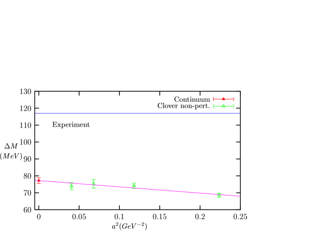
Figure 3: Continuum extrapolation of the hyperfine splitting with the non-perturbatively improved clover Dirac operator. The bare quark mass is tuned to maintain an approximately constant mass $M(\!\!\ ^{3}S_{1})\approx 3095$ MeV $\forall a$.

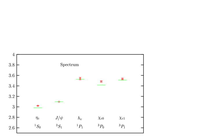
Figure 4: Comparison between the experimental charmonium spectrum and our numerical data. The scale is set by $r_{0}$. The value of the $J/\psi$ mass is fixed to the experimental one.

We have also computed the splitting between P-wave states and the $\!\!\ {}^{3}S_{1}$. Results are presented in Table 3. With point sources and within our limited statistics, our results are too noisy to attempt a reasonable continuum extrapolation and make a definite statement about scaling violations in these quantities. Still, our estimates of the $J=1$ to $J/\psi$ splittings are consistent, within errors, with experiment. The discrepancy turns out to be larger for the ${}^{3}P_{0}$ state.

An estimate of the ambiguities inherent in the quenched plus OZI approximations can be extracted from the values of the continuum extrapolated spectrum. Figure 4 presents a comparison between the experimental charmonium spectrum and our data. Deviations from experiment amount to $30\%$ for the $J/\psi$ to $\eta_{c}$ splitting, and $22\%$ for the ${}^{3}P_{0}$ to $J/\psi$ splitting. They are considerably reduced for the $J=1$, P-wave to $J/\psi$ splittings, which are consistent within errors with experiment.

2.3 Dependence on the choice of Dirac operator and continuum extrapolations.

As discussed in the Introduction, it has been often reported [6, 10, 15] that the continuum extrapolated hyperfine splitting strongly depends on the choice of Dirac operator. This happens in particular with anisotropic actions like the ones used in [8, 9, 10] which are claimed to reduce ${\cal O}(m_{q}a_{s})^{n}$ scaling violations to ${\cal O}(m_{q}a_{t})^{n},\ a_{t}\ll a_{s}$. Since the continuum limit is unique, such strong dependence on the choice of Dirac operator necessarily reflects the existence of large lattice artifacts. Indeed, CP-PACS, in Ref. [10], concludes that $m_{q}a_{s}<1$ is still certainly needed in order to obtain reliable continuum extrapolations with anisotropic lattices. This is not surprising, but it is an indication that anisotropic lattices might not, in general, succeed in removing scaling violations better than isotropic lattices do (indications that ${\cal O}(g^{2}m_{q}a_{s})$ indeed revive at the one-loop level have been reported in [18, 19]). As we will see next, even with the non-improved Wilson Dirac operator a reasonable estimate of the hyperfine splitting can be obtained if, but only if, lattices with spacing $a\leq 0.07$ fm, i.e. $aM(\!\!\ ^{1}S_{0})\leq 1$, are used.

Table 4: Pseudoscalar, vector mass and hyperfine splitting from Wilson and tree-level clover Dirac operator. Results are given in physical units (MeV) with the scale set by $r_{0}$.

Dirac Op.	$\kappa$	$\beta$	$\!\!\ {}^{1}S_{0}$	$\!\!\ {}^{3}S_{1}$	$\!\!\ {}^{3}S_{1}-\!\!\ ^{1}S_{0}$
Wilson	0.1380	6.2	2728(3)	2764(4)	35.2(1.2)
Wilson	0.1375	6.2	2788(3)	2821(3)	33.2(0.9)
Wilson	0.1365	6.2	2913(3)	2943(3)	30.4(0.9)
Wilson	0.1350	6.2	3099(4)	3125(4)	26.7(0.9)
Wilson	0.1389	6.4	2925(4)	2963(4)	38.4 (1.6)
Wilson	0.1380	6.4	3087(4)	3122(5)	35.4 (1.7)
Wilson	0.1371	6.4	3263(5)	3288(4)	28.5 (1.1)
Wilson	0.1415	6.6	2594(5)	2652(6)	60.4 (2.4)
Wilson	0.1400	6.6	2970(6)	3017(7)	48.3 (2.3)
Wilson	0.1385	6.6	3338(5)	3375(5)	39.1 (1.6)
Wilson	0.1375	6.6	3583(5)	3613(5)	32.3 (1.6)
Clover	0.1324	6.4	2931(4)	2996(5)	64.5 (2.8)
Clover	0.1320	6.4	3022(4)	3081(4)	59.2 (2.5)
Clover	0.1315	6.4	3129(4)	3189(5)	59.0 (2.4)
Clover	0.1335	6.6	2964(6)	3031(6)	68.9 (3.2)
Clover	0.1330	6.6	3116(6)	3180(6)	64.8 (3.0)
Clover	0.13225	6.6	3342(6)	3399(6)	58.9 (2.8)

The pseudoscalar mass and the hyperfine splitting from Wilson and tree-level clover Dirac operators are presented in Table 4. We only have data at $\beta=6.2$ (for Wilson), $\beta=6.4$ and $\beta=6.6$. To perform the continuum extrapolation we use $\beta\!=\!6.0$ and 6.2 data from UKQCD [7, 30]. Our strategy here has been slightly different than in the previous section. Instead of fine tuning the vector mass at each $\beta$ value, we interpolate from a range of masses around the physical $J/\psi$ mass. We fit the dependence of $M(\!\!\ ^{3}S_{1}-\!\!\ ^{1}S_{0})$ versus $1/M(\!\!\ ^{3}S_{1})$ at fixed $\beta$, and extract the value of the hyperfine splitting at the desired vector meson mass from the fit. This allows to extract the splitting at $M(\!\!\ ^{3}S_{1})=3.095$ GeV, the same vector meson mass which we fixed for the non-perturbatively improved Dirac operator.

Concerning the continuum extrapolations we expect scaling violations to be:

• ${\cal O}(a)$ for the Wilson Dirac operator.

• ${\cal O}(a^{2})$ and ${\cal O}(g^{2}a)$ for the tree-level clover Dirac operator.

These are the dominant contributions but, for very coarse lattices, sub-leading terms might also be important especially since they depend on $(am_{q})^{2}$. To test the approach to the continuum, we present in Fig. 5 the results of two different extrapolations:

1. Top figure 5: using the three largest $\beta$ values,

   • linearly in $a$ for the Wilson Dirac operator

   • linearly in $a^{2}$ for the tree-level clover Dirac operator

   

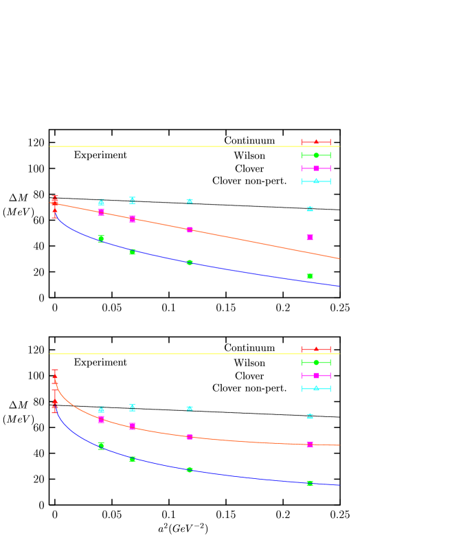
   Figure 5: Comparison between continuum extrapolation of $M(\!\!\ ^{3}S_{1}-\!\!\ ^{1}S_{0})$ with Wilson, tree-level clover and non-perturbatively improved clover Dirac operators. Top: Wilson and tree-level clover improved data are fitted linearly in $a$ and $a^{2}$ respectively. Bottom: Both Wilson and tree-level clover data are fitted with $a$ plus $a^{2}$ dependence. Wilson data at $\beta=6.0$ and tree level clover data at $\beta=6.0$ and $\beta=6.2$ are based on UKQCD results in [7, 30].

2. Bottom figure 5: using all four $\beta$ values,

   • including $a$ and $a^{2}$ terms for the Wilson Dirac operator

   • including $a$ and $a^{2}$ terms for the tree-level clover Dirac operator

We obtain as continuum extrapolations for the Wilson and tree-level clover respectively: $M(\!\!\ ^{3}S_{1}-\!\!\ ^{1}S_{0})=67(6)$ MeV and $73(1)$ MeV from fit (I) and $M(\!\!\ ^{3}S_{1}-\!\!\ ^{1}S_{0})=80(9)$ MeV and $99(5)$ MeV from fit (II). This is to be compared with the result from non-perturbative improvement $M({\!\!\ {}^{3}S_{1}-\!\!\ ^{1}S_{0}})=77(2)$ MeV.

Several remarks are in order here:

$(i)$ Only the non-perturbatively improved data show a weak dependence on the lattice spacing. Wilson and tree-level clover data are both significantly below their continuum extrapolations at all the simulated $\beta$ values.

$(ii)$ Linear extrapolations in $a$ and $a^{2}$ for Wilson and tree-level clover respectively, including $\beta\!=\!6.0$ ($aM({\!\!\ {}^{1}S_{0}})=1.4$) are not justified.

$(iii)$ If too coarse lattices are included in the fit, continuum extrapolations become quite sensitive to the assumed dependence on the lattice spacing. This is clearly observed in the case of the tree-level clover data, for which fit (II) gives a considerably higher continuum value. It is only when the extrapolations start from sufficiently fine lattices that they come out reasonably consistent. A lower bound for consistent extrapolations seems to be $a\leq 0.07$ fm for Wilson and tree-level clover data, i.e. $aM(\!\!\ ^{1}S_{0})\leq 1$. Surprisingly, though, non-perturbative clover improvement seems to work well even on the coarser $\beta=6.0$ lattice where $aM({\!\!\ {}^{1}S_{0}})=1.4$.

To summarize, non-perturbative clover improvement seems crucial to remove strong scaling violations. It is possible to extract comparable results from Wilson or tree-level clover improved Dirac operators, but very fine lattices are needed in order to remove the ambiguities inherent in the extrapolation procedure.

2.4 Wave functions

The origin of the the hyperfine splitting can be easily understood within the naive non-relativistic approximation (see for instance [35]). This approximation amounts to solving the Schrödinger equation in a non-relativistic Coulombic potential and dealing with relativistic corrections in perturbation theory. To zeroth order ${}^{3}S_{1}$ and ${}^{1}S_{0}$ states are degenerate. The degeneracy is removed to first order in perturbation theory by the spin-spin interaction, giving a value of the hyperfine splitting:

$$M(\!\!\ ^{3}S_{1}-\!\!\ ^{1}S_{0})=\frac{32\pi\alpha_{s}(m_{q})}{9m_{q}^{2}}|\Psi_{\rm NR}(0)|^{2}$$ (4)

with $\Psi_{\rm NR}(0)$ the value of the non-relativistic wave function at the origin ($\Psi_{\rm NR}(r)=(8\pi\rho^{3})^{-1/2}\exp\{-r/(2\rho)\}$, $\rho=(4\alpha_{s}m_{q}/3)^{-1}$). Perturbative corrections to the wave function also depend on the spin; to lowest order in perturbation theory, the value of the wave function at the origin increases for the pseudoscalar and decreases for the vector according to [35, 36]:

$$\Psi_{\eta_{c}}(0)=\Big{(}1+\delta_{\rm NP}+(\frac{1}{2}-\nu)\frac{8\ \alpha_{s}^{2}(\mu^{2})}{9}\Big{)}\Psi_{\rm NR}(0)\,$$ (5)

$$\Psi_{J/\psi}(0)=\Big{(}1+\delta_{\rm NP}-(\frac{1}{6}+\nu)\frac{8\ \alpha_{s}^{2}(\mu^{2})}{9}\Big{)}\Psi_{\rm NR}(0).$$ (6)

where $\nu\approx 7.241\times 10^{-2}$ and $\alpha_{s}(\mu^{2})$ the strong running coupling evaluated at scale $\mu^{2}$. Here $\delta_{\rm NP}$ denotes the, spin-independent, non-perturbative correction to the wave function at the origin (estimated in [36, 37]).

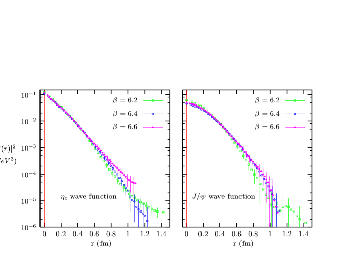
Figure 6: Scaling analysis of pseudoscalar (left) and vector (right) matter wave functions. The vertical scale is logarithmic.

As in Ref. [39], we have extracted gauge invariant wave functions from lattice 4-point functions:

$$|\Psi(\vec{r})|^{2} = \langle c\bar{c}|(\psi_{c}^{\dagger}\psi_{c})(0)(\psi_{\bar{c}}^{\dagger}\psi_{\bar{c}})(\vec{r})|c\bar{c}\rangle=$$ (7)

$${\cal N}\sum_{\vec{x}}\langle\ {\rm Tr} \{ S(\vec{0},0;\vec{x},t_{1})\ Q\ S(\vec{0},2t_{1};\vec{x},t_{1})^{\dagger}\Gamma\gamma_{5}$$

$$S(\vec{0},2t_{1};\vec{x}+\vec{r},t_{1})\ Q^{\dagger}\ S(\vec{0},0;\vec{x}+\vec{r},t_{1})^{\dagger}\gamma_{5}\Gamma^{\dagger}\}\ \rangle$$

$S$ is the quark propagator and $\Gamma=\{\gamma_{5},\gamma_{i}\}$ for $\{{\rm\!\!\ {}^{1}S_{0},\!\!\ ^{3}S_{1}}\}$. We have measured matter and charge wave functions by setting $Q=\{1,\gamma_{0}\}$ respectively [40]. ${\cal N}$ is a normalization constant fixed by imposing normalization 1 to the wave function.

Table 5: Parameters of the fit to Eq. (8) of the $\eta_{c}$ and $J/\psi$ matter wave function. We give both the direct values of the wave function at the origin $\Psi(0)$ and the values derived from the fit, $\hat{\Psi}(0)$, in GeV³. The parameter $\rho$ is given in fermi.

$\beta$	$|\Psi_{\eta_{c}}(0)|^{2}$	$|\hat{\Psi}_{\eta_{c}}(0)|^{2}$	$p_{\eta_{c}}$	$\rho_{\eta_{c}}$	$|\Psi_{J/\psi}(0)|^{2}$	$|\hat{\Psi}_{J/\psi}(0)|^{2}$	$p_{J/\psi}$	$\rho_{J/\psi}$
6.0	0.156(6)	0.153(6)	1.24 (2)	0.155(4)	0.093(4)	0.089(3)	1.46(3)	0.210(5)
6.2	0.124(7)	0.117(3)	1.24 (2)	0.172(4)	0.063(3)	0.060(1)	1.59(2)	0.255(2)
6.4	0.108(5)	0.100(2)	1.20 (2)	0.176(3)	0.045(3)	0.0445(3)	1.59(1)	0.283(1)
6.6	0.117(9)	0.112(2)	1.14 (1)	0.164(2)	0.049(3)	0.0500(5)	1.57(2)	0.273(2)

A comparison between pseudoscalar and vector matter wave functions using the non-perturbatively improved clover Dirac operator is presented in Fig. 6. We have binned the wave function in bins of size $a/2$. We include in the figure results for $\beta=6.2$, 6.4 and $\beta=6.6$ which show very good scaling within errors, up to possible, small, finite size effects for $\beta=6.6$ which will be discussed in the next section. The observed pattern corroborates qualitatively the predictions of the heavy-quark model: the value of the wave function at the origin increases for the pseudoscalar, decreases for the vector. Table 5 presents the results of the fit of matter wave functions ($Q$ equal 1 in Eq. (7)) to the following ansatz motivated by the heavy quark non-relativistic approximation and the form of variational wave functions in potential models:

$$|\Psi(r)|^{2}=|\hat{\Psi}(0)|^{2}\exp\Big{\{}-\Big{(}\frac{r}{\rho}\Big{)}^{p}\Big{\}}\,.$$ (8)

Our fits have been performed for $r\leq 0.8$ fm. In all cases we obtain a $\chi^{2}/ndf<0.5$ ($<$1.4 for $\beta=6.0$). In infinite volume, wave function normalization fixes the value of the wave function at the origin to $|\hat{\Psi}(0)|^{2}=p/(4\pi\rho^{3}\Gamma[\frac{3}{p}])$, a relation well satisfied by our fits. Given the good scaling properties of our $\beta=6.6$ and 6.4 wave functions one can extract an estimate of the continuum values of the pseudoscalar and vector wave functions at the origin. Fitting to a constant the results for these two values of $\beta$ we obtain $|\Psi_{\eta_{c}}(0)|^{2}=0.110(4)$ and $|\Psi_{J/\psi}(0)|^{2}=0.047(2)$. This quantity is of phenomenological interest since it enters in many of the estimates of the heavy quark approximation as well as in potential models for heavy quarks. One example, apart from the hyperfine splitting, is the leptonic decay width of the $J/\psi$ which, in the non-relativistic approximation, can be expressed as:

$$\Gamma(J/\psi\rightarrow e^{+}e^{-})=\frac{16\pi Q_{c}^{2}\alpha^{2}}{m^{2}_{J/\psi}}|\Psi(0)|^{2}$$ (9)

with $Q_{c}$ the charm quark charge in units of the proton charge and $\alpha$ the fine structure constant. Inserting our value of the $J/\psi$ wave function at the origin we obtain $\Gamma(J/\psi\rightarrow e^{+}e^{-})=5.8\pm 0.2$ keV, probably in too good agreement with the experimental value $\Gamma_{\rm exp}(J/\psi\rightarrow e^{+}e^{-})=5.26\pm 0.37$ keV, taking into account that formula (9) does not include radiative corrections (appart from those affecting the wave function) which, estimated to lowest order, multiply the right hand side of Eq. (9) by a factor $1-16\ \alpha_{s}(4m^{2}_{c})/(3\pi)\sim 0.5$ [35, 38].

We can also make use of formulas (5) and (6) to extract an estimate of the magnitude of non-perturbative contributions to the wave function at the origin ($\delta_{\rm NP}$). For this we use $m_{c}(m_{c})=1.301(34)$ GeV from [31] and extract from the equations both $\delta_{\rm NP}$ and $\alpha_{s}$. Plugging our values for $|\Psi_{\eta_{c}}(0)|^{2}$ and $|\Psi_{J/\psi}(0)|^{2}$ gives $\delta_{\rm NP}=-0.12$ and $\alpha_{s}=0.761$. The large value of $\alpha_{s}$ needed to match our results is a clear indication that spin dependent, and hence relativistic, non-perturbative effects are indeed rather strong for these charmonium states. If we would instead fix the strong coupling constant to $\alpha_{s}\sim 0.5$ as in [35] we would obtain a strong spin dependence of $\delta_{\rm NP}$ which would moreover turn out to be of ${\cal O}(1)$ for the $\eta_{c}$ wave function.

2.5 Finite volume effects

Table 6: Pseudoscalar mass and hyperfine splitting from non-perturbatively improved clover Dirac operator. The lattice spacing is fixed to 0.093 fm ($\beta=6.0$) and the number of lattice points $L$, hence the physical volume $La$, is varied as indicated in the table. Results, averaged over 100 configurations (190 for $L=8$), are given in physical units (MeV) with the scale set by $r_{0}$.

$L$	$La$ (fm)	$\!\!\ {}^{1}S_{0}$	$\!\!\ {}^{3}S_{1}$	$\!\!\ {}^{3}S_{1}-\!\!\ ^{1}S_{0}$
8	0.75	2958(10)	3019(12)	61.4(4.4)
10	0.93	2953(5)	3023(6)	70.6(2.5)
12	1.12	2957(3)	3032(5)	75.4(2.7)
14	1.30	2947(3)	3020(4)	72.6(1.9)
16	1.49	2952(3)	3025(4)	74.9(2.1)
18	1.68	2949(2)	3021(3)	72.5(1.5)

In this section we investigate how our results depend on the physical lattice volume. In particular we are interested in what happens with our finest $\beta=6.6$ lattice which has a somewhat small physical size $La=1.3$ fm. An indication of the magnitude of finite volume effects can already be obtained from the wave function plots and fits in the previous section. Compare in Fig. 6 the results for $\beta=6.6$ ($La$=1.3 fm) and $\beta=6.4$ ($La$=1.6 fm). Within errors, the wave functions do not show any clear signal of finite size effects, except for a small deviation of the pseudoscalar wave function at the tail, which is, however, not very significant within our errors. One could also argue from the fits in Table 5 that the wave functions at the origin are slightly larger than expected for the $La$=1.3 fm lattice, but this may be just a reflection, through the wave function normalization, of the finite volume effects at the tail. It is, anyway, clear from these plots that finite size effects on the charmonium wave function are really small on the $La$=1.3 fm lattice. In consequence, we do not expect the hyperfine splitting on this lattice to be significantly affected.

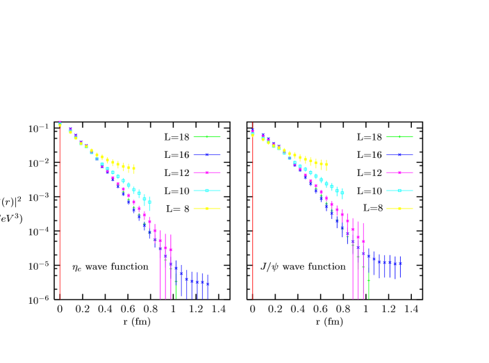
Figure 7: Finite volume effects on $\beta=6.0$ pseudoscalar (left) and vector (right) wave functions.

A complete finite volume analysis, including the volume dependence of the hyperfine splitting in the continuum limit, is beyond the scope of this paper. To address the question of the relevance of finite volume effects, we have decided to study instead a set of $L$= 8, 10, 12, 14, 16 and 18 lattices at the coarsest, $\beta=6.0$, lattice spacing. Table 6 presents our results for the pseudoscalar and vector masses and the hyperfine splitting for $\kappa=0.11925$, corresponding, for $L$=18, to a pseudoscalar mass of $M(\!\!\ ^{1}S_{0})=2949(2)$MeV. Our results are not precise enough to attempt a fit of the volume dependence. Still, the variation of the hyperfine splitting amounts to at most $4\%$ for $La>1$ fm. Further indication about the smallness of finite volume effects for lattices larger than 1 fm comes from the study of the volume dependence of wave functions. Fig. 7 shows the results for the set of lattices in Table 6. Deviations from the large volume behavior are negligible for $La>1.12$ fm.

3 Conclusions

Table 7 compiles our result for the $J/\psi-\eta_{c}$ hyperfine splitting together with previous determinations using other lattice formalisms [10, 6]. Our result is obtained with the non-perturbatively improved clover Dirac operator. The systematic error covers the difference between choosing as reference scale for charm the $\eta_{c}$ or $J/\psi$ mass as well as different continuum extrapolations (including or not $\beta=6.0$). Our final result is $\Delta M(J/\psi-\eta_{c})=77(2)(6){\rm MeV}$.

Table 7: Hyperfine splitting in MeV from different lattice approaches. The scale is set by $r_{0}$ or by the spin-averaged $\overline{P}\!-\!\overline{S}$ splitting. The result quoted as ‘This work’ is obtained from the non-perturbatively improved clover Dirac operator.

	This work	CP-PACS [10]	CP-PACS [10]	latest NRQCD[6]
Formalism	Relativistic	Relativistic	Relativistic	Non relativistic
Lattice	Isotropic	Anisotropic	Anisotropic
Extrapolation	Continuum	Continuum	Continuum
Scale	$r_{0}$	$r_{0}$	$\overline{P}-\overline{S}$	$\overline{P}-\overline{S}$
$\Delta M$	$77(2)(6)$	$72.6(9)^{(+1.2)}_{(-3.8)}$	$85.3(4.4)^{(+5.7)}_{(-2.5)}$	55(5)

Our value for the quenched hyperfine splitting within the OZI approximation remains 30$\%$ below the experimental result. Dynamical quark effects are usually expected to be ${\cal O}(10-20)\%$, which amounts for a large part but not all of the discrepancy. Actual dynamical quark effects may turn out to be larger for this particular quantity but the remaining discrepancy might also be due to the OZI approximation.

Our study shows the virtue of the “brute force” approach: reliable, consistent continuum extrapolations can be obtained from improved or non-improved discretizations if the lattice is fine enough. Conversely, using a coarse lattice implies continuum extrapolations where non-leading terms may be significant, thus introducing a systematic error which is very hard to control. From our study, the boundary between these two regimes sits where one would expect, around $aM_{q\bar{q}}\sim 1$.

Remarkably however, the non-perturbatively improved clover Dirac operator appears to give reliable extrapolations even starting from $aM_{q\bar{q}}\sim 1.4$. Non-leading terms remain small, perhaps because leading corrections ${\cal O}(a^{2})$ are themselves very small. We consider our Fig. 5 as a spectacular advertisement for using this Dirac discretization.

We believe our result finally closes the long debate on the magnitude of the quenched charmonium hyperfine splitting (within the OZI approximation). While NRQCD or an anisotropic discretization may yield a similar value, the reliability of such a result remains questionable: in the first case, one deals with an effective theory where the continuum limit cannot be taken; in the latter, the advantage over isotropic lattices in removing ${\cal O}(am_{q})^{n}$ scaling violations remains unclear. Until this point is settled, and although very accurate results can be obtained with anisotropic actions, this reduction in statistical errors can be more than offset by an increase in systematic errors due to possible scaling violations. Anisotropic lattices may be very useful in other contexts of course like for instance at finite temperature. Perhaps our result can be used to fine-tune the anisotropic actions involved.

Note finally that the charmonium system is ideally suited for a precision study on the current generation of PC clusters. Large, quenched lattices can be simulated efficiently with little inter-node communication, and high accuracy can be obtained at small cost. This computer environment seems well suited for a measurement of OZI-effects.

Acknowledgments

We thank Sara Collins for providing the raw UKQCD data and Stefan Sint for discussions and for pointing out the possible relevance of OZI suppressed diagrams. Numerical simulations have been performed on the SX5 at the Research Center for Nuclear Physics, Osaka University.

References

- [1]
- [2] W. E. Caswell and G. P. Lepage, Phys. Lett. B 167 (1986) 437. G. T. Bodwin, E. Braaten and G. P. Lepage, Phys. Rev. D 51 (1995) 1125 [Erratum-ibid. D 55 (1997) 5853] [arXiv:hep-ph/9407339].
- [3] A. Pineda and J. Soto, Nucl. Phys. Proc. Suppl. 64 (1998) 428 [arXiv:hep-ph/9707481].
- [4] M. E. Luke, A. V. Manohar and I. Z. Rothstein, Phys. Rev. D 61 (2000) 074025 [arXiv:hep-ph/9910209].
- [5] A. H. Hoang,“Heavy quarkonium dynamics”, In Shifman, N. (ed.) ‘At the frontier of particle physics’ Vol. 4, 2215-2331, World Scientific, Singapore [arXiv:hep-ph/0204299].
- [6] H. D. Trottier, Phys. Rev. D55 (1997) 6844 [arXiv:hep-lat/9611026]. N. H. Shakespeare and H. D. Trottier, Phys. Rev. D 58, 034502 (1998) [arXiv:hep-lat/9802038].
- [7] P. Boyle (UKQCD Collaboration), “The heavy quarkonium spectrum from quenched lattice QCD”, arXiv:hep-lat/9903017; Nucl. Phys. B (Proc. Suppl.) 63 (1998) 314 [arXiv:hep-lat/9710036].
- [8] T. R. Klassen,Nucl. Phys. B (Proc. Suppl.) 73 (1999) 918 [arXiv:hep-lat/9809174].
- [9] CP-PACS Collaboration (A. Ali Khan et al.), Nucl. Phys. B (Proc. Suppl.) 94 (2001) 325 [arXiv:hep-lat/0011005].
- [10] CP-PACS Collaboration (M. Okamoto et al.), Phys. Rev. D 65 (2002) 094508 [arXiv:hep-lat/0112020].
- [11] P. Chen, Phys. Rev. D64 (2001) 034509 [arXiv:hep-lat/0006019]. P. Chen, X. Liao and T. Manke, Nucl. Phys. B (Proc. Suppl.) 94 (2001) 342 [arXiv:hep-lat/0010069].
- [12] C. W. Bernard, Nucl. Phys. Proc. Suppl. 94, 159 (2001) [arXiv:hep-lat/0011064]. S. M. Ryan, Nucl. Phys. Proc. Suppl. 106, 86 (2002) [arXiv:hep-lat/0111010]. N. Yamada, arXiv:hep-lat/0210035.
- [13] C. McNeile, “Heavy quarks on the lattice,” arXiv:hep-lat/0210026.
- [14] A. X. El-Khadra, Nucl. Phys. Proc. Suppl. 30 (1993) 449 [arXiv:hep-lat/9211046]. A. X. El-Khadra, G. Hockney, A. S. Kronfeld and P. B. Mackenzie, Phys. Rev. Lett. 69 (1992) 729.
- [15] C. Stewart and R. Koniuk, Phys. Rev. D63 (2001) 054503 [arXiv:hep-lat/0005024].
- [16] A. X. El-Khadra, S. Gottlieb, A. S. Kronfeld, P. B. Mackenzie and J. N. Simone, Nucl. Phys. Proc. Suppl. 83 (2000) 283. M. Di Pierro et al., “Charmonium with three flavors of dynamical quarks,” arXiv:hep-lat/0210051.
- [17] F. Karsch, Nucl. Phys. B 205 (1982) 285. G. Burgers, F. Karsch, A. Nakamura and I. O. Stamatescu, Nucl. Phys. B 304 (1988) 587.
- [18] J. Harada, A. S. Kronfeld, H. Matsufuru, N. Nakajima and T. Onogi, Phys. Rev. D 64 (2001) 074501 [arXiv:hep-lat/0103026].
- [19] S. Aoki, Y. Kuramashi, and S. i. Tominaga, “Relativistic heavy quarks on the lattice”, Prog. Theor. Phys. 109 (2003) 383 [arXiv:hep-lat/0107009]; Nucl. Phys. Proc. Suppl. 106 (2002) 349 [arXiv:hep-lat/0111025].
- [20] T. Umeda, R. Katayama, O. Miyamura, H. Matsufuru, Int. J. Mod. Phys. A 16 (2001) 2215.
- [21] J. Harada, H. Matsufuru, T. Onogi and A. Sugita, Phys. Rev. D 66 (2002) 014509 [arXiv:hep-lat/0203025].
- [22] S. Choe et al. [QCD-TARO Collaboration], Nucl. Phys. Proc. Suppl. 106 (2002) 361 [arXiv:hep-lat/0110104].
- [23] C. McNeile, C. Michael and K. J. Sharkey [UKQCD Collaboration], Phys. Rev. D 65, 014508 (2002) [arXiv:hep-lat/0107003].
- [24] T. Struckmann et al. [TXL Collaboration], Phys. Rev. D 63, 074503 (2001) [arXiv:hep-lat/0010005].
- [25] A. De Rújula, H. Georgi and S. L. Glashow, Phys. Rev. D 12 (1975) 147.
- [26] N. Isgur, Phys. Rev. D12 (1975) 3770-3774; ibid. 13 (1976) 122-124.
- [27] C. McNeile and C. Michael [UKQCD Collaboration], Phys. Rev. D 63, 114503 (2001) [arXiv:hep-lat/0010019].
- [28] S. Necco and R. Sommer, Nucl. Phys. B 622 (2002) 328 [arXiv:hep-lat/0108008]. S. Necco, “The static quark potential and scaling behavior of SU(3) lattice Yang-Mills theory,” arXiv:hep-lat/0306005.
- [29] M. Lüscher et al., Nucl. Phys. B491 (1997) 323 [arXiv:hep-lat/9609035].
- [30] S. Collins, PhD thesis, The University of Edinburgh (1993).
- [31] J. Rolf and S. Sint, Nucl. Phys. Proc. Suppl. 106 (2002) 239 [arXiv:hep-ph/0110139]. J. Rolf and S. Sint [ALPHA Collaboration], JHEP 0212 (2002) 007 [arXiv:hep-ph/0209255].
- [32] UKQCD Collaboration (K. C. Bowler et al.). Nucl. Phys. B 619 (2001) 507 [arXiv:hep-lat/0007020].
- [33] A. X. El-Khadra, A. S. Kronfeld and P. B. Mackenzie, Phys. Rev. D 55 (1997) 3933 [arXiv:hep-lat/9604004].
- [34] N. Isgur and H. B. Thacker, Phys. Rev. D 64 (2001) 094507 [arXiv:hep-lat/0005006].
- [35] F. J. Yndurain, “The theory of Quark and Gluon interactions”, Springer-Verlag, Berlin Heidelberg 1993.
- [36] S. Titard and F. J. Yndurain, Phys. Rev. D 51, 6348 (1995) [arXiv:hep-ph/9403400]; Phys. Rev. D 49, 6007 (1994) [arXiv:hep-ph/9310236].
- [37] H. Leutwyler, Phys. Lett. B 98, 447 (1981). M. B. Voloshin, Sov. J. Nucl. Phys. 36, 143 (1982) [Yad. Fiz. 36, 247 (1982)].
- [38] R. Barbieri, R. Gatto, R. Kogerler and Z. Kunszt, Phys. Lett. B 57, 455 (1975). R. Barbieri, E. d’Emilio, G. Curci and E. Remiddi, Nucl. Phys. B 154, 535 (1979).
- [39] C. Alexandrou, P. de Forcrand and A. Tsapalis, Phys. Rev. D 66, 094503 (2002) [arXiv:hep-lat/0206026].
- [40] A. M. Green, J. Koponen, P. Pennanen and C. Michael [UKQCD Collaboration], Phys. Rev. D 65, 014512 (2002) [arXiv:hep-lat/0105027]; “Radial correlations between two quarks,” arXiv:hep-lat/0106020.