Lattice Results on the Connected Neutron Charge Radius

Abstract

We describe a calculation using quenched lattice QCD of the connected part of the neutron electric form factor for momentum transfers in the range $0.3\,{\rm GeV^{2}}\stackrel{{\scriptstyle<}}{{\sim}}-q^{2}\stackrel{{\scriptstyle<}}{{\sim}}1.0\,{\rm GeV^{2}}$. We extract the implied charge radius using a Galster parameterization and consider various ways of extrapolating the neutron charge radius value to the chiral limit. We find that the measured charge radii may be reconciled to experiment by standard phenomenology and lowest or next to lowest order contributions from chiral perturbation theory.

I Introduction

There has been a surge of interest and activity in evaluating electromagnetic form factors of nucleons, both on the experimental exp and theoretical (lattice) side the . Unfortunately, knowledge of the neutron electric form factor, $G^{n}_{e}(q^{2})$, has lagged behind. The extraction of this fundamental quantity is difficult because of the dominance of the magnetic contribution in unpolarized measurements. In addition, free neutron targets do not exist making its measurement from deuteron targets prone to model dependent systematic errors of the order of $\sim 30\%$ bermuth . However, new types of experiments with a polarized electron beam and deuteron or ³He targets now lead to measurements of $G^{n}_{e}(q^{2})$ with greatly improved accuracy gao ; bermuth .

There are reasons to believe that this form factor is the most interesting and revealing of the four nucleon electromagnetic form factors. The contribution of the various flavored sea and cloud quark components will no longer be hidden behind a huge valence contribution, as is the case for the other electromagnetic form factors, and the sizes of the non-valence components could hold some surprises. Lattice QCD was invented to reliably sort out such subtle effects, and it will be a major accomplishment to predict/explain these properties.

The calculation described here is of the “connected” part of $G^{n}_{e}(q^{2})$. The electromagnetic current is a sum of the charge-weighted flavor currents, each of which is a color singlet. Thus there are also quark self-contraction graphs, usually called “disconnected” graphs, involving the various flavor currents which can also contribute to this quantity. (These self-contraction loops are of course connected to the valence or cloud quarks by gluons.) We do not attempt to calculate these graphs, but will comment on the significance of our results for the disconnected contribution in Section V.

Previous lattice calculations of nucleon electromagnetic form factors using Wilson one ; two ; three and improved fermions the have had good signals for the proton electric and magnetic form factors, $G^{p}_{e}(q^{2})$ and $G^{p}_{m}(q^{2})$, as well as the neutron magnetic form factor, $G^{n}_{m}(q^{2})$, but noisy results for the neutron electric form factor, $G^{n}_{e}(q^{2})$. Similar to experiment, the lattice extraction of this form factor is the most difficult. If lattice studies are to keep pace with the improved experiments referenced above, we must move beyond the qualitative stage in the calculation of this physical quantity. A new, more precise, lattice calculation of $G^{n}_{e}(q^{2})$ is described here. The lattice used is larger ($20^{3}\times 32$), more configurations ($100$) are employed than in Ref. one , and more sophisticated analysis methods are used.

Although we will calculate the electric form factor at several nonzero momentum transfers, we prefer at this point to concentrate on the implied charge radius, a zero momentum quantity which should allow a more reliable chiral extrapolation. We will see that the neutron charge radius is a useful laboratory in which the physics of the quenched approximation can be studied, and its shortcomings quantified. One of the effects of quenching on our results comes through the double pole “hairpin” graphs. We will consider these graphs separately and provisionally conclude that these do not have a significant effect on our extrapolations. We think it extremely likely that the quenched approximation gives a good representation of the connected part of $G^{p}_{e}(q^{2})$. The quenched, connected simulations quoted above have yielded phenomenologically acceptable chirally extrapolated electromagnetic form factors for both mesons and baryons. The quenched approximation has also been generally successful in evaluating other quantities such as, for example, scalar and axial nucleon form factors others . The validity of this approximation, however, can not be assured and subtle dynamical/disconnected effects may remain. We will suggest further investigations which should help form a more complete physical picture in Section V.

II Numerical Details

The periodic gauge configurations used in this study were generated from the standard one-plaquette action at $\beta=6.0$ on $20^{3}\times 30$ lattices. These lattices were slightly enlarged to $20^{3}\times 32$ by copying each time edge to the opposite side because of an inverter requirement that at least one of the dimensions be an integral multiple of 8 wliu . The Cabibbo-Marinari pseudo heatbath was used and configurations were separated by at least 1000 sweeps. No significant auto correlations were observed in the real or imaginary parts of the nucleon correlators. 100 configurations were used in the charge radius analysis.

We used $\kappa=0.150,0.152,0.153,$ and $0.154$ in the standard Wilson quark action. The pion masses used are

$m_{\pi}a=0.578(2),\,\,0.4772^{+9}_{-2}$ iwasaki ,   $0.4237(8)$ gock ,    $0.364(1)$ allton

respectively. The nucleon masses, previously reported in Ref. randy on 2000 configurations, are

$m_{N}a=0.997(7),\,\,0.869(2),\,\,0.799(2),\,\,0.728(3)$

(The pion and nucleon masses at $\kappa=0.150$ were measured here on $t$=15 to 18 single exponential fits, where t=0 is the time origin of the quark propagators.) The lattice spacing is taken to be the same as in Ref. randy ,

a = 0.1011(7) fm

obtained in Ref. gock from the physical string tension. The authors of Ref. three used the physical nucleon mass instead to arrive at $a=0.115(6)$fm.

The electric form factors were measured from point source neutron two and three point functions with the ratio given in Ref. one , with zero and non-zero momentum two point functions evaluated at timestep $t^{\prime}=9$:

$$G_{e}(q^{2})=\left(\frac{2E}{E+m}\right)^{1-\frac{t_{1}}{t^{\prime}}}\left(\frac{G_{nJ_{4}n}(t_{2},t_{1};0,-\vec{q},\Gamma_{4})}{G_{nn}(t_{2};0,\Gamma_{4})}\right)\left(\frac{G_{nn}(t^{\prime};0,\Gamma_{4})}{G_{nn}(t^{\prime};\vec{q},\Gamma_{4})}\right)^{\frac{t_{1}}{t^{\prime}}}.$$ (1)

The time ordered two point function, using the standard neutron interpolation field, $\chi_{\alpha}^{n}(x)=\epsilon^{abc}\psi_{\alpha}^{(d)a}(x)\psi_{\beta}^{(d)b}(x)(\tilde{C})_{\beta\gamma}\psi_{\gamma}^{(u)c}(x)$, where $\tilde{C}=C\gamma_{5}$ and $C$ is the charge conjugation matrix, is (understood $\alpha$, $\alpha^{\prime}$ sums)

$$G_{nn}(t;\vec{p},\Gamma)\equiv\displaystyle{\sum_{\vec{x}}}e^{-i\vec{p}\cdot\vec{x}}\Gamma_{\alpha^{\prime}\alpha}\langle{\rm vac}|T\left(\chi_{\alpha}^{n}(x)\overline{\chi}_{\alpha^{\prime}}^{n}(0)\right)|{\rm vac}\rangle,$$ (2)

where $\Gamma_{4}\equiv\frac{1}{2}\left(\begin{array}[]{cc}I&~{}~{}~{}~{}0\\ 0&~{}~{}~{}~{}0\end{array}\right)$ in the $4\times 4$ Dirac space. The three point function we need, which uses the lattice conserved vector current, $J_{\mu}(x)$, is ($\vec{q}=\vec{p}-\vec{p}^{\prime}$)

$$G_{nJ_{\mu}n}(t_{2},t_{1};\vec{p},{\vec{p}\,^{\prime}},\Gamma)\equiv-i\displaystyle{\sum_{\vec{x}_{2},\vec{x}_{1}}}e^{-i\vec{p}\cdot\vec{x}_{2}}e^{i\vec{q}\cdot\vec{x}_{1}}\Gamma_{\alpha^{\prime}\alpha}\langle{\rm vac}|T\left(\chi_{\alpha}^{n}(x_{2})J_{\mu}(x_{1})\overline{\chi}_{\alpha^{\prime}}^{n}(0)\right)|{\rm vac}\rangle.$$ (3)

The time position of the conserved charge density operator, $J_{4}(x_{1})$, which is extended one lattice link in the time direction, is associated with the midpoint of that link, which means half-integer values for $t_{1}$.

III results

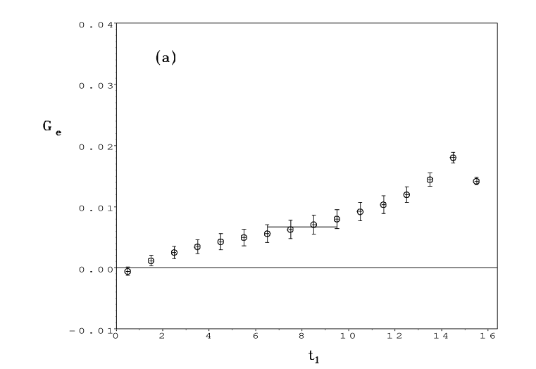
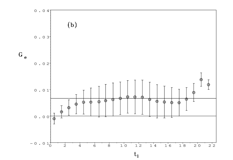
Figure 1: (a) $\kappa=0.152$ electric form factor data for $p=\pi/10$ on the source separation $\Delta t=15$ lattice for 100 configurations. (b) Similar graph on the source separation $\Delta t=21$ lattice for 50 configurations. The fit value on the $\Delta t=15$ data is shown superimposed on the $\Delta t=21$ data in the (b) part.

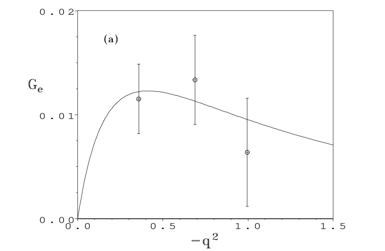
Figure 2: (a) $\kappa=0.154$ neutron electric form factor data compared to the Galster fit as a function of $-q^{2}$ in GeV². (b) Similar graph for $\kappa=0.153$.

In Figs.1(a) and (b) we show an example of the raw data fits, in this case for $\kappa=0.152$ and the lowest momentum transfer, where the time axis represents $t_{1}$ in Eq.(1). In order to establish reliable source positions for maintaining a good signal, we originally did the calculations on 50 configurations with point nucleon sources at time steps 6 and 27. This is the $\Delta t=21$ data referred to in Fig.1(b). The (b) part of the figure shows that a good plateau is already forming at time step 7, although error bars are large. This allowed us to move the final source position to time location 21, giving $\Delta t=15$ between sources, and three point correlation data at time steps 7 - 10 relative to the origin were fit. The lowest three momentum transfers had similar plateaus and form factor values were extracted for the other $\kappa$ values. Fig.2 illustrates the form factors found at $\kappa=0.154$ and $0.153$; numerical values and error bars are given in Table I. The error bars on the form factors only appear relatively large because of the small central values. Comparing results at $\kappa=0.154$, the error bars here are a factor of approximately 5 times smaller than the similar calculation in Ref. one . (They are also significantly smaller than error bars given in Ref. three , although individual ${\kappa}$ results are not given.) With the adopted scale for $a$, our smallest four-momentum transfer range on these measurements is about $0.3{\rm GeV^{2}}$, about half that used in Ref. one .

Before we go on to the charge radius fits, let us explain some of the philosophy of our fits of the electric form factor data. A well known phenomenological form for $G^{n}_{e}(q^{2})$ is the Galster parameterization galster ,

$$G^{gal}_{e}(q^{2})=-\frac{\tau\mu}{1+p\tau}G^{D}(q^{2}),$$ (4)

where $\tau\equiv-q^{2}/4m_{N}^{2}$, where $m_{N}$ is the nucleon mass and

$$G^{D}(q^{2})=\frac{1}{(1-\frac{q^{2}}{m_{D}^{2}})^{2}},$$ (5)

is the dipole form factor using the dipole mass, $m_{D}$. The most often used value of the parameter $p$ is 5.6 and $\mu\sim-1.91$ is the neutron magnetic moment. The neutron squared charge radius, given by

$$r^{2}_{n}=6\frac{dG^{n}_{e}(q^{2})}{dq^{2}}|_{q^{2}=0},$$ (6)

implied by the Galster form is $r^{2}_{n}=3\mu/2m_{N}^{2}=-3.24$ GeV^-2, which is only about $9\%$ different from the experimental value, $r^{2}_{n}=-2.982(6)$ GeV^-2 rpp . This form is used to fit the form factor data given in Table I. At each value of $\kappa$ we have three values of $G_{e}^{n}(q^{2})$. There are also three parameters in the Galster form: $p$, $\mu$, and $m_{D}$. It is essential to have at least one degree of freedom in the fits so that error bars and $\chi^{2}$ goodness of fits can be defined. Dipole masses for Wilson fermion fits of the proton electric form factor were given in Table VII of Ref. one at $\kappa=0.154$ and $0.152$. These values are adopted as input and listed in GeV in Table II, along with the nucleon masses given above. In addition, the values at $\kappa=0.153$ and $0.150$ were interpolated from the $\kappa=0.154,0.152,0.150$ dipole masses given in Ref. one . These were plotted as a function of dimensionless quark mass, defined as $\ln(4\kappa_{c}/3\kappa-3)$, where we used the central value in $\kappa_{c}=0.157096(28)^{+33}_{-9}$ iwasaki . A linear plus constant fit produced an excellent interpolation with $\chi^{2}=0.025$. The final Galster parameters for the four fits are listed in Table II and are shown in Fig.2. Again, the error bars on the extracted -$r^{2}_{n}$ appear large, but even at the largest $\kappa$ the error bar is about 6 times smaller than the experimental value for this quantity. The error bars could have been made significantly smaller by fixing the $p$ value in the Galster fits, but we choose not to do this.

In our chiral fits we are extrapolating the neutron charge radius using the formulas in the Appendix from heavy baryon chiral perturbation theory and parameters in Table III across our four $m_{\pi}^{2}$ values to the physical charged pion mass at $139$ MeV. In doing these extrapolations, it is necessary to adopt values of $f_{\pi}$ and $\Delta$ (the octet-decuplet mass difference). Our point of view is that we are extrapolating down toward the chiral limit from our lowest pion mass at $\kappa=0.154$, so our values of $f_{\pi}$ and $\Delta$ are measured at this value down . With our value of $a^{-1}$, the result of Table 4 of Ref. allton gives $\Delta=158$ MeV, and Table VIII of Ref. me2 gives $f_{\pi}=120$ MeV at $\kappa=0.154$ when the $a^{-1}$ value adopted here is supplied. (It is also consistent with the interpolated $f^{PT}_{\pi}$ value at $\kappa=0.154$ from Table XX of Ref. iwasaki .) We also adopt the tree level QCD values $D=0.8$ flores , the axial vector octet-octet coupling, and $|{\cal C}|=1.4$ butler , the axial vector octet-decuplet coupling. These last two quantities are fixed from phenomenology at the chiral limit, so we can not claim complete consistency point . Of course, other extrapolation schemes can be used, and the first reference in the for example assumes some parameter values at the chiral limit and extrapolates upward in $m_{\pi}^{2}$ toward their measured (isovector) charge radii and magnetic moments using other parameters.

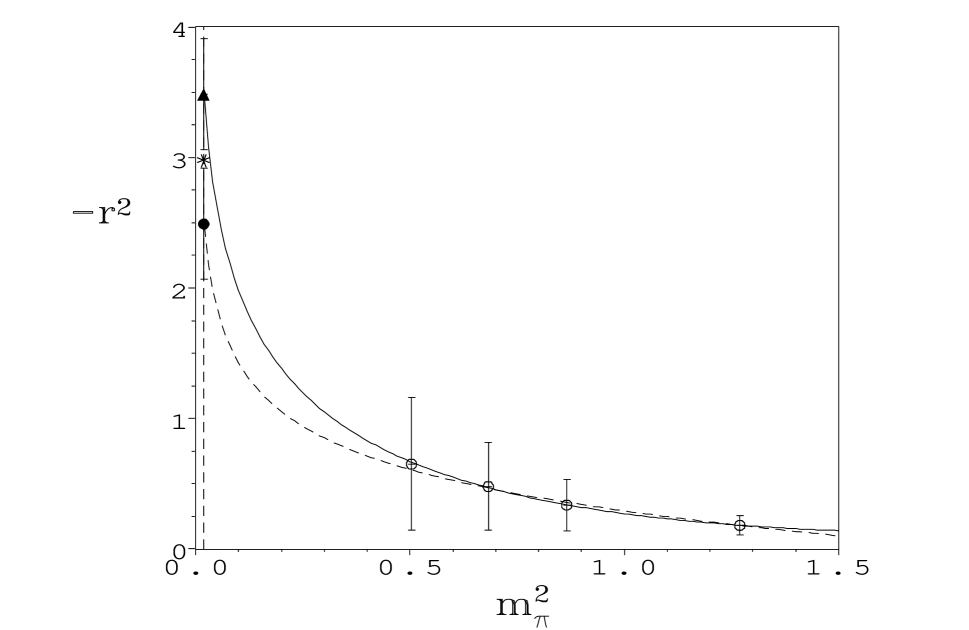
Figure 3: Two chiral extrapolations of the neutron charge radius data (in ${\rm GeV}^{-2}$) as a function of pion mass squared (in ${\rm GeV^{2}}$). The solid line is the pure quenched octet (“O” in Table IV) extrapolation, the dashed line gives the octet plus decuplet (“O+D”). The vertical dashed line represents the physical pion mass squared and the burst on this line represents the experimental charge radius. The lattice data are represented by open circles and are given as a function of squared pion mass in ${\rm GeV^{2}}$. Error bars are given on the extrapolated values (triangle - octet, solid circle - octet plus decuplet) at the physical pion mass squared.

Fig.3 shows two extrapolations of the -$r^{2}_{n}$ values as a function of $m_{\pi}^{2}$ using these parameters. One curve in Fig.3 assumes only quenched octet intermediate states, labelled “O” in Table IV. ($C_{1}$, $C_{2}$ give the analytic contribution to -$r^{2}_{n}$ and are defined in the Appendix.) Perhaps surprisingly this produces an excellent fit of the data. Although the charge radii values are initially small, they extrapolate to a physical charge radius which is consistent within errors with the measured experimental result because of the chiral logs. The other curve in Fig.3, the “O+D” result from Table IV, gives the result for adding the leading octet and decuplet contributions. As one can see this lowers the extrapolated -$r_{n}^{2}$, which is still consistent with experiment. The error bars on the charge radius values at the chiral limit come almost completely from the uncertainty in the $C_{1}$ values from Table IV, since the physical pion mass is essentially at the chiral limit. The uncertainties in $C_{1}$ and $C_{2}$ (given by $\pm 0.43$ GeV^-2 and $\pm 0.35$ GeV^-4, respectively) are independent of the fit (as is the uncertainty in the extrapolated -$r_{n}^{2}$, as listed in the Table) since in the Marquardt algorithm of Ref. marq the uncertainties are determined by either analytical or numerical derivatives of the functional form with respect to the adjustable parameters. Since these are just constant plus linear fits in $m_{\pi}^{2}$, the fixed nonanalytic part does not affect the uncertainties in $C_{1}$, $C_{2}$ or the extrapolated -$r_{n}^{2}$.

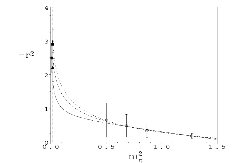
Figure 4: Three chiral extrapolations of the neutron charge radius data (in ${\rm GeV}^{-2}$) as a function of pion mass squared (in ${\rm GeV^{2}}$). From top to bottom (shortest dashed line to longest). All fits take into account both the octet and decuplet. The top line gives the result of the higher order fit (“(O+D)(h)” in Table IV), the middle is the (lowest order) octet plus decuplet (“O+D”) also shown in Fig.3, and the lowest dashed line is the cutoff form (“(O+D)(c)”). The solid square, circle and triangle give the chiral values of these three fits, respectively. The solid circle has been moved to the left for clarity of observations of the various error bars. See Fig. 3 for meanings of the other symbols.

Fig.4 contrasts the “O+D” fit found in Fig.3 with two changed forms which also involve both the octet and decuplet. One of these is the “cutoff” form suggested in Ref. detmold in the context of parton distribution functions, labelled as “(O+D)(c)” in Table IV. The other form is the higher order (in $1/m_{heavy}$) nonanalytic calculation of Ref. puglia , adapted to this quenched situation and labelled “(O+D)(h)” in Table IV. The figure illustrates that these forms can lower the extrapolated -$r_{n}^{2}$ and can have a significant impact ($\sim 10-30\%$) upon the chiral limit, which we think is a reasonable estimate of the systematic extrapolation error involved. The “(O+D)(h)” extrapolation raises the value from the “(O+D)” fit and essentially hits the experimental value exactly with a lowered $\chi^{2}_{r}$. It would be wrong to make too much of this agreement, but clearly the fits we are making are consistent with the lattice data and the experimental value for the neutron squared charge radius.

IV Hairpin Considerations

We have considered the quenched QCD contributions to the neutron and proton charge radius from the so-called hairpin graphs using the methods of labrenz . The leading nonanalytic parts of these diagrams are proportional to $\delta\ln({m_{\pi}^{2}/\mu^{2}})$ where $\delta\equiv m_{0}^{2}/(48\pi^{2}f_{\pi}^{2})$ (for $m_{u}=m_{d}$) and $m_{0}$ is the usual hairpin “mass” parameter. These diagrams are the direct analog of the magnetic hairpin graphs considered recently in Ref. savage . (See Figs. 2(a) and (b) of this reference for the relevant diagrams. The $\alpha_{\phi}$ interaction should not contribute to a leading log for magnetic moments or charge radii because of the two extra derivatives in the coupling.) Remarkably, we find that the contributions from these graphs vanish identically for the proton and neutron. There are three sets of such graphs plus wavefunction renormalization. The first set consists of a hairpin correction of the tree-level octet charge radius vertex. When this is combined with the wavefunction renormalization, these two contributions cancel identically, not only for the proton and neutron, but also for the other octet baryons comment . In addition, there is a contribution at this order to the charge radius from the electric quadrupole operator bss . It connects octet and decuplet baryon lines similarly to the transition magnetic moment operator in Ref. savage . It vanishes for the proton and neutron (although not for the other octet baryons) for the same reason that the magnetic transition operator does; namely, that the flavor-charge coefficient vanishes. In addition, there are one-loop hairpin contributions from the tree-level decuplet vertex, which also includes a wavefunction renormalization part. These do not cancel, but vanish separately for the proton and neutron, again because of the flavor-charge factor decuplet .

Unfortunately, there are also two-loop graphs which contribute at the same order as the one loop graphs within chiral perturbation theory. This can be understood simply from the physical dimensions of the charge radius, which goes like (mass)^-2. To lowest order in the hairpin interaction the modification of the tree-level charge radius is of order $\delta(r^{2}_{n})_{tree}$. However, a term of the same order with the usual chiral perturbation theory factor $1/(4\pi f_{\pi})^{2}$ replacing the factor of $(r^{2}_{n})_{tree}$ may also be generated from a two-loop graph involving a primitive electromagnetic interaction. Two-loop graphs have been considered recently in the context of mass corrections in Ref. mcgovern . These graphs are clearly related to the graphs we need since one of the pion loops may be changed to a hairpin loop just by differentiation with respect to the pion mass and changing the flavor factor. Although we have stopped short of their evaluation we can conclude from power counting that these charge radius graphs are logarithmically divergent in the loop momentum and can in principle contribute to the chiral log charge radius coefficient.

An estimate shows that the contribution of any such hairpin chiral logs in the proton and neutron charge radii should be small. Recently, there have been estimates of the value of $\delta$, the hairpin coefficient, from lattice simulations deltas . For concreteness we will take $\delta=0.2$. As an example of the expected magnitude of the effect of the delta interaction on the chiral log coefficient, let us take the magnitude of the ratio of the wavefunction renormalization contribution (canceled by the modified tree-level piece) to the quenched chiral coefficient for the proton or neutron:

$$R\equiv(\delta(r^{2}_{n})_{tree}(D-F)^{2})/(\frac{1}{(4\pi f_{\pi})^{2}}\frac{10}{3}D^{2}).$$ (7)

Our fits below (see the $C_{1}$ coefficients in Table IV) give $(r^{2}_{n})_{tree}<1$ GeV², so that for $D=0.8$, $F=0.5$ flores , we obtain at most $R\sim 0.05$. If we replace the $(r^{2}_{n})_{tree}$ by another factor of $1/(4\pi f_{\pi})^{2}$, which would happen at two loops, we get the same estimate. Of course, the flavor-charge coefficient here is specific to this interaction. However, barring an exceptionally large coefficient it is likely that the effect of hairpins on the chiral extrapolations will be negligible.

V Significance of Results

We have seen that one can come remarkably close to understanding the value of the neutron charge radius using quenched lattice QCD. Our calculations use the Wilson action and therefore are limited to rather large pion masses. Although standard values for the $D$ and $\mathcal{C}$ coefficients were used in the analysis, there is nothing to force the quenched values of these coefficients to be the same as in the full theory. The values we used should be considered merely typical, based on standard phenomenology. However, our results for -$r^{2}_{n}$ are consistent with the expected rise from the quenched chiral logs using these coefficients, and the fits to the data are excellent. Of course lattice calculations, both quenched and dynamical, probing further into the chiral limit would be helpful to verify this scenario.

We find that the higher order nonanalytic contributions in Ref. puglia or the possible “cutoff” form suggested in Ref. detmold can make a small but significant impact on the chiral extrapolations. According to the argument in Section IV, we do not expect hairpin contributions to make a significant contribution to the chiral log terms. However, we can not rule out the possibility of large coefficients entering and this remains a slim possibility. An exact evaluation of this quantity would be very welcome.

Of course, the disconnected part, which consists of up, down and strange quark loops, should be added to our results before we compare to experiment. Ref. three gives results for combined u, d, and s quarks and finds an increase of perhaps 0.5-1.0 GeV${}^{-2}\approx.019-039$ fm² in $-r_{n}^{2}$. (We are using the smallest $-q^{2}$ result from Fig.5(b) of this paper and the Galster parameterization.) The question naturally arises as to whether our results are compatible with such values. The fact that one finds good agreement with experiment using standard phenomenology and only the connected part of the amplitude argues that the disconnected contribution must be relatively small, again assuming the hairpin contribution is minor. An increase by the amount suggested in Ref. three could perhaps be accommodated by our data, but likely at the expense of the excellent fits found here. The present results illustrate the importance of establishing a reliable set of extrapolation parameters, which can only be done by extending lattice calculations for a variety of quantities closer to the chiral limit. For now, we conclude from our lattice study that the connected part of the quenched amplitude is capable of explaining the bulk of the neutron electric charge radius.

Note added: An independent discussion of charge radii in quenched and partially quenched ChPT has just appeared arndt .

VI Acknowledgements

This paper has had a prolonged gestation period and represents the final outcome of the preliminary results reported in Ref. me . A number of computer systems at the National Center for Supercomputing Applications were employed, including the CM2, CM5, Exemplar, Power Challenge, and Origin 2000 computers. The production runs on the CM5 utilized the fast conjugate gradient written by Weiqiang Liu wliu . The project was suggested to WW by Franz Gross and has been contributed to by Stephen Naehr, Phillip Kalmanson, and Nooman Karim under the Baylor University Research Experiences for Undergraduates Program. AT was supported by the Baylor University Postdoctoral Program. WW thanks Michael Ramsey-Musolf and K. F. Liu for helpful conversations and communications. It has been supported under NSF grants PHY-9203306, 9401068, 9722073, and 0070836 and in part by the Natural Sciences and Engineering Research Council of Canada. The Baylor University Sabbatical program is also gratefully acknowledged.

Appendix A: Quenched Chiral Charge Radii Expressions

We use the $f_{\pi}\approx 93{\rm MeV}$ normalization. For completeness we give the lowest order chiral expressions for both octet baryon charge radii as well as magnetic moments. The charge-flavor factors, $b^{(X)}_{N}$, are listed in Table III.

$$(\delta\mu)_{B}=\frac{m_{N}}{(4\pi f_{\pi})^{2}}\left(-\frac{\pi}{2}\sum_{X=\pi,K}b^{(X)}_{B}m_{X}\right)$$ (8)

$$(\delta r^{2})_{B}=\frac{1}{(4\pi f_{\pi})^{2}}\sum_{X=\pi,K}b^{(X)}_{B}\left(-{5\over 8}\ln\left(\frac{m_{X}^{2}}{\mu^{2}}\right)-\frac{7}{8}\right)$$ (9)

$$(\delta\mu)_{T}=\frac{m_{N}}{(4\pi f_{\pi})^{2}}\sum_{X=\pi,K}b^{(X)}_{T}\left(\frac{2}{3}\,F_{m}(m_{X},\Delta,\mu)+\frac{10\Delta}{9}\right)$$ (10)

$$F_{m}(m_{X},\Delta,\mu)\equiv\left\{\begin{array}[]{ll}-\Delta\ln\left(\frac{m_{X}^{2}}{\mu^{2}}\right)+2\sqrt{m_{X}^{2}-\Delta^{2}}\cos^{-1}\left(\frac{\Delta}{m_{X}}\right)&\mbox{,\,\,$m_{X}>\Delta$}\\ -\Delta\ln\left(\frac{m_{X}^{2}}{\mu^{2}}\right)-2\sqrt{\Delta^{2}-m_{X}^{2}}\ln(\frac{\Delta+\sqrt{\Delta^{2}-m_{X}^{2}}}{m_{X}})&\mbox{,\,\,$\Delta>m_{X}$}\end{array}\right.$$ (11)

$$(\delta r^{2})_{T}=\frac{1}{(4\pi f_{\pi})^{2}}\sum_{X=\pi,K}b^{(X)}_{T}\left(-\frac{5}{3}F_{r}(m_{X},\Delta,\mu)-\frac{26}{9}\right)$$ (12)

$$F_{r}(m_{X},\Delta,\mu)\equiv\left\{\begin{array}[]{ll}\ln\left(\frac{m_{X}^{2}}{\mu^{2}}\right)+\frac{2\Delta}{\sqrt{m_{X}^{2}-\Delta^{2}}}\cos^{-1}\left(\frac{\Delta}{m_{X}}\right)&\mbox{,\,\,$m_{X}>\Delta$}\\ \ln\left(\frac{m_{X}^{2}}{\mu^{2}}\right)+\frac{2\Delta}{\sqrt{\Delta^{2}-m_{X}^{2}}}\ln(\frac{\Delta+\sqrt{\Delta^{2}-m_{X}^{2}}}{m_{X}})&\mbox{,\,\,$\Delta>m_{X}$}\end{array}\right.$$ (13)

Note the sign typo in Eq.(6) of Ref. puglia in the $\Delta>m_{X}$ branch of $F_{r}(m_{X},\Delta,\mu)$. Although these quenched expressions do not appear in the literature, it is clear that they are implied by the results in Ref. kubis for the full QCD charge radii and the results of Ref. savage for the quenched magnetic moments since one can simply take the ratio of the quenched to full QCD coefficients in Table III of Ref. savage , and apply them to the full QCD charge radii results in kubis . (One must also drop the $D$, $F$ independent terms from Table 1 of kubis .) We have also independently verified the above results for charge radii and magnetic moments. We have left analytic parts in the expressions so that others may independently verify these results using dimensional regularization.

The functional form of the nonanalytic expressions used in the chiral extrapolations of the neutron $-r^{2}_{n}$ are given below.
Octet only:

$${\rm O}=-\frac{1}{(4\pi f_{\pi})^{2}}{10\over 3}D^{2}\ln\left(\frac{m_{\pi}^{2}}{\mu^{2}}\right).$$ (14)

Octet plus decuplet:

$${\rm O+D}=\frac{1}{(4\pi f_{\pi})^{2}}\left\{-{10\over 3}D^{2}\ln\left(\frac{m_{\pi}^{2}}{\mu^{2}}\right)+\frac{5}{6}{\cal C}^{2}F_{r}(m_{\pi},\Delta,\mu)\right\}.$$ (15)

Octet plus decuplet cutoff form:

$${\rm(O+D)(c)}={\rm O+D}+\frac{1}{(4\pi f_{\pi})^{2}}\left\{{10\over 3}D^{2}\ln\left(\frac{\Lambda^{2}+m_{\pi}^{2}}{\mu^{2}}\right)-\frac{5}{6}{\cal C}^{2}F_{r}(\sqrt{m_{\pi}^{2}+\Lambda^{2}},\Delta,\mu)\right\}.$$ (16)

Octet plus decuplet with higher order ($\sim 1/{\rm heavy^{3}}$) correction:

$${\rm(O+D)(h)}=\frac{1}{(4\pi f_{\pi})^{2}}\left\{-{10\over 3}D^{2}\left(\ln\left(\frac{m_{\pi}^{2}}{\mu^{2}}\right)+\frac{23\pi m_{\pi}}{24M_{N}}\right)\right.$$ (17)

$$\left.+\frac{5}{6}{\cal C}^{2}\left(F_{r}(m_{\pi},\Delta,\mu)-\frac{2}{M_{N}}G(m_{\pi},\Delta,\mu)\right)\right\},$$

where (Ref. puglia )

$$G(m_{\pi},\Delta,\mu)\equiv\left\{\begin{array}[]{ll}\Delta\ln\left(\frac{m_{\pi}^{2}}{\mu^{2}}\right)+\frac{2\Delta^{2}-m_{\pi}^{2}}{\sqrt{m_{\pi}^{2}-\Delta^{2}}}\cos^{-1}\left(\frac{\Delta}{m_{\pi}}\right)&\mbox{,\,\,$m_{\pi}>\Delta$}\\ \Delta\ln\left(\frac{m_{X}^{2}}{\mu^{2}}\right)+\frac{2\Delta^{2}-m_{\pi}^{2}}{\sqrt{\Delta^{2}-m_{\pi}^{2}}}\ln(\frac{\Delta+\sqrt{\Delta^{2}-m_{\pi}^{2}}}{m_{X}})&\mbox{,\,\,$\Delta>m_{\pi}$}\end{array}\right.$$ (18)

To all such forms for $-r^{2}_{n}$ are added the analytic terms $C_{1}+C_{2}m_{\pi}^{2}$ where $C_{1},C_{2}$ are constants. Note that there can be additional terms depending on $\Lambda$ in the “cutoff” form, Eq.(16), but we include only the modifications to the nonanalytic terms in Eq.(15) in the same spirit as Ref. detmold .

Table 1: Numerical results on neutron form factors at four values of $\kappa$ and various values of the four momentum transfer $-q^{2}$.

$\kappa$	$\,\,-q^{2}\,\,{\rm(GeV^{2})}$	$\,\,G_{e}(-q^{2})$
	0.358	0.0115(34)
$0.154$	0.689	0.0134(43)
	0.996	0.0640(52)
	0.361	0.0088(21)
$0.153$	0.699	0.0099(29)
	1.02	0.0054(36)
	0.364	0.0067(15)
$0.152$	0.707	0.0076(21)
	1.03	0.0046(27)
	0.366	0.0042(8)
$0.150$	0.717	0.0049(13)
	1.05	0.0034(17)

Table 2: Galster fit parameters. The values of $p$ and $-r^{2}_{n}$ are results of the fits, the values of $m_{N}$ and $m_{D}$ are input. $\chi^{2}$ is the chi-squared of the fit.

$\kappa$	$m_{D}$ (GeV)	$m_{N}$ (GeV)	$\,\,p$	$\,\,-r^{2}_{n}\,\,{\rm(GeV^{-2})}$	$\chi^{2}$
$0.154$	1.16	1.42	23.(36)	0.65(51)	0.62
$0.153$	1.24	1.56	30.(42)	0.48(34)	0.50
$0.152$	1.32	1.69	33.(42)	0.34(20)	0.41
$0.150$	1.47	1.94	38.(39)	0.18(7)	0.27

Table 3: Charge-flavor factors $b^{(X)}_{N}$ of baryon $N$ and Goldstone boson $X$ of the quenched non-hairpin 1-loop diagrams. The symbols $B$ and $T$ denote the octet and decuplet baryons respectively.

$N$	$b^{\pi}_{B}$	$b^{K}_{B}$	$b^{\pi}_{T}$	$b^{K}_{T}$
$p$	${16\over 3}\,D^{2}$	0	$-{1\over 2}\,\mathcal{C}^{2}$	0
$n$	$-{16\over 3}\,D^{2}$	0	${1\over 2}\,\mathcal{C}^{2}$	0
$\Sigma^{+}$	0	${16\over 3}\,D^{2}$	0	$-{1\over 2}\,\mathcal{C}^{2}$
$\Sigma^{0}$	0	${8\over 3}\,D^{2}$	0	$-{1\over 4}\,\mathcal{C}^{2}$
$\Sigma^{-}$	0	0	0	0
$\Lambda$	0	$-{8\over 3}\,D^{2}$	0	${1\over 4}\,\mathcal{C}^{2}$
$\Xi^{0}$	0	$-{16\over 3}\,D^{2}$	0	${1\over 2}\,\mathcal{C}^{2}$
$\Xi^{-}$	0	0	0	0

Table 4: Final fit parameters on some chiral extrapolations of $-r^{2}_{n}$. The parameters in the fits are: $\Delta=158$ MeV, $f_{\pi}=120$ MeV, $D=0.8$, $|{\cal C}|=1.4$, $\mu=1$ GeV, $\Lambda=550$ MeV. “O” denotes octet only; “O+D” denotes octet plus decuplet; “(O+D)(c)” means the cutoff form, “(O+D)(h)” means the higher order octet plus decuplet form. $\chi^{2}_{r}\equiv\chi^{2}/N_{DF}$ is the reduced chi-squared of the fit, where the number of degrees of freedom, $N_{DF}=2$.

fit	$C_{1}{\rm(GeV^{-2})}$	$C_{2}{\rm(GeV^{-4})}$	$-r^{2}_{n}\,\,{\rm(GeV^{-2})}$	$\chi^{2}_{r}$
O	-0.230	0.501	3.49(43)	0.0008
O+D	0.060	-0.093	2.49(43)	0.010
(O+D)(c)	0.580	-0.373	2.22(43)	0.022
(O+D)(h)	0.321	0.252	2.90(43)	0.003

References

- (1) J. Bermouth et al., “The neutron charge form factor and target analyzing powers from scattering”, nucl-ex/0303015; G. Kubon et al., Phys. Lett. B524, 26 (2001); H. Zhu et al., Phys. Rev. Lett. 87, 081801 (2001); J. Becker et al., Euro. Phys. J. A 6, 329 (1999); J. Golak et al., Phys. Rev. C 63, 034006 (2001); C. Herberg et al., Eur. Phys. J. A 5, 131 (1999); M. Ostrick et al., Phys. Rev. Lett. 83, 276 (1999); I. Passchier et al., Phys. Rev. Lett. 82, 4988 (1999); R. Schiavilla and I. Sick, Phys. Rev. C 64, 041002 (2001); M. K. Jones et al., Phys. Rev. Lett. 84, 1398 (2000); O. Gayou et al., Phys. Rev. Lett. 88, 092301 (2002).
- (2) M. Göckeler et al., “Nucleon electromagnetic form factors on the lattice and in chiral effective field theory”, hep-lat/0303019; J. van der Heide et al., “The pion form factor in improved lattice QCD”, hep-lat/0303006; a new decomposition is given in LHPC and SESAM Collaborations, D. B. Renner et al., Nucl. Phys. B (Proc. Suppl.) 119, 395 (2003).
- (3) See the Introduction in the first reference of exp .
- (4) H. Gao, Int. J. Mod. Phys. E12, 1 (2003).
- (5) W. Wilcox, T. Draper, and K. F. Liu, Phys. Rev. D46, 1109 (1992).
- (6) T. Draper, R. M. Woloshyn, K. F. Liu, Phys. Lett. B234, 121 (1990); D. B. Leinweber, R. M. Woloshyn, and T. Draper, Phys. Rev. D43, 1659 (1991); D. B. Leinweber, T. Draper, and R. M. Woloshyn Phys. Rev. D46, 3067 (1992).
- (7) S. J. Dong, K. F. Liu, and A. G. Williams, Phys. Rev. D58, 074504 (1998).
- (8) K. F. Liu et al., Phys. Rev. D49, 4755 (1994); S. Capitani et al., Nucl. Phys. B (Proc. Suppl.) 73, 294 (1999); K. F. Liu, S. J. Dong, T. Draper, and W. Wilcox, Phys. Rev. Lett. 74, 2172 (1995); M. Fukugita et al., Phys. Rev. D51, 5319 (1995); S. J. Dong, J. F. Lagaë, and K. F. Liu, Phys. Rev. D54, 5496 (1996).
- (9) W. C. Liu, Nucl. Phys. B (Proc. Suppl.) 20, 149 (1991).
- (10) Y. Iwasaki et al. (QCDPAX Collaboration), Phys. Rev. D53, 6443 (1996).
- (11) M. Göckeler et al., Phys. Rev. D57, 5562 (1998).
- (12) C. R. Allton, V. Gimenez, L. Giusti, and F. Rapuano, Nucl. Phys. B 489, 427 (1997).
- (13) R. Lewis, W. Wilcox, and R. M. Woloshyn, Phys. Rev. D67, 013003 (2003).
- (14) S. Galster et al., Nucl. Phys. B 32, 221 (1971).
- (15) Particle Data Group, Phys. Rev. D66, Part I, 010001-766 (2002).
- (16) Our procedure is similar to the reordered SU(3) chiral series technique suggested in Mojzis and Kambor, Phys. Lett. B476, 344 (2000) in which certain bare parameters are replaced with physical values. For “bare” here read “chirally extrapolated” and for “physical” read “measured closest to the chiral limit”.
- (17) W. Wilcox, Phys. Rev. D57, 6731 (1998).
- (18) R. Flores-Mendieta, E. Jenkins, and A. V. Manohar, Phys. Rev. D58, 094028 (1998).
- (19) M. N. Butler, M. J. Savage, and R. P. Springer, Nucl. Phys. B 399, 69 (1993).
- (20) The results in Table IV of Ref. randy , which represent a combined fit of disconnected scalar and electromagnetic contributions to the nucleon form factors, resulted in a slightly smaller value of at .
- (21) P. R. Bevington and D. K. Robinson, Data Reduction and Error Analysis for the Physical Sciences, Third edition (McGraw Hill, New York, 2003).
- (22) W. Detmold et al., Phys. Rev. Lett. 87, 172001 (2001).
- (23) S. J. Puglia, M. J. Ramsey-Musolf, and S. L. Zhu, Phys. Rev. D63, 034014 (2001).
- (24) J. N. Labrenz and S. R. Sharpe, Phys. Rev. D54, 4595 (1996).
- (25) M. J. Savage, Nucl. Phys. A 700, 359 (2002).
- (26) This same cancellation occurs in mass shift diagrams of Fig. 6(d) of Ref. labrenz .
- (27) M. N. Butler, M. J. Savage, and R. P. Springer Phys. Lett. B304, 353 (1993).
- (28) Although the one-loop decuplet diagrams are conventionally included in the discussions of leading chiral logs, one can actually see from Eqs.(11), (13), and(18) that the limit produces forms proportional to . That is, when vanishes the heavy baryon denominator structure , where is the velocity and is loop momentum, still has a fixed infrared scale and does not produce a chiral log in .
- (29) J. A. McGovern and M. C. Birse, Phys. Lett. B446, 300 (1999).
- (30) S. J. Dong et al., “Chiral logs in quenched QCD”, hep-lat/0304005; S. Aoki et al., Phys. Rev. D67, 034503 (2003).
- (31) W. Wilcox, “DPF ’96: The Minneapolis Meeting”, eds. K. Heller, J. K. Nelson, and D. Reader (World Scientific), Vol. 1, 632 (1996).
- (32) B. Kubis, T. R. Hemmert, and U-G. Meissner, Phys. Lett. B456, 240 (1999).
- (33) D. Arndt and B. C. Tiburzi, “Charge radii of the meson and baryon octets in quenched and partially quenched chiral perturbation theory”, hep-lat/0307003.