Critical behaviour and scaling functions of the three-dimensional $O(6)$ model

Abstract

We numerically investigate the three-dimensional $O(6)$ model on $12^{3}$ to $120^{3}$ lattices within the critical region at zero magnetic field, as well as at finite magnetic field on the critical isotherm and for several fixed couplings in the broken and the symmetric phase. We obtain from the Binder cumulant at vanishing magnetic field the critical coupling $J_{c}=1.42865(3)$. The universal value of the Binder cumulant at this point is $g_{r}(J_{c})=-1.94456(10)$. At the critical coupling, the critical exponents $\gamma=1.604(6)$, $\beta=0.425(2)$ and $\nu=0.818(5)$ are determined from a finite-size-scaling analysis. Furthermore, we verify predicted effects induced by massless Goldstone modes in the broken phase. The results are well described by the perturbative form of the model’s equation of state. Our $O(6)$-result is compared to the corresponding Ising, $O(2)$ and $O(4)$ scaling functions. Finally, we study the finite-size-scaling behaviour of the magnetisation on the pseudocritical line.

 

I Introduction

The chiral phase transition of Quantumchromodynamics (QCD) is of great interest for the understanding of the early universe and the physics of heavy ion collisions. For two massless quark flavours it is supposed to be of second order and to lie in the same universality class as the three-dimensional $O(4)$ spin model Pisarski:ms -Wilczek:1992sf . If these assumptions are valid, one can use the knowledge of the spin model to understand the critical behaviour of the QCD phase transition.
It has been shown Aoki:1997xh ; Aoki:1997nn that the scaling behaviour in lattice simulations with two light quark flavours is indeed comparable to the universal infinite volume scaling function of the $O(4)$ spin model if one uses Wilson fermions, although the Wilson fermion action has no chiral symmetry on the lattice. For staggered fermions however the $O(4)$ scaling function does not match the QCD data. For two flavours on the lattice the staggered fermion action has a remaining $U(1)\times U(1)$ chiral symmetry. As this symmetry lies in the same universality class as the three-dimensional $O(2)$ spin model, the data has also been compared to approximated infinite volume $O(2)$ data. But the $O(2)$ scaling function matches even worse than the $O(4)$ function.
Since the lattice sizes used in QCD are rather small, it might be better to compare the data to universal finite-size-scaling functions. We have indeed found Engels:2001bq that the finite-size-scaling functions on the pseudocritical line of $O(2)$ and $O(4)$ are compatible with staggered QCD data.
It has turned out problematic to check QCD data for further critical behaviour found in spin models, e.g. the goldstone effect. In QCD with fermions in the fundamental representation the chiral and the deconfinement phase transitions occur at the same temperature. This could change the properties of the chiral phase transition, as additional degrees of freedom are released.
However in QCD with fermions in the adjoint representation (aQCD) the two phase transitions are separated, so one can study them individually. Since the left-handed and right-handed spinors are indistinguishable in the adjoint representation, the chiral symmetry group is $SU(2N_{f})$ and not $SU(N_{f})_{L}\times SU(N_{f})_{R}$ as in the fundamental representation. Thus, for two flavours the symmetry group is $SU(4)$, which is isomorph to $SO(6)$, a subgroup of $O(6)$. The universality class of QCD with adjoint fermions therefore has to be that of the $O(6)$ spin model. In this paper our results for the universal properties of this model will be shown, especially the scaling functions, which are needed for our forthcoming study of aQCD, continuing the work of Karsch and Lütgemeier Karsch:1998qj .
The model we investigate is the standard $O(6)$-invariant nonlinear $\sigma$-model, which is defined as

$$\beta\,{\cal H}\;=\;-J\,\sum_{<x,y>}\vec{\phi}_{x}\cdot\vec{\phi}_{y}\;-\;{\vec{H}}\cdot\,\sum_{x}\vec{\phi}_{x}\;.$$ (1)

Here $x$ and $y$ are the nearest-neighbour sites on a three-dimensional hypercubic lattice, $\vec{\phi}_{x}$ is a $6$-component unit vector at site $x$ and $\vec{H}$ is the external magnetic field. The coupling constant $J$ is considered as inverse temperature, therefore $J=1/T$. An additional term $\sum_{x}[\vec{\phi}_{x}^{2}+\lambda(\vec{\phi}_{x}^{2}-1)^{2}]$ is often used in the Hamiltonian with $\lambda$ tuned to minimize leading order corrections to scaling. It is not applied here, because the appropriate $\lambda$ value of the $O(6)$ model has not been calculated yet, and such a calculation is beyond the scope of this paper.

If $H=|{\vec{H}}|$ is non-zero we can decompose the spin vector $\vec{\phi}_{x}$ into a longitudinal (parallel to the magnetic field ${\vec{H}}$) and a transverse component

$$\vec{\phi}_{x}\;=\;\phi_{x}^{\parallel}{\vec{e}_{H}}+\vec{\phi}_{x}^{\perp}~{}\quad{\rm with}~{}~{}{\vec{e}_{H}}={\vec{H}}/H~{}.$$ (2)

The order parameter of the system, the magnetisation $M$, is the expectation value of the lattice average $\phi^{\parallel}$ of the longitudinal spin component

$$M\;=\;\langle\>\frac{1}{V}\sum_{x}\phi^{\parallel}_{x}\>\rangle\;=\;\langle\,\phi^{\parallel}\,\rangle~{},$$ (3)

$V=L^{3}$ is the volume of the lattice with $L$ points per direction.

At zero magnetic field ($H=0$) there is no special direction and the lattice average of the spins

$$\vec{\phi}\;=\;\!\frac{1}{V}\sum_{x}\vec{\phi}_{x}\;~{}$$ (4)

will have a vanishing expectation value on all finite lattices, $\langle\>\vec{\phi}\>\rangle=0$. As an approximate order parameter for $M$ at $H=0$ one can take Talapov:1996yh

$$M\;\simeq\;\langle|\vec{\phi}|\,\rangle~{}.$$ (5)

Nevertheless, we can use $\vec{\phi}$ to define the susceptibilities and the Binder cumulant by

$$\chi_{v}\!\! \!=\! \!\!V\langle\>\vec{\phi}^{2}\>\rangle~{},$$ (6)

$$\chi\!\! \!=\! \!\!V(\langle\>\vec{\phi}^{2}\>\rangle\,-\,M^{2})~{},$$ (7)

$$g_{r}\!\! \!=\! \!\!{\langle\>(\vec{\phi}^{2})^{2}\>\rangle\over\langle\>\vec{\phi}^{2}\>\rangle^{2}}-3~{}.$$ (8)

In the following section we describe our simulations at zero magnetic field and estimate the critical coupling $J_{c}$ from the Binder cumulant, the magnetisation and the susceptibilities. In Section II the critical exponents $\nu$, $\beta$ and $\gamma$ are determined. With simulations at $H>0$ in Section III we investigate the behaviour of the model on the critical line, in the broken phase and in the symmetric phase. Finally, the resulting data is used in Section IV to generate the infinite volume scaling function of the magnetisation. Using this data the infinite volume scaling function of the susceptibility and the position of the pseudocritical line are derived in Section V. A summary and our conclusions are given in Section VI.

II Simulations at $H=0$

$L$	$J$-range	$N_{J}$	$N_{meas}[1000]$	$\tau_{int}$
12	1.42830 - 1.42900	25	100 - 200	$<$$\sim$ 3
16	1.42840 - 1.42880	18	100 - 200	$<$$\sim$ 4
20	1.42840 - 1.42885	19	100 - 200	$<$$\sim$ 6
24	1.42835 - 1.42885	19	100 - 200	$<$$\sim$ 6
30	1.42840 - 1.42885	18	100 - 200	$<$$\sim$ 6
36	1.42840 - 1.42880	17	100	$<$$\sim$ 5
48	1.42840 - 1.42880	17	100	$<$$\sim$ 6
60	1.42840 - 1.42880	16	80	$<$$\sim$ 8
72	1.42840 - 1.42880	16	80	$<$$\sim$ 9

Table 1: Survey of the Monte Carlo simulations at $H=0$ for different lattices. Here $N_{J}$ is the number of different couplings performed in the appropriate $J$-range; $\tau_{int}$ is the integrated autocorrelation time for the energy and $N_{meas}$ the number of measurements per coupling in units of 1000.

All our simulations were done on three-dimensional cubic lattices with periodic boundary conditions. We used Wolff’s single cluster algorithm as we did in our previous papers (Refs. Engels:2001bq and Engels:1999wf -Cucchieri:2002hu ). The $H=0$ data were taken from lattices with linear extensions $L=12,16,20,24,30,36,48,60$ and 72. Between the measurements we performed 300-600 cluster updates to reduce the integrated autocorrelation time $\tau_{int}$ for the energy.
Butera and Comi Butera:1998rk determined the critical point of the $O(6)$ spin model using a high temperature (HT) expansion as $J_{c}=1.42895(6)$. Therefore we generally scanned the range from $J=1.3$ up to $J=1.55$ on smaller lattices with careful regard to the critical region close to the $J_{c}$-value found in Butera:1998rk for all lattices. This data was then further analysed using the reweighting method. More details of the simulations near the critical point are presented in Table 1.

II.1 The Critical Point $T_{c}$

Obviously any determination of critical values as well as the definition of the reduced temperature

$$t\;=\;{{T-T_{c}}\over T_{c}}$$ (9)

relies on the exact location of the critical point. Since there is no result from numerical studies, we check the aforementioned value of Butera and Comi

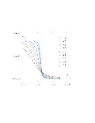
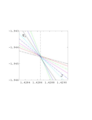
Figure 1: (a) The Binder cumulant $g_{r}$ from Eq. (8) as a function of the coupling $J$. The points are connected by splines to guide the eye. With increasing lattice size $L=12,16,20,24,30,36,48,60$ and $72$, the slope of the respective curve in the critical region increases. The vertical dashed line denotes our final result for $J_{c}$. (b) is an enlargement of (a) near the critical point. The dotted lines accompanying the solid/dashed lines show the jackknife error corridors.

first. We determine $T_{c}$ by studying the Binder cumulant $g_{r}$, which is a finite-size-scaling function

$$g_{r}\;=\;Q_{g}(tL^{1/\nu},L^{-\omega})~{}.$$ (10)

The function $Q_{g}$ depends on the thermal scaling field and on possible irrelevant scaling fields. In this case only the leading irrelevant scaling field proportional to $L^{-\omega}$ is specified, with an unknown $\omega>0$. Therefore, at the critical point ($t=0$) $g_{r}$ ought to be independent of $L$ apart from corrections due to these irrelevant scaling fields. Fig. 1 (a) shows our results for $g_{r}$. On the scale of Fig. 1 (a) we observe no deviation from the scaling hypothesis. After a blow-up of the close vicinity of the critical point, as shown in Fig. 1 (b), one sees that the intersection points $J_{ip}$ between the curves of different lattices are not coinciding perfectly at one $J$. These minor corrections to scaling have to be considered. By expanding the scaling function $Q_{g}$ to lowest order in both variables one gets for the intersection point $J_{ip}$ of two lattices with sizes $L$ and $L^{\prime}=bL$

$$J_{ip}(L,b)\;=\;J_{c}\,+\,c_{1}\,s(L,b)$$ (11)

with

$$s(L,b)\;=\;{1-b^{-\omega}\over b^{1/\nu}-1}L^{-\omega-1/\nu}~{}.$$ (12)

To have an unbiased estimate of $J_{c}$ we choose Binder’s approximation Binder

$${1\over J_{ip}}\;=\;{1\over J_{c}}\,+\,{c_{2}\over\ln b}~{},$$ (13)

which can be used without knowing the values of $\nu$ and $\omega$. In Fig.

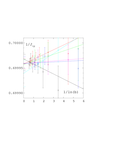
Figure 2: The coupling $J_{ip}$ at the intersection point of $g_{r}(L)$ and $g_{r}(bL)$ for various $L$ and $b$ as a function of $1/\ln b$, Eq. (13). The lines are linear fits for the lattices $L=12$ (black), $16$ (red), $20$ (green), $24$ (pink), $30$ (dark blue) and $36$ (light blue) through the intersection points with all larger lattices. The errors of the endpoints are drawn on the ordinate.

2 the $1/J_{ip}$ values of the intersection points from the lattices $L=12,16,20,24,30,36$ with all other larger lattices are plotted as a function of the variable $1/\ln b$ of Eq. (13). Linear fits should lead to the same value $1/J_{c}$ within the errors. Fitting the results to a constant value and varying the used $L$-values we find

$${1\over J_{c}}\;=\;0.699960(14),$$ (14)

which is equivalent to

$$J_{c}\;=\;1.42865(3).$$ (15)

This result agrees in the first four digits with the result $J_{c}=1.42895(6)$ of Butera and Comi Butera:1998rk . There is a slight difference in the last two digits. As this difference is larger than the corresponding errors, we check our result with the $\chi^{2}$-method Engels:1995em described in the following.
Let us review the general form of the scaling relations for different observables $\cal O$

$${\cal O}\;=\;L^{\rho/\nu}\,Q_{\cal O}\,(tL^{1/\nu},L^{-\omega}),$$ (16)

where we only take the largest irrelevant exponent into account. Here $\cal O$ is $M$, $\chi$ or $g_{r}$ with $\rho=-\beta,\gamma$ and $0$ respectively. Expanding the function $Q_{\cal O}$ to first order in the variables we find

$${\cal O}\!\!\!\!\!\!\! = \!\!\!\!\!\!\!L^{\rho/\nu}\,(c_{0}\,+\,(c_{1}\,+c_{2}L^{-\omega})\,tL^{1/\nu}$$ (17)

$${}\!\!\!\!\!\!\!+\,c_{3}L^{-\omega}),$$

which reduces to

$${\cal O}\;=\;L^{\rho/\nu}\,(c_{0}\,+\,c_{3}L^{-\omega})$$ (18)

at the critical point $t=0$. Therefore at the critical coupling a fit with equation (18) has the minimal $\chi^{2}$. Since we do not know the influence of $c_{3}L^{-\omega}$ we started without this correction term leaving $L=12$ out. Fig. 3 (a) shows the result. we find a deviation from our preliminary result in case of the magnetisation $M$ and the susceptibility $\chi_{v}$. The minima from the Binder cumulant and the susceptibility $\chi$ however coincide at $J\approx 1.42865$.

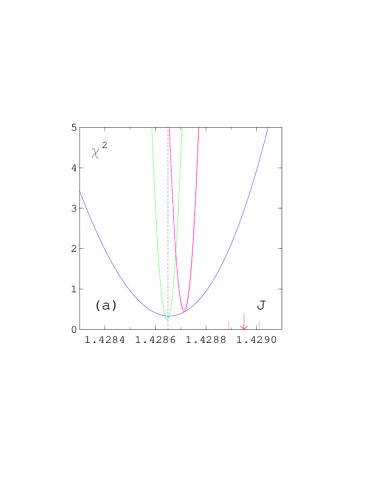
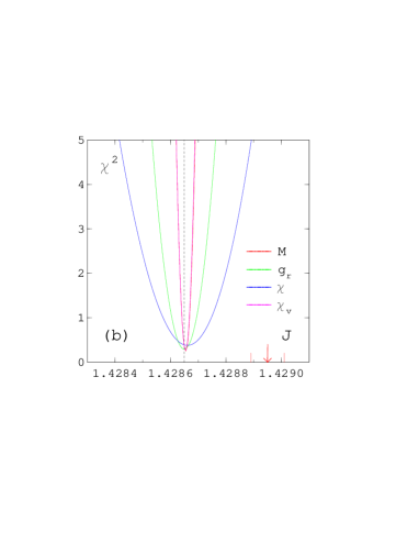
Figure 3: The minimal $\chi^{2}$ per degree of freedom for fits according to equation (18) for $M$ (red), $\chi_{v}$ (pink), $\chi$ (blue) and $g_{r}$ (green). Figure (a) shows the results without a correcting term $\propto L^{-\omega}$, whereas figure (b) uses $\omega=0.5$. The dotted black lines show our previous value of $J_{c}$, the arrows the result of Butera:1998rk with its error bars. The curves of $M$ and $\chi_{v}$ lie on top of each other.

We thereafter made fits with the correction term in the range $\omega=0.5-1.5$. The minimal $\chi^{2}$ and a perfect agreement of $J_{c}$ for all observables is found at $\omega=0.5$. This result is plotted in Fig. 3 (b). $\chi^{2}/d.o.f.$ increases with $\omega$ and shifts $J_{c}$ in case of $M$ and $\chi_{v}$ to smaller couplings, while the position calculated from $\chi$ increases and $J_{c}$ from $g_{r}$ remains nearly constant. Since the fits get worse we can exclude $\omega$-values larger than $0.8$. The positions of $J_{c}$ for $0.5\leq\omega\leq 0.8$ coincide within the error bars of Eq. (15).
At the critical point the Binder cumulant has the form

$$g_{r}(L)\;=\;g_{r}(J_{c})\,+\,c_{3}L^{-\omega},$$ (19)

with the universal value $g_{r}(J_{c})$ and a small correction term $c_{3}L^{-\omega}$. For fits with different $\omega$ we find $g_{r}$

$$g_{r}(J_{c})\;=\;-1.94456(10).$$ (20)

The quality of the fits does not change much ($\chi^{2}/d.o.f.\approx 0.2-0.3$) with different $\omega$ so a better estimate of $\omega$ is still not possible.

II.2 The critical exponents

Figure 4: The magnetisation $M$ as a function of the lattice extension $L$ at the critical point $T_{c}$ and $H=0$. The dashed line in is a fit to the ansatz (21) with $\omega=0.5$.

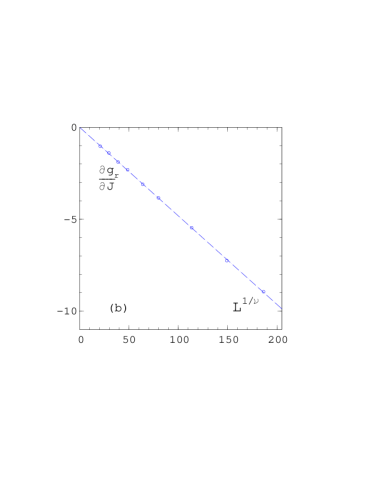
Figure 5: The derivative of the binder cumulant $\partial g_{r}/\partial J$ as a function of the lattice extension $L$ at the critical point $T_{c}$ and $H=0$. The dashed line is a fit to the ansatz (24) with $d_{3}=0$ since the corrections are negligible.

Since we now know the critical coupling we can study the finite-size behaviour of several observables with Eq. (18). These can be extracted from our reweighted data at $T_{c}$. The studied scaling relations are

$$M\!\! \!=\! \!\!L^{-{\beta/\nu}}\,(a_{0}\,+\,a_{3}L^{-\omega}),$$ (21)

$$\chi\!\! \!=\! \!\!L^{\gamma/\nu}\,(b_{0}\,+\,b_{3}L^{-\omega})$$ (22)

with $\omega\in[0.5;1.0[$ and the exponents $-\beta/\nu$ and $\gamma/\nu$ as free parameters. Since these two ratios are connected by the hyperscaling relation

$${\gamma\over\nu}\;=\;3\,-\,{2\beta\over\nu},$$ (23)

it is necessary to study a further observable, for example the derivative of $g_{r}$, which is given at $T_{c}$ by

$${\partial g_{r}\over\partial J}\;=\;L^{1/\nu}\,(d_{0}\,+\,d_{3}L^{-\omega}).$$ (24)

In this way two independent exponents (e.g. $\beta$ and $\nu$) can be estimated. We fit all observables in the range $L=12-72$. From Eq. (21) we obtain

$${\beta\over\nu}\;=\;0.519(2),$$ (25)

in which the error also includes an $\omega$-variation in $[0.5,1.0[$. Here a

Source			exponent	this work	Butera:1998rk	Antonenko:1998es	Gracey:1991zq ; Graceypc
$\partial g_{r}/\partial J$	$1/\nu$	1.223(5)	$\nu$	0.818(5)	0.819(3)	0.790	0.819
$M$	$\beta/\nu$	0.519(2)	$\beta$	0.425(2)	0.424(5)	0.407	0.424
$\chi$	$\gamma/\nu$	1.961(3)	$\gamma$	1.604(6)	1.608(4)	1.556	1.609

Table 2: The critical exponents for the $O(6)$ model estimated in this work compared to the theoretical work of Butera and Comi Butera:1998rk , Antonenko and Sokolov Antonenko:1998es and Gracey Gracey:1991zq ; Graceypc .

larger $\omega$ shifts $\beta/\nu$ to a smaller value at nearly constant $\chi^{2}/d.o.f.\approx 0.4$. Fig. 4 shows the result with $\omega=0.5$.
Our $\chi$-fits yield

$${\gamma\over\nu}\;=\;1.961(3).$$ (26)

Our results of $\beta/\nu$ and $\gamma/\nu$ are tested with the hyperscaling relation

$$2{\beta\over\nu}\,+\,{\gamma\over\nu}\;=\;d,$$ (27)

with $d=3$ being the dimension of the model. The left hand side of this equation is $2.999(5)$, correct within the error.
Finally we analyse the derivative $\partial g_{r}/\partial J$ of the Binder cumulant at $T_{c}$. This observable is directly calculated from the spline connection of our reweighted data in the neighbourhood of the critical point. The errors are obtained with the jackknife method, which seems to underestimate the errors, so we therefore assume the largest error of the different $L$-values for each lattice. Our fit to ansatz (24) without corrections to scaling ($\chi^{2}/d.o.f.\approx 0.3$) is shown in Fig. 5. For $d_{3}=0$ we find

$${1\over\nu}\;=\;1.223(5).$$ (28)

The final results of the critical exponents are summarized in Table 2. $\beta$ and $\gamma$ are calculated with the result of $\nu$ and the ratios (25) and (26). The three last columns of the table show the results from Butera:1998rk , Antonenko:1998es and Gracey:1991zq ; Graceypc . Butera and Comi as well as Gracey are in good agreement with our values, but the results of Antonenko and Sokolov are farther away.
In the following Sections we use the fixed critical exponents $\beta=0.425$ and $\nu=0.818$. The remaining critical exponents are calculated by the respective hyperscaling relations between the critical exponents. For $\omega$ we will use the value $\omega=0.5$, which seems to be the best estimate in all investigations.

III Simulations at $H>0$

The magnetisation $M$ is now calculated from equation (3). A transversal and a longitudinal susceptibility can be defined as

$$\chi_{L}\; = \;V(\langle\>M^{2}\>\rangle\,-\,M^{2})~{},$$ (29)

$$\chi_{T}\; = \;V\langle\>(\vec{\phi}^{\perp})^{2}\>\rangle~{}.$$ (30)

We simulated at several constant $J$-values and increasing magnetic field, starting at $H=0.00025$. The used lattice sizes were $L=24,36,48,72,96$ and $120$. Around $20,000$ measurements were performed in the $(J,H)$-regions we used for our fits. The only exception was the data of $L=120$, where we performed $10,000$ measurements at $J_{c}$ and $5,000$ measurements at all other $J$-values. The integrated autocorrelation time for the energy and the magnetisation is strongly dependent on the used $J$-values. At $J_{c}$ and $J>J_{c}$ we increased the number of cluster updates between two measurements to have autocorrelation times $\tau_{int}\raise 1.29167pt\hbox{$<$\kern-7.5pt\raise-4.73611pt\hbox{$\sim$}}6$.
In the symmetric phase ($J<J_{c}$) the situation is different. While the measurements of the magnetisation are less correlated with $\tau_{int}(M)\raise 1.29167pt\hbox{$<$\kern-7.5pt\raise-4.73611pt\hbox{$\sim$}}4$, the correlation of the energy increases rapidly with decreasing $H$ and $J$. It reaches values of $\tau_{int}(E)\raise 1.29167pt\hbox{$<$\kern-7.5pt\raise-4.73611pt\hbox{$\sim$}}30$ for the larger lattices.

III.1 The critical isotherm

At the critical point the critical scaling of the magnetisation is given by

$$M(T_{c},H)\;=\;d_{c}H^{1/\delta}\,(1\,+\,d_{c}^{1}H^{\omega\nu_{c}})~{},$$ (31)

where non-analytic corrections from the leading irrelevant scaling field are taken into account. They are not negligible in our model. The critical exponents $\delta$ and $\nu_{c}$ are known from the hyperscaling relations and only depend on the ratio $\beta/\nu=0.519(2)$:

$$\delta\; = \;3{\nu\over\beta}-1\;=\;4.780(22),$$ (32)

$$\nu_{c}\; = \;{\nu\over\beta\delta}\;=\;0.4031(24).$$ (33)

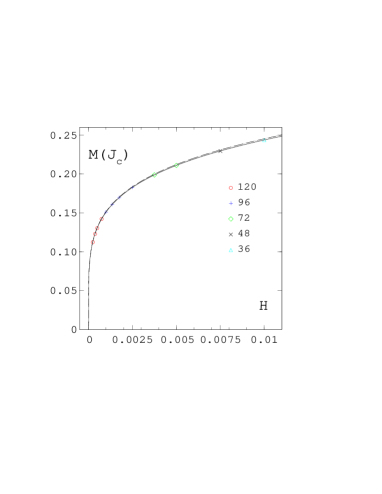
Figure 6: The magnetisation at the critical coupling as a function of $H$. The solid line is the fit to the ansatz (31), while the dashed line is the leading term.

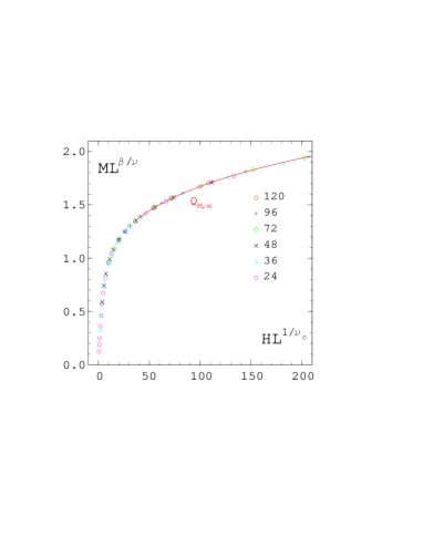
Figure 7: The finite-size-scaling function $Q_{M,\infty}$ on the critical line, Eq. (37). The solid red line indicates the asymptotic function $Q_{0,\infty}$ for $z^{\prime}\raise 1.29167pt\hbox{$>$\kern-7.5pt\raise-4.73611pt\hbox{$\sim$}}40$.

In order to exclude finite-size effects we carry out a reweighting analysis for all lattices and fit the result from the largest lattice to approximate the value of $V\to\infty$. This is done for the interval $H\in[0.00075;0.04]$ and we find

$$d_{c}=0.642(1).$$ (34)

Our result is plotted in Fig. 6. There are minimal negative corrections. If one treats $\delta$ as a free parameter the result $\delta=4.79(1)$ agrees with our first estimate.
The finite-size-scaling function for the magnetisation is

$$M(T,H,L)\!\!\!\!\!\!\!\! = \!\!\!\!\!\!\!\!L^{-\beta/\nu}\cdot$$ (35)

$$\!\!\!\!\!\!\!\!\Phi(tL^{1/\nu},HL^{1/\nu_{c}},L^{-\omega}).$$

The scaling function $\Phi$ can be expanded in $L^{-\omega}$ to

$$M(T,H,L)\!\!\!\!\!\!\!\! = \!\!\!\!\!\!\!\!L^{-\beta/\nu}\,\Phi_{0}(tL^{1/\nu},HL^{1/\nu_{c}})$$ (36)

$${}\!\!\!\!\!\!\!\!+\dots\;.$$

At $T_{c}$ the leading part is now given by

$$M(T_{c},H,L)\;=\;L^{-\beta/\nu}\,Q_{M}(z^{\prime})$$ (37)

with the universal scaling function $Q_{M}(z^{\prime})$ and the argument $z^{\prime}=HL^{1/\nu_{c}}$. The results of all lattices are shown in Fig. 7. The data points scale very well and the influence of corrections to scaling is small. In the limit $z^{\prime}\to\infty$ we expect the asymptotic behaviour

$$Q_{M,\infty}(z^{\prime})\;=\;d_{c}\,z^{\prime 1/\delta},$$ (38)

which is observable for $z^{\prime}\raise 1.29167pt\hbox{$>$\kern-7.5pt\raise-4.73611pt\hbox{$\sim$}}40$. This way one checks the value of $d_{c}$ with a fit of reweighted $z^{\prime}$-data of the larger lattices $L=72,96,120$. We find $d_{c}=0.642(1)$, which agrees perfectly with our first value of $d_{c}$.

III.2 Numerical results at $T\neq T_{c}$

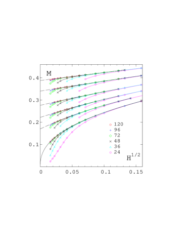
Figure 8: The magnetisation in the broken phase as a function of $\sqrt{H}$ for the couplings $J=1.6$, $1.55,1.50,1.47,1.45$ and $J_{c}$ and different lattices, starting with the largest $J$-value at the top. The solid lines represent interpolations from a reweighting analysis of the data. The dashed lines are the fits to ansatz (41) while the dotted line is the fit of equation (31) at $J_{c}$.

Let us review some perturbative predictions for the magnetisation and the susceptibilities. The continuous $O(6)$ symmetry of our spin model gives rise to spin waves, which are slowly varying (long-wavelength) spin configurations with energies arbitrarily close to the ground-state energy. In $d>2$ they are massless Goldstone modes associated with the spontaneous breaking of the rotational symmetry for temperatures below the critical value $T_{c}$ spin . For $T<T_{c}$ the system is in a broken phase, i.e. the magnetisation $M(T,H)$ attains a finite value $M(T,0)$ at $H=0$.
The transverse susceptibility has the form

$$\chi_{T}\;=\;\frac{M(T,H)}{H}$$ (39)

for all $H$ and $T$. This relation is a direct consequence of the $O(6)$ invariance of the zero-field free energy and can be derived as a Ward identity Brezin .

$J=1/T$	$M(T,0)$	$c_{1}(T)$	$c_{2}(T)$	$10^{4}\cdot H$	$\chi^{2}/dof$
1.45	0.1701(03)	1.339(15)	-2.86(18)	9-25	0.45
1.47	0.2219(02)	0.924(02)	-1.138(14)	12-74	0.56
1.50	0.2761(01)	0.659(01)	-0.436(08)	10-93	0.27
1.55	0.3401(01)	0.463(01)	-0.141(02)	10-163	0.78
1.60	0.3878(01)	0.363(01)	-0.047(01)	19-175	0.49

Table 3: Parameters of the fit of $M(T<T_{c},0)$ to the ansatz (41). The fifth column is the used fit range.

The longitudinal susceptibility diverges on the coexistence curve for $2<d\leq 4$ goldstone ; WZ . The leading terms in the perturbative expansion for three dimensions are

$$\chi_{L}(T<T_{c},H)\;=\;b_{0}(T)\,H^{-1/2}\,+\,c_{2}(T)~{}.$$ (40)

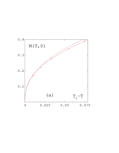
Figure 9: Magnetisation M(T,0) on the coexistence curve as a function of $(T_{c}-T)$. The red line is the fit to ansatz (42) while the black dashed line is the leading part.

Since the susceptibility is the derivative of the magnetisation with respect to $H$ we find for the magnetisation

$$M(T<T_{c},H)\!\!\!\!\!\!\!\! = \!\!\!\!\!\!\!\!M(T,0)\,+\,c_{1}(T)\,H^{1/2}$$ (41)

$$\!\!\!\!\!\!\!\!+\,c_{2}(T)\,H$$

near the coexistence curve. Fig. 8 shows our results of the magnetisation in the broken phase and the corresponding extrapolations to $M(T,0)$ in the thermodynamic limit ($V\to\infty$). The numbers of the parameters are presented in Table 3. The $H$-extension of the regions, where the predicted Goldstone behaviour is found, increases with $J$, while finite-size effects become larger at small $H$ and larger $J$ ($L\raise 1.29167pt\hbox{$>$\kern-7.5pt\raise-4.73611pt\hbox{$\sim$}}160$ would be necessary for finite-size independent data).
We fitted the values of $M(T,0)$ to the form

$$M(T\mathrel{\hbox to0.0pt{\lower 3.0pt\hbox{$\mathchar 536\relax$}\hss}\raise 2.0pt\hbox{$\mathchar 316\relax$}}T_{c},0)\!\!\!\!\!\!\!\! = \!\!\!\!\!\!\!\!B\,(T_{c}-T)^{\beta}[1\,+\,b_{1}\,(T_{c}-T)^{\omega\nu}$$ (42)

$$\!\!\!\!\!\!\!\!{}+\,b_{2}\,(T_{c}-T)]$$

with fixed values $\beta=0.425$, $\omega\nu=0.409$ and the result

$$B=1.22(1),$$ (43)

$b_{1}=-0.184(49)$ and $b_{2}=0.31(13)$. The error of $B$ also

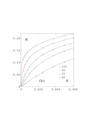
Figure 10: The magnetisation in the symmetric phase ($T\geq T_{c}$) as a function of $H$, starting from the top with fixed $J=J_{c},1.42,1.41,1.40$ and $1.38$ and different $L$-values. The lines are spline connections between the data points.

includes the slight uncertainty in the value of $\omega\nu$. Our final result of $M(T,0)$ and the difference to the leading term are plotted in Fig. 9.
Since one of the main aims of this work is the determination of the magnetic equation of state in Section IV, we also simulated in the high temperature phase. Again we use data of the largest lattices as an approximation for the infinite volume value. The result is plotted in Fig. 10. From a Taylor expansion we expect

$$M(T>T_{c},H)\;\propto\;H.$$ (44)

at small $H$. With increasing temperature the $H$-interval with this behaviour increases, as one can see in Fig. 10.

IV The Scaling function

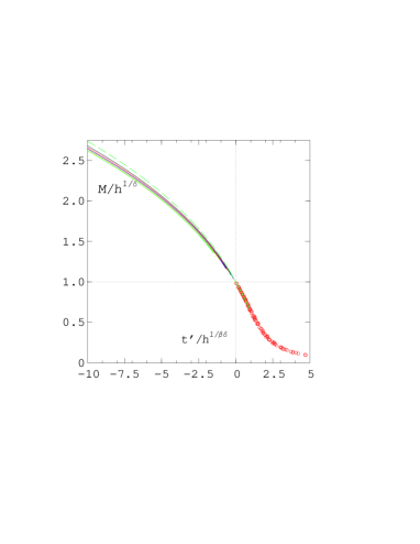
Figure 11: The function $M/h^{1/\delta}$. The solid lines in the broken phase are the reweighted results for $M/h^{1/\delta}$ at $J=1.60,1.55,1.50,1.47,1.45,1.445$ and $1.44$, from the bottom to the top. They are extrapolated with Equation (55) to $f_{G}$ (dashed line). The circles are single data points in the symmetric phase.

The critical behaviour of the magnetisation in the vicinity of $T_{c}$ is described by the general Widom-Griffiths form Griffiths

$$y\;=\;f(x)$$ (45)

with

$$y\equiv h/M^{\delta},\quad x\equiv t^{\prime}/M^{1/\beta},$$ (46)

where the variable $t^{\prime}$ is proportional to $(T-T_{c})$ and $h$ proportional to $H$. A common normalisation of the function $f(x)$ is

$$f(0)=1,\quad f(-1)=0.$$ (47)

The variables $t^{\prime}$ and $h$ are the conveniently normalized reduced temperature $t^{\prime}=(T-T_{c})/T_{0}$ with $T_{0}=B^{-1/\beta}=0.626(12)$ and the reduced magnetic field $h=H/H_{0}$ using $H_{0}=d_{c}^{-\delta}=8.32(6)$. The function $f(x)$ is universal and was derived from the $\epsilon$-expansion ($\epsilon=4-d$) to order $\epsilon^{2}$ Brezin . In the limit $x\to-1$, i.e. at $T<T_{c}$ and close to $H=0$ the result was inverted to give $x+1$ as a double expansion in powers of $y$ and $y^{d/2-1}$ WZ

$$x+1\!\!\!\!\!\!\!\! = \!\!\!\!\!\!\!\!{\widetilde{c}_{1}}y\,+\,{\widetilde{c}_{2}}y^{d/2-1}\,+\,{\widetilde{d}_{1}}y^{2}$$ (48)

$${}\!\!\!\!\!\!\!\!+\,{\widetilde{d}_{2}}y^{d/2}\,+\,{\widetilde{d}_{3}}y^{d-2}\,+\,\ldots\;.$$

The coefficients ${\widetilde{c}_{1}}$, ${\widetilde{c}_{2}}$ and ${\widetilde{d}_{3}}$ are thereafter obtained from the general expression of Brezin .
In the large-$x$ limit (corresponding to $T>T_{c}$ and small $H$), the expected behaviour is given by Griffiths’s analyticity condition Griffiths

$$f(x)\;=\;\sum_{n=1}^{\infty}a_{n}\,x^{\gamma-2(n-1)\beta}\,.$$ (49)

The form (45) of the equation of state is equivalent to the often used relation

$$M\;=\;h^{1/\delta}f_{G}(z),$$ (50)

where $f_{G}$ is a further universal scaling function and $z$ the combination

$$z\;=\;t^{\prime}/h^{1/\beta\delta}.$$ (51)

The normalisation conditions of $f_{G}(z)$ are

$$f_{G}(0)\;=\;1~{}\quad{\rm and}\quad f_{G}(z)\stackrel{{\scriptstyle z\rightarrow-\infty}}{{\longrightarrow}}(-z)^{\beta}~{}.$$ (52)

This version is normally used for comparison to QCD lattice data. The function $f(x)$ is connected with $f_{G}(z)$ by

$$y=f_{G}^{-\delta},\quad x=z\,f_{G}^{-1/\beta}.$$ (53)

These scaling functions are only valid close to $J_{c}$ and $H\to 0$. First tests show that the data we have used in the broken phase does not scale directly, while in the high temperature phase most of the data scales close to $T_{c}$ and small $H$. So we used a more general form of (50)

$$Mh^{-1/\delta}\;=\;\Psi(z,h^{\omega\nu_{c}})$$ (54)

with a scaling function $\Psi$, which can be expanded to

$$Mh^{-1/\delta}\;\!\!\!\!\!\!\!\! = \!\!\!\!\!\!\!\!\;f_{G}(z)\,+\,h^{\omega\nu_{c}}f_{G}^{(1)}(z)$$ (55)

$$\!\!\!\!\!\!\!\!{}+\,h^{2\omega\nu_{c}}f_{G}^{(2)}(z)\,+\,\dots\,.$$

This way in the broken phase one obtains the leading part $f_{G}$ by quadratic fits to our data in $h^{\omega\nu_{c}}$ at constant $z$-values and different $(J/H)$-combinations. But we are only able to correct the data with $z\mathrel{\hbox to0.0pt{\lower 3.0pt\hbox{$\mathchar 536\relax$}\hss}\raise 2.0pt\hbox{$\mathchar 316\relax$}}-2$ because we have not enough $J$-values closer to $J_{c}$ to make the fits. In Fig. 11 we show the influence of the corrections and the final scaling function $f_{G}$ in the broken phase (dashed

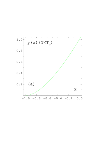
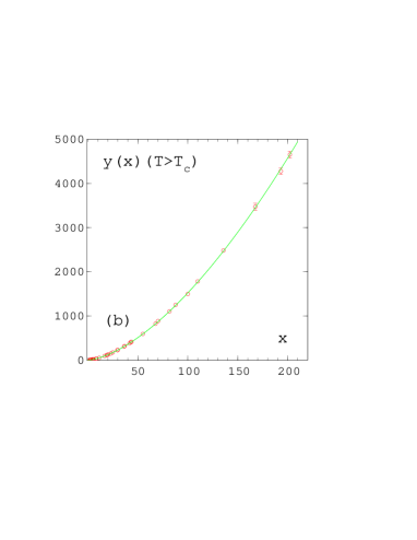
Figure 12: The functions $y=f(x)$ at small $x$ (a) and large $x$-values (b). In figure (a) we plot the fit to ansatz (56) using extrapolated data in the broken phase and data-points in the symmetric phase. In (b) we plot data-points of the symmetric phase and the fit to ansatz (49) using the first three terms.

line).
Our result for $f_{G}(z)$ can be transformed with (53) into the Widom-Griffiths form of the equation of the state (45). Unfortunately the $z$-interval we used to extract $f_{G}(z)$ is only equivalent to the small region $-0.9\mathrel{\hbox to0.0pt{\lower 3.0pt\hbox{$\mathchar 536\relax$}\hss}\raise 2.0pt\hbox{$\mathchar 316\relax$}}x\mathrel{\hbox to0.0pt{\lower 3.0pt\hbox{$\mathchar 536\relax$}\hss}\raise 2.0pt\hbox{$\mathchar 316\relax$}}-0.7$, which can be used for a fit. We use the three leading terms in (48)

$$x_{1}(y)+1\!\!\!\!\!\!\!\! = \!\!\!\!\!\!\!\!({\widetilde{c}_{1}}\,+\,{\widetilde{d}_{3}})\,y\,+\,{\widetilde{c}_{2}}\,y^{1/2}$$ (56)

$${}\!\!\!\!\!\!\!\!+\,{\widetilde{d}_{2}}\,y^{3/2}\;.$$

Since $y(0)=1$ the coefficients are connected by ${\widetilde{d}_{2}}=1-({\widetilde{c}_{1}}\,+\,{\widetilde{d}_{3}}\,+\,{\widetilde{c}_{2}})$. Fits to $x$ in the interval $-0.9\mathrel{\hbox to0.0pt{\lower 3.0pt\hbox{$\mathchar 536\relax$}\hss}\raise 2.0pt\hbox{$\mathchar 316\relax$}}x\mathrel{\hbox to0.0pt{\lower 3.0pt\hbox{$\mathchar 536\relax$}\hss}\raise 2.0pt\hbox{$\mathchar 316\relax$}}-0.7$ and points in the symmetric phase with $0.2\mathrel{\hbox to0.0pt{\lower 3.0pt\hbox{$\mathchar 536\relax$}\hss}\raise 2.0pt\hbox{$\mathchar 316\relax$}}x\mathrel{\hbox to0.0pt{\lower 3.0pt\hbox{$\mathchar 536\relax$}\hss}\raise 2.0pt\hbox{$\mathchar 316\relax$}}2.9$, $1.4\mathrel{\hbox to0.0pt{\lower 3.0pt\hbox{$\mathchar 536\relax$}\hss}\raise 2.0pt\hbox{$\mathchar 316\relax$}}J<J_{c}$ and $H\leq 0.0015$ lead to

$${\widetilde{c}_{1}}+{\widetilde{d}_{3}}\,=\,0.36(5)\;,\quad{\widetilde{c}_{2}}\,=\,0.69(3).$$ (57)

The result of the fit is shown by the line in Fig. 12(a).
For large $x$ we use a 3-parameter fit of the first three terms of Griffiths’s analyticity condition (49)

$$y_{2}(x)\;=\;a_{1}x^{\gamma}\,+\,a_{2}x^{\gamma-2\beta}\,+\,a_{3}x^{\gamma-4\beta}$$ (58)

in the interval $x\in[1.75,202]$ and data points restricted to $1.4\mathrel{\hbox to0.0pt{\lower 3.0pt\hbox{$\mathchar 536\relax$}\hss}\raise 2.0pt\hbox{$\mathchar 316\relax$}}J<J_{c}$ and $H\leq 0.0015$. We find

$$a_{1}\,=\,0.92(1)\,,\quad a_{2}\,=\,1.17(2)\,,$$

$$\quad\quad\quad\quad a_{3}\,=\,0.91(3).$$ (59)

This result is plotted in Fig. 12(b). With the coefficient $a_{1}$ of the leading part one can calculate the universal ratio

$$R_{\chi}\;=\;a_{1}^{-1}\;=\;1.09(1).$$ (60)

The $O(6)$ scaling function $f_{G}$ can be parametrically obtained from $x_{1}(y)$

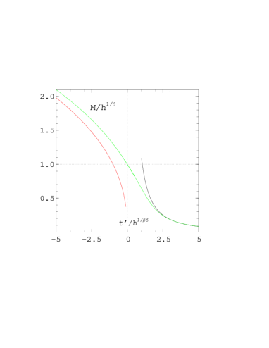
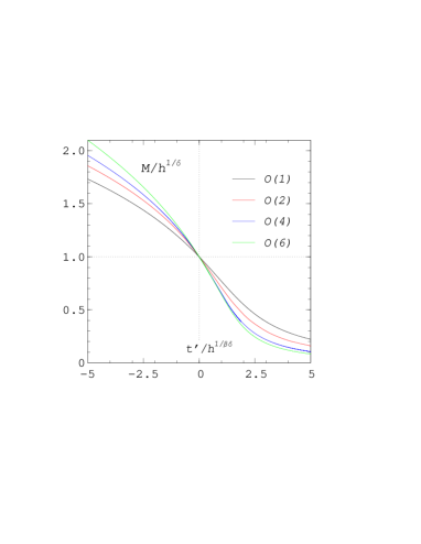
Figure 13: (a) The scaling function $f_{G}$ of the O(6) model (green) and the asymptotic behaviours for $z\to\infty$ (black) and $z\to-\infty$ (red). (b) The scaling function $f_{G}$ for the Ising (black), $O(2)$ (red), $O(4)$ (blue) and $O(6)$ model (green).

and $y_{2}(x)$, which is connected by a spline between $z=0.5$ and $z=0.8$, where we have no reliable parametrisation. The result is plotted in Fig. 13(a). Also plotted are the leading terms of the asymptotic behaviour at $z\to\pm\infty$. These are

$$f_{G}(z)\!\! \stackrel{{\scriptstyle z\rightarrow-\infty}}{{=}} \!\!(-z)^{\beta}~{},$$ (61)

$$f_{G}(z)\!\! \stackrel{{\scriptstyle z\rightarrow+\infty}}{{=}} \!\!R_{\chi}z^{-\gamma}$$ (62)

according to the normalisation (52). The fact that for large temperatures and small $H$ the magnetisation is proportional to $H$, see Eq. (44), explains the asymptotic behaviour for $z\to\infty$. In the symmetric phase the asymptotic behaviour is reached for small absolute values of $z$, while in the broken phase the scaling function converges to the asymptotic form not until large absolute values of $z$.
Finally, the $O(6)$ scaling function $f_{G}$ can be compared to the corresponding functions for the Ising ($O(1)$) model Engels:2002fi , the $O(2)$ Engels:2000xw and the $O(4)$ model Engels:1999wf , shown in Fig. 13(b). All functions have a similar shape.

V The Pseudocritical Line

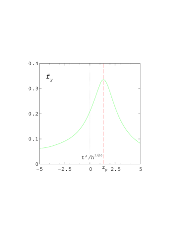
Figure 14: The scaling function $f_{\chi}$ for the $O(6)$ model. The dashed red line shows the position of $z_{p}=1.34$.

In order to discuss finite-size-scaling functions in an easier way, it is common to study lines of constant $z$-values. There one expresses $H$ as a function of $T$ or vice versa. Important examples of lines of fixed $z$ are the critical line ($z=0$), discussed in Section III.1, and the pseudocritical line $z=z_{p}=const$, the line of peak positions of the susceptibility $\chi_{L}$ in the $(t,h)$-plane for $V\rightarrow\infty$. There are two different ways to find that value of $z_{p}$ for $O(N)$ models. One way is to locate the peak positions of $\chi_{L}$ as a function of the temperature at different fixed small values of the magnetic field on lattices with increasing size $L^{3}$. The scaling function, on the other hand, offers a more elegant way to determine the pseudocritical

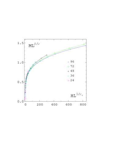
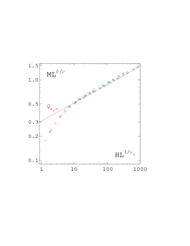
Figure 15: (a) Finite-size scaling of $ML^{\beta/\nu}$ on the pseudocritical line. (b) is a double-log plot of (a). The solid line in (b) shows the asymptotic form $Q_{z_{p},\infty}$, the symbols denote different lattice sizes $L$.

line. Since $\chi_{L}$ is the derivative of $M$

$$\chi_{L}={\partial M\over\partial H}={h^{1/\delta-1}\over H_{0}}f_{\chi}(z)~{},$$ (63)

its scaling function $f_{\chi}(z)$ can be calculated directly from $f_{G}(z)$

$$f_{\chi}(z)={1\over\delta}\left(f_{G}(z)-{z\over\beta}\frac{\partial f_{G}}{\partial z}(z)\right)~{}.$$ (64)

The maximum of $f_{\chi}(z)$ is located at $z_{p}$, which is another universal quantity. We find for the $O(6)$ model

$$z_{p}\;=\;1.34(5)\,.$$ (65)

The error includes the fit-errors of the parameters in (59).
In Fig. 14 we show the result for $f_{\chi}(z)$ from Eq. (64) in the $O(6)$ model.
At $z_{p}$ a finite-size-scaling analysis in the variables $H$ and $L$ can be performed. Eq. (36) reduces to

$$M(H,L)\;=\;L^{-\beta/\nu}\,Q_{z_{p}}(hL^{1/\nu_{c}})\,+\,\dots$$ (66)

with another universal scaling function $Q_{z_{p}}$. The asymptotic form $Q_{z_{p},\infty}$ of $Q_{z_{p}}$ is

$$Q_{z_{p}}\stackrel{{\scriptstyle L\rightarrow\infty~{}}}{{\longrightarrow}}Q_{z_{p},\infty}=f_{G}(z_{p})\,(hL^{1/\nu_{c}})^{1/\delta}\quad$$ (67)

The results are presented in Fig. 15(a). The data does not scale directly but with increasing volume the data-points approach $Q_{z_{p}}$ from the top. In Fig. 15(b) we plotted the data in a double-log form and find that the asymptotic form $Q_{z_{p},\infty}$ coincides with the $Q_{z_{p}}$-value of the largest lattice extension at $HL^{1/\nu_{c}}\mathrel{\hbox to0.0pt{\lower 3.0pt\hbox{$\mathchar 536\relax$}\hss}\raise 2.0pt\hbox{$\mathchar 318\relax$}}42$. Therefore $Q_{z_{p}}$ is asymptotic. At smaller values, one observes an approach of $Q_{z_{p}}$ from below to $Q_{z_{p},\infty}$.

VI Conclusions

In this paper we calculated several important quantities of the O(6) spin model directly from Monte Carlo simulations on cubic lattices. At zero external field we determined the critical coupling $J_{c}$ by a finite-size-scaling analysis of the Binder cumulant and by the $\chi^{2}$-method. Our result agrees in the first four digits with the result of Butera and Comi. At the critical point we estimated the critical exponents from finite-size-scaling fits. We obtained $\beta$ from the magnetisation, $\gamma$ from the susceptibility and $\nu$ from the derivative of the Binder cumulant. Our results are in accord with the values found by Butera and Comi but slightly different compared to the values found by Antonenko and Sokolov. We find small corrections to scaling for all observables.
On the critical line $T=T_{c},H>0$ and in the limit $V\to\infty$, the critical amplitude $d_{c}$ of the magnetisation was computed. We found small negative corrections to scaling and checked the finite-size-scaling behaviour of $M$ at $T_{c}$ and its asymptotic form.
Below the critical temperature, we investigated the behaviour of $M$ at several couplings $J$ as a function of $H^{1/2}$ in the limit $V\to\infty$. Close to the coexistence line, i.e. small $H\to 0$, the predicted Goldstone behaviour was observed. We were able to extrapolate our data to the values $M(T<T_{c};H=0)$ of the infinite volume limit, fitted these $M$-values with the corresponding ansatz, and estimated the critical amplitude $B$ of the magnetisation. In this case the corrections to scaling were again negative and more pronounced as on the critical line. At high temperatures and $H>0$, we observe the expected proportional dependence on $H$ of the magnetisation.
We used our data of the largest lattices in the low and high-temperature phase to parametrise the scaling function $f_{G}$ of the O(6) model. We encountered large corrections to scaling in the broken phase, while most data in the symmetric phase scales directly. By generalizing $f_{G}$ to include corrections to scaling, our group extracted a part of $f_{G}$ in the broken phase and fitted the result combined with direct data points in the symmetric phase. On the other hand, we fitted data of the symmetric phase using Griffiths’s analyticity condition. Finally, we compared our $O(6)$-result for $f_{G}$ with the corresponding scaling functions of the $O(1)$, $O(2)$ and $O(4)$ model. These functions are clearly distinguishable and in a systematic order. We use our result of $f_{G}$ to calculate the scaling function $f_{\chi}$ of the susceptibility. From the position of the maximum in $f_{\chi}$ the location of the pseudocritical line was determined. There we made finite-size-scaling plots and found considerable corrections to scaling. The data of smaller lattices approaches the universal finite-size-scaling function from above. The asymptotic form of the universal part is reached at $HL^{1/{\nu_{c}}}\approx 42$.
A comparison between the $O(6)$ model and aQCD will be done in the near future.

- (1) R. D. Pisarski and F. Wilczek, Phys. Rev. D 29, 338 (1984).
- (2) K. Rajagopal and F. Wilczek, Nucl. Phys. B 399, 395 (1993).
- (3) F. Wilczek, Int. J. Mod. Phys. A 7, 3911 (1992). [Erratum-ibid. A 7 (1992) 6951].
- (4) S. Aoki et al. [JLQCD Collaboration], Nucl. Phys. Proc. Suppl. 60A, 188 (1998)
- (5) S. Aoki, Y. Iwasaki, K. Kanaya, S. Kaya, A. Ukawa and T. Yoshie, Nucl. Phys. Proc. Suppl. 63, 397 (1998).
- (6) J. Engels, S. Holtmann, T. Mendes and T. Schulze, Phys. Lett. B 514, 299 (2001).
- (7) F. Karsch and M. Lütgemeier, Nucl. Phys. B 550, 449 (1999).
- (8) A. L. Talapov and H. W. Blöte, J. Phys. A29, 5727 (1996).
- (9) J. Engels and T. Mendes, Nucl. Phys. B 572, 289 (2000).
- (10) J. Engels, S. Holtmann, T. Mendes and T. Schulze, Phys. Lett. B 492, 219 (2000).
- (11) A. Cucchieri, J. Engels, S. Holtmann, T. Mendes and T. Schulze, J. Phys. A 35, 6517 (2002).
- (12) P. Butera and M. Comi, Phys. Rev. B 58, 11552 (1998).
- (13) K. Binder, Phys. Rev. Lett. 47, 693(1981).
- (14) J. Engels, S. Mashkevich, T. Scheideler and G. Zinovev, Phys. Lett. B 365, 219 (1996).
- (15) S. A. Antonenko and A. I. Sokolov, Phys. Rev. E 51, 1894 (1995).
- (16) J. A. Gracey, J. Phys. A 24, L197 (1991) [Erratum-ibid. A 35, 9701 (2002)].
- (17) J. A. Gracey (private communication).
- (18) V .G. Vaks, A .I. Larkin and S .A. Pikin, Sov. Phys. JETP 26, 647 (1968).
- (19) E. Brézin, D.J. Wallace and K.G. Wilson, Phys. Rev. B7, 232 (1973).
- (20) J. Zinn-Justin, Quantum Field Theory and Critical Phenomena (Clarendon Press, Oxford, 1996); R. Anishetty et al., Int. J. Mod. Phys. A14, 3467 (1999).
- (21) D. J. Wallace and R. K. P. Zia, Phys. Rev. B 12, 5340 (1975).
- (22) R. B. Griffiths, Phys. Rev. 158, 176 (1967).
- (23) J. Engels, L. Fromme and M. Seniuch, Nucl. Phys. B 655, 277 (2003).