The Supersymmetric Ward-Takahashi Identity in 1-Loop
Lattice Perturbation Theory: General Procedure

Abstract

The one-loop corrections to the lattice supersymmetric Ward-Takahashi identity (WTi) are investigated in the off-shell regime. In the Wilson formulation of the $N=1$ supersymmetric Yang-Mills (SYM) theory, supersymmetry (SUSY) is broken by the lattice, by the Wilson term and is softly broken by the presence of the gluino mass. However, the renormalization of the supercurrent can be realized in a scheme that restores the continuum supersymmetric WTi (once the on-shell condition is imposed). The general procedure used to calculate the renormalization constants and mixing coefficients for the local supercurrent is presented. The supercurrent not only mixes with the gauge invariant operator $T_{\mu}$. An extra mixing with other operators coming from the WTi appears. This extra mixing survives in the continuum limit in the off-shell regime and cancels out when the on-shell condition is imposed and the renormalized gluino mass is set to zero. Comparison with numerical results are also presented.

I Introduction

SUSY or fermion-boson symmetry is one of the most exciting topics in field theory. From a theoretical point of view SUSY plays a fundamental role in string theory. There are many strong phenomenological motivations for believing that SUSY is realized in Nature in a spontaneoulsy broken form. The SUSY breaking mechanisms are requested in order to produce a low energy 4-dimensional effective action with a residual $N=1$ SUSY. For the other hand, non-perturbative studies of supersymmetric gauge theories turn out to have remarkably rich properties which are of great physical interest, as has been pointed out in seiberg . For this reason, much effort has been dedicated to formulating a lattice version of supersymmetric theories (for a recent review in SUSY on the lattice with a complete list of relevant references, see feo5 ). More recently, related interesting results in SUSY can be found in hiller ; rey ; catterall ; beccaria ; campostrini ; campostrini2 ; itoh ; kaplan ; kaplan2 ; giedt . Some of these formulations try to realize chiral gauge theories on the lattice with an exact chiral gauge symmetry luscher1 ; luscher2 ; luscher3 ; luscher4 . The lattice formalism is a powerful tool to extract non-perturbative dynamics of field theories and may be able to provide additional information and confirm or improve theoretical expectations.

To formulate SUSY on the lattice we follow the ideas of Curci and Veneziano curci . They propose to give up manifest SUSY on the lattice, and instead, to restore it in the continuum limit. In curci , the Wilson formulation for the $N=1$ SYM theory, which is the simplest SUSY gauge theory and corresponds to the SUSY gluodynamics, is adopted. For SU$(N_{c})$ it has $(N_{c}^{2}-1)$ gluons and the same number of massless Majorana fermions (gluinos), in the adjoint representation of the color group.

SUSY is broken explicitly by the Wilson term and the finite lattice spacing. In addition, a soft breaking due to the introduction of the gluino mass is present. In curci it is proposed that SUSY can be recovered in the continuum limit by tuning the bare gauge coupling, $g_{0}$, and the gluino mass, $m_{\tilde{g_{0}}}$, to the SUSY point, $m_{\tilde{g_{0}}}=0$, which also coincides with the chiral point. In montvay ; pap ; kirchner ; kirchner2 ; campos ; farchioni ; montvay3 , the DESY-Münster-Roma Collaboration have investigated these issues for the $SU(2)$ gauge group (some first results have been obtained for $SU(3)$ feo2 ), simulating the theory with a dynamical gluino using the multi-bosonic algorithm luscher5 with a two-step variant called the (TSMB) algorithm montvay2 (while quenched results are in vladikas ).

Another independent way to study the SUSY (chiral) limit in the Wilson formulation of Curci and Veneziano, is through the study of the SUSY WTi. On the lattice, it contain explicit SUSY breaking terms and the SUSY limit is defined to be the point in the parameter space where these breaking terms vanish and the SUSY WTi recovers its continuum form. These issues have been investigated numerically in farchioni in the on-shell regime.

In this paper, the general procedure used to determine the renormalization constants and mixing coefficients for the local definition of the supercurrent, in the off-shell regime, is explained. It is shown that, when the operator insertion involves elementary fields, the supercurrent not only mixes with the gauge invariant operator $T_{\mu}$, as have been claimed in curci . The supercurrent contains also non-Lorentz covariant terms which survive in the continuum, in the off-shell regime. These non-Lorentz breaking terms cancel out when the on-shell condition on the gluino is imposed and the continuum SUSY WTi is recovered. Preliminary studies have been presented in feo ; feo4 .

The paper is organized as follows. In Sec. II the Curci and Veneziano lattice formulation of the $N=1$ SYM theory is presented, together with the lattice action and the vertices used for the calculation. In Sec. III the SUSY WTi on the lattice are written and the renormalization procedure explained. The calculation of the renormalization constant for the supercurrent is presented in Sec. IV. Discussions and outlook are summarized in Sec. V. In Appendices A, B and C, some details of the calculation are showed.

II Lattice Formulation

In the Wilson formulation of the $N=1$ SYM theory curci , the gluonic part of the action is the standard plaquette one

$$S_{g}=\frac{\beta}{2}\sum_{x}\sum_{\mu\nu}\bigg{(}1-\frac{1}{N_{c}}\mbox{Re}\,\mbox{Tr}\,P_{\mu\nu}(x)\bigg{)}\,,$$ (1)

where the plaquette operator is defined as muenster

$$P_{\mu\nu}(x)=U^{\dagger}_{\nu}(x)U^{\dagger}_{\mu}(x+\hat{\nu})U_{\nu}(x+\hat{\mu})U_{\mu}(x)\,,$$ (2)

and the bare coupling is given by $\beta\equiv 2N_{c}/g_{0}^{2}$. For Wilson fermions the fermionic part of the action reads

$$S_{f}=\sum_{x}a^{4}\mbox{Tr}\bigg{[}$$

$$\frac{1}{2a}\Bigg{(}\bar{\lambda}(x)(\gamma_{\mu}-r)U_{\mu}^{\dagger}(x)\lambda(x+a\hat{\mu})U_{\mu}(x)-$$

$$\bar{\lambda}(x+a\hat{\mu})(\gamma_{\mu}+r)U_{\mu}(x)\lambda(x)U_{\mu}^{\dagger}(x)\Bigg{)}+$$

$$\bigg{(}m_{0}+\frac{4r}{a}\bigg{)}\bar{\lambda}(x)\lambda(x)\bigg{]}\,,$$ (3)

where $m_{0}$ is the gluino bare mass and $a$ is the lattice spacing. The fermionic field (gluino), $\lambda(x)=\lambda^{a}(x)T^{a}$, is a Majorana spinor in the adjoint representation of the gauge group. The symbol Tr implies the trace over the color indices. The normalization is given by $\mbox{Tr}(T^{a}T^{b})=\frac{1}{2}\delta_{ab}$. In this paper, only the case $N_{c}=2$ is considered, for which the adjoint gluino field is expressed in terms of Pauli matrices $\sigma_{k}$ as

$$\lambda=\sum_{k=1}^{3}\frac{1}{2}\sigma_{k}\lambda^{k}\,.$$ (4)

The gluino field $\lambda(x)$ satisfies the Majorana condition

$$\lambda(x)=C\bar{\lambda}^{T}(x)\,,$$ (5)

where $C=\gamma_{2}\gamma_{0}$, is the charge conjugation operator. Our matrix convention for the Euclidean $\gamma$ matrices is as follow,

$$\gamma_{0}=\left(\begin{array}[]{cc}0&1\\ 1&0\end{array}\right)$$ (6)

and

$$\gamma_{k}=\left(\begin{array}[]{cc}0&-i\sigma^{k}\\ i\sigma^{i}&0\end{array}\right)\,.$$ (7)

The matrix $\gamma_{5}$ is defined to be

$$\gamma_{5}\equiv\gamma_{1}\gamma_{2}\gamma_{3}\gamma_{0}=\left(\begin{array}[]{cc}1&0\\ 0&-1\end{array}\right)$$ (8)

and the matrix $\sigma_{\mu\nu}$ is

$$\sigma_{\mu\nu}=\frac{i}{2}[\gamma_{\mu},\gamma_{\nu}]\,.$$ (9)

The anti-commutator property is

$$\big{\{}\gamma_{\mu},\gamma_{\nu}\big{\}}=2\delta_{\mu\nu}\,.$$ (10)

Finally, the Wilson parameter is fixed to be $r=1$.

SUSY is not realized on the lattice because, as the Poincaré algebra, a sector of the superalgebra, is lost. SUSY is explicitly broken in the action (1,3) by the lattice itself, by the gluino mass term and by the Wilson term. Nevertheless, one can still define some transformations that reduce to the continuum supersymmetric ones, in the limit $a\to 0$. One choice is taniguchi ; galla :

$$\delta U_{\mu}(x) = -ag_{0}U_{\mu}(x)\bar{\xi}(x)\gamma_{\mu}\lambda(x)-$$

$$ag_{0}\bar{\xi}(x)\gamma_{\mu}\lambda(x+a\hat{\mu})U_{\mu}(x)\,,$$

$$\delta U_{\mu}^{\dagger}(x) = ag_{0}\bar{\xi}(x)\gamma_{\mu}\lambda(x)U_{\mu}^{\dagger}(x)+$$

$$ag_{0}U_{\mu}^{\dagger}(x)\bar{\xi}(x)\gamma_{\mu}\lambda(x+a\hat{\mu})\,,$$

$$\delta\lambda(x) = -\frac{i}{g_{0}}\sigma_{\rho\tau}{\cal G}_{\rho\tau}(x)\xi(x)\,,$$

$$\delta\bar{\lambda}(x) = \frac{i}{g_{0}}\bar{\xi}(x)\sigma_{\rho\tau}{\cal G}_{\rho\tau}(x)\,,$$ (11)

where $\xi(x)$ and $\bar{\xi}(x)$ are infinitesimal Majorana fermionic parameters, while ${\cal G}_{\rho\tau}(x)$ is the clover plaquette operator,

$${\cal G}_{\rho\tau}(x) = -\frac{1}{8a^{2}}\bigg{(}P_{\rho\tau}(x)-P_{\tau\rho}(x)+$$ (12)

$$P_{-\rho,-\tau}(x)-P_{-\tau,-\rho}(x)+P_{\tau,-\rho}(x)-$$

$$P_{-\rho,\tau}(x)+P_{-\tau,\rho}(x)-P_{\rho,-\tau}(x)\bigg{)}\,.$$

Weak coupling perturbation theory is developed by writing the link variable as

$$U_{\mu}(x)=e^{-aA_{\mu}(x)}\,,$$ (13)

and expanding it in terms of $g_{0}$. Here the gluon field is defined to be $A_{\mu}(x)=-ig_{0}A_{\mu}^{b}(x)T^{b}$.

In order to calculate the 1-loop corrections to the SUSY WTi (which correspond to $O(g_{0}^{2})$), we need two kinds of gluon-gluino interaction vertices. The gluon-gluino vertex,

$$V_{1\mu}^{ab,c}(p,q) = g_{0}f^{abc}\bigg{[}\gamma_{\mu}\cos(\frac{p_{\mu}a}{2}+\frac{q_{\mu}a}{2})-$$ (14)

$$ir\sin(\frac{p_{\mu}a}{2}+\frac{q_{\mu}a}{2})\bigg{]}\,,$$

two-gluons-one-gluino vertex,

$$V_{2\mu\nu}^{ab,cd}(k,p) = \frac{1}{2}ag_{0}^{2}(f^{ace}f^{ebd}+f^{ade}f^{ebc})\bigg{[}$$ (15)

$$i\gamma_{\mu}\sin(\frac{p_{\mu}a}{2}+\frac{q_{\mu}a}{2})-r\cos(\frac{p_{\mu}a}{2}+\frac{q_{\mu}a}{2})\bigg{]}\delta_{\mu\nu}$$

and the three-gluons vertex

$$G_{3\mu\nu\lambda}^{abc}(k,k_{1},k_{2}) = ig_{0}f^{abc}\bigg{[}$$ (16)

$$\delta_{\nu\lambda}\cos(\frac{k_{\nu}a}{2})\sin(\frac{k_{2\mu}a}{2}-\frac{k_{1\mu}a}{2})+$$

$$\delta_{\mu\lambda}\cos(\frac{k_{1\lambda}a}{2})\sin(\frac{k_{\nu}a}{2}-\frac{k_{2\nu}a}{2})+$$

$$\delta_{\mu\nu}\cos(\frac{k_{2\mu}a}{2})\sin(\frac{k_{1\lambda}a}{2}-\frac{k_{\lambda}a}{2})\bigg{]}\,.$$

These vertices are similar to QCD and the only difference is that the fermion is a Majorana fermion in the adjoint representation of the gauge group instead of the fundalmental one.

III SUSY WTi on the lattice

The vacuum expectation value of an operator ${\cal O}$ is defined to be

$$\big{<}{\cal O}\big{>}=\int dU\,d\lambda\,{\cal O}\,e^{-S_{total}}\,,$$ (17)

where $S_{total}$ is the total action on the lattice. By applying an infinitesimal local supersymmetric transformation, with a localized transformation parameter $\xi(x)$, the lattice WTi is written as feo ,

$$\big{<}{\cal O}\nabla_{\mu}S_{\mu}(x)\big{>}-2m_{0}\big{<}{\cal O}\chi(x)\big{>}+\bigg{<}\left.\frac{\delta{\cal O}}{\delta\bar{\xi}(x)}\right|_{\xi=0}\bigg{>}$$

$$-\bigg{<}\left.{\cal O}\,\frac{\delta S_{GF}}{\delta\bar{\xi}(x)}\right|_{\xi=0}\bigg{>}-\bigg{<}\left.{\cal O}\,\frac{\delta S_{FP}}{\delta\bar{\xi}(x)}\right|_{\xi=0}\bigg{>}=$$

$$\hskip 28.45274pt\big{<}{\cal O}X_{S}(x)\big{>}\,,$$ (18)

where $S_{GF}$ is the gauge fixing term, $S_{FP}$ is the Faddeev-Popov term and $\frac{\delta{\cal O}}{\delta\bar{\xi}(x)}|_{\xi=0}$ represents the contact terms (see Appendices A and B for definitions). This WTi is also discussed in dewit . $X_{S}(x)$ is the symmetry breaking term coming from the fact that the action is not fully invariant under (11). Usually $X_{S}(x)$ is a complicated function of the link variables and the fermionic variables taniguchi , and its specific form depends on the choice of the lattice supercurrent.

Let us define the lattice local supercurrent as

$$S_{\mu}(x)=-\frac{2i}{g_{0}}\,\mbox{Tr}\,\bigg{\{}{\cal G}_{\rho\tau}(x)\sigma_{\rho\tau}\gamma_{\mu}\lambda(x)\bigg{\}}\,,$$ (19)

while $\nabla_{\mu}$ is the symmetric lattice derivative

$$\nabla_{\mu}f(x)=\frac{1}{2a}(f(x+a\hat{\mu})-f(x-a\hat{\mu}))$$ (20)

and $\chi(x)$ corresponds to the gluino mass term

$$\chi(x)=\frac{i}{g_{0}}\,\mbox{Tr}\,\bigg{\{}{\cal G}_{\rho\tau}(x)\sigma_{\rho\tau}\lambda(x)\bigg{\}}\,.$$ (21)

In order to renormalize the lattice WTi the operator mixing has to be taken into account. The standard way to renormalize the supercurrent is to define a substracted $\bar{X}_{S}$, whose expectation value is forced to vanish in the limit $a\to 0$ bochicchio ; testa . In the case in which the operator insertion ${\cal O}$ in Eq. (18) is gauge invariant, $X_{S}$ mixes with the following operators of equal or lower dimension vladikas

$$X_{S}(x) = \bar{X}_{S}(x)-(Z_{S}-1)\nabla_{\mu}S_{\mu}(x)$$ (22)

$$-2\tilde{m}\chi(x)-Z_{T}\nabla_{\mu}T_{\mu}(x)\,,$$

where the current $T_{\mu}$ reads

$$T_{\mu}(x)=-\frac{2}{g}\,\mbox{Tr}\,\bigg{\{}{\cal G}_{\mu\nu}(x)\gamma_{\nu}\lambda(x)\bigg{\}}\,.$$ (23)

On the other hand, if the operator insertion ${\cal O}$ is non-gauge invariant (i.e., the one involving elementary fiels), the gauge dependence implies that operator mixing with non-gauge invariant terms has to be taken into account in the renormalization procedure. In this case Eq. (22) is modified as feo ; vladikas2

$$X_{S}(x) = \bar{X}_{S}(x)-(Z_{S}-1)\nabla_{\mu}S_{\mu}(x)$$ (24)

$$-2\tilde{m}\chi(x)-Z_{T}\nabla_{\mu}T_{\mu}(x)-\sum_{j}Z_{B_{j}}B_{j}\,.$$

The $B_{j}$’s denote the occurence of mixing, not only with non-gauge invariant operators but also mixing with gauge invariant operators which do not vanish in the off-shell regime (but vanish in the on-shell regime). Consider, for example, the gauge invariant operator

$$B_{0}=\frac{2}{g}\mbox{Tr}\bigg{\{}\gamma_{\rho}(D_{\tau}{\cal G}_{\rho\tau}(x))\lambda(x)\bigg{\}}\,,$$ (25)

which is zero imposing the equations of motion (thus, is not considered in farchioni ), but in the off-shell regime is non-zero and must be considered vladikas3 . Other non-gauge invariant operators, which should be included in $B_{j}$ are

$$B_{1}=\frac{2}{g}\partial_{\rho}A_{\rho}\not\partial\lambda\,,\,B_{2}=\frac{2}{g}A_{\rho}\partial_{\rho}\not\partial\lambda\,,\,B_{3}=\frac{2}{g}\not A\partial_{\rho}\partial_{\rho}\lambda\,,$$ (26)

(also reported in taniguchi ). Finally, non-Lorentz covariant terms coming from $\nabla_{\mu}S_{\mu}$, the gauge fixing term and contact terms, which appear in the off-shell regime, should also be taken in consideration. Because the $B_{j}$ do not appear in the tree-level WTi, $Z_{B_{j}}$ should be $O(g^{2})$ feo .

Substituting (24) in (18) we obtain the renormalized WTi

$$Z_{S}\big{<}{\cal O}\nabla_{\mu}S_{\mu}(x)\big{>}+Z_{T}\big{<}{\cal O}\nabla_{\mu}T_{\mu}(x)\big{>}-$$

$$2(m_{0}-\tilde{m})Z^{-1}_{\chi}\big{<}{\cal O}\chi^{R}(x)\big{>}+Z_{CT}\bigg{<}\frac{\delta{\cal O}}{\delta\bar{\xi}(x)}|_{\xi=0}\bigg{>}-$$

$$Z_{GF}\bigg{<}{\cal O}\,\frac{\delta S_{GF}}{\delta\bar{\xi}(x)}|_{\xi=0}\bigg{>}-Z_{FP}\bigg{<}{\cal O}\,\frac{\delta S_{FP}}{\delta\bar{\xi}(x)}|_{\xi=0}\bigg{>}+$$

$$\sum_{j}Z_{B_{j}}\big{<}{\cal O}B_{j}\big{>}=0\,.$$ (27)

The contact terms, Faddeev-Popov term and gauge fixing term should be renormalized, that is why in Eq. (27) the renormalization constants $Z_{CT}$, $Z_{GF}$ and $Z_{FP}$ are introduced. $\big{<}{\cal O}B_{j}\big{>}$ can in principle do mixing with $S_{\mu}$ and $T_{\mu}$ feo . This implies that $S_{\mu}$ not only mixes with $T_{\mu}$ as was predicted in curci , but extra mixing with gauge variant operators and/or gauge invariant operators, which do not vanish in the off-shell regime, can appear. These extra mixing vanish by setting the renormalized gluino mass to zero and by imposing the on-shell condition on the gluino.

In the continuum, the existence of a renormalized SUSY WTi

$$\partial_{\mu}S^{R}_{\mu}=2m_{R}Z_{\chi}\chi\,,$$ (28)

is generally assumed, where $S_{R}$ is the renormalized supercurrent and $m_{R}$ is the renormalized gluino mass. For $m_{R}=0$, we have SUSY while a non-vanishing value of $m_{R}$ breaks SUSY softly. It is generally assumed that SUSY is not anomalous (Eq. (28) holds) and only the mass term is responsible for a soft breaking. However, in shamir the question of whether non-perturbative effects may cause a SUSY anomaly has been raised.

It is tempting to associate the normalized continuum supercurrent as

$$S_{\mu}^{R}=Z_{S}S_{\mu}+Z_{T}T_{\mu}\,,$$ (29)

in analogy with the lattice chiral WTi in QCD. This analogy fails, as has been pointed out in testa . Explicit 1-loop calculation may shed some light on this issue. If the correctly normalized supercurrent coincides with (29), then it is conserved when $m_{R}=0$. This is the restoration of SUSY in the continuum limit farchioni .

By using general renormalization group arguments (see for example, testa ), one can show that $Z_{S}$, $Z_{T}$ and $Z_{\chi}$, being power substraction coefficients, do not depend on the renormalization scale $\mu$, defining the renormalization operator in Eq. (22). This imply that $Z_{S}=Z_{S}(g_{0},m_{0}a)$, $Z_{T}=Z_{T}(g_{0},m_{0}a)$ and $Z_{\chi}=Z_{\chi}(g_{0},m_{0}a)$.

In this paper, we are interesting to calculate the renormalization constant for the local supercurrent (27) and compare with Monte Carlo results in farchioni . Notice that the relation between the 1-loop perturbative calculation and the numerical one is $Z_{T}Z_{S}^{-1}\equiv Z_{T}|_{1-loop}$. This is because, $Z_{S}=1+O(g_{0}^{2})$, while $Z_{T}=O(g_{0}^{2})$. So it is enough to calculate the coefficient $Z_{T}$ in 1-loop lattice perturbation theory (LPT). The numerical estimates are farchioni $Z_{T}Z_{S}^{-1}=-0.039(7)$ for the point-split current and $Z_{T}Z_{S}^{-1}=0.185(7)$ for the local current, both at $\beta=2.3$. An estimate of $Z_{T}Z_{S}^{-1}$ for the point-split current at $\beta=2.3$ can be obtained from the 1-loop perturbative calculation in taniguchi . At order $g_{0}^{2}$ the value is $Z_{T}|_{1-loop}=-0.074$ taniguchi . In this paper, the calculation of $Z_{T}|_{1-loop}$ for the local supercurrent is presented.

In principle, each matrix element in Eq. (27) is proportional to each element of the $\Gamma$-matrix base

$$\Gamma=\left\{1,\gamma_{5},\gamma_{\alpha},\gamma_{5}\gamma_{\alpha},\sigma_{\alpha\rho}\right\}\,,$$ (30)

but in order to determine $Z_{T}$, it is enough to calculate in Eq. (27) the projections over two elements of the base (30).

IV Renormalization Constants

We are now considering each matrix element in Eq.(27) with ${\cal O}$ (a non-gauge invariant operator) given by

$${\cal O}:=A_{\nu}^{b}(y)\,\bar{\lambda}^{a}(z)\,,$$ (31)

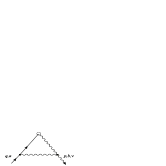
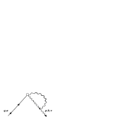
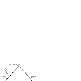
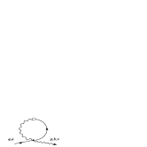
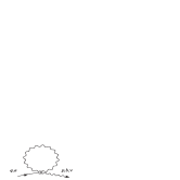
Figure 1: Diagrams contributing for the supercurrent and the gauge fixing term. The grey blob correspond to the operator insertion in which flows a momentum $(p-q)$.

In Fourier transformation (FT) we choose $p$ as the outcoming momemtun for the gluon field $A_{\mu}$ and $q$ the incoming momentum for the fermion field $\lambda$ (see Fig. 1). Each matrix element can be written as

$$\big{<}A_{\nu}^{b}(y)\,\bar{\lambda}^{a}(z)\,C(x)\big{>}\stackrel{{\scriptstyle FT}}{{\Longrightarrow}}D_{F}(q)\cdot(C(p,q))_{amp}\cdot D_{B}(p)\cdot\delta_{ab}\,,$$ (32)

where $(C(p,q))_{amp}$ can be, i.e., $\nabla_{\mu}S_{\mu}$, $\nabla_{\mu}T_{\mu}$, etc., with the external propagators amputated, $D_{F}(q)$ and $D_{B}(p)$ are the full fermion and gluon propagators, respectively, while $\delta_{ab}$ is the color structure, similar to all diagrams. The non-trivial part of the calculation is the determination of $(C(p,q))_{amp}$ for each matrix element in Eq. (27). $\big{<}{\cal O}\chi(x)\big{>}$, is not considered as we set the renormalized gluino mass to zero.

In order to determine $Z_{T}$ one should pick up from each matrix element of Eq. (27) those terms which contains the same Lorentz structure as $S_{\mu}$ and $T_{\mu}$, to tree-level. Those operators which do not contain the same tree-level Lorentz structure than $S_{\mu}$ and $T_{\mu}$ do not enter in the determination of $Z_{T}$. Below, we present the tree-level values of the different operator of Eq. (27). The calculation is straighforward.

For the case of the supercurrent (19), the tree-level part reads

$$S_{\mu}^{(0)}(x)=-\frac{2i}{g}\,\mbox{Tr}\,\bigg{\{}(\partial_{\rho}A_{\tau}(x)-\partial_{\tau}A_{\rho}(x))\sigma_{\rho\tau}\gamma_{\mu}\lambda(x)\bigg{\}}\,.$$ (33)

Using $\mbox{Tr}(T^{a}T^{b})=\frac{1}{2}\delta_{ab}$ for the traces and the antisymmetry of $\sigma_{\rho\tau}$ this expression becomes

$$S_{\mu}^{(0)}(x)=-2\delta_{ab}\partial_{\rho}A_{\tau}^{b}(x)\sigma_{\rho\tau}\gamma_{\mu}\lambda^{a}(x)\,.$$ (34)

or in FT,

$$\tilde{S}_{\mu}^{(0)}(r) = \int d^{4}xe^{ir\cdot x}S_{\mu}^{(0)}(x)$$ (35)

$$= -2i\delta_{ab}\sigma_{\rho\tau}\gamma_{\mu}\int d^{4}x\int\frac{d^{4}p}{(2\pi)^{4}}\int\frac{d^{4}q}{(2\pi)^{4}}\times$$

$$\times e^{i(r-p+q)x}p_{\rho}\tilde{A}_{\tau}^{b}(p)\tilde{\lambda}^{a}(q)$$

$$= -2i\delta_{ab}\sigma_{\rho\tau}\gamma_{\mu}\int\frac{d^{4}p}{(2\pi)^{4}}\int\frac{d^{4}q}{(2\pi)^{4}}\times$$

$$\times\delta(r-p+q)p_{\rho}\tilde{A}_{\tau}^{b}(p)\tilde{\lambda}^{a}(q)\,,$$

so we can define the vertex

$$\tilde{S}^{ab}_{\mu,\tau}(p,q)=-2i\delta_{ab}\sigma_{\rho\tau}\gamma_{\mu}p_{\rho}\,.$$ (36)

Concerning the operator $T_{\mu}$ in Eq. (23), the tree-level is

$$T_{\mu}^{(0)}(x)=i\delta_{ab}(\partial_{\mu}A_{\tau}^{b}(x)-\partial_{\tau}A_{\mu}^{b}(x))\gamma_{\tau}\lambda^{a}(x)$$ (37)

after the FT, we define the corresponding tree-level vertex,

$$\tilde{T}^{ab}_{\mu,\tau}(p,q)=\delta_{ab}(\not p\delta_{\mu\tau}-p_{\mu}\gamma_{\tau})\,.$$ (38)

The tree-level expression for the amputated matrix element $\big{<}{\cal O}\nabla_{\mu}S_{\mu}(x)\big{>}$ (using the notation in Eq. (32) is

$$\bigg{(}\nabla_{\mu}S_{\mu}\bigg{)}^{(0)}_{amp}\stackrel{{\scriptstyle FT}}{{\Longrightarrow}}2(p-q)_{\mu}\sigma_{\rho\nu}\gamma_{\mu}p_{\rho}\,,$$ (39)

while the tree-level expression for the amputated matrix element $\big{<}{\cal O}\nabla_{\mu}T_{\mu}(x)\big{>}$ is

$$\bigg{(}\nabla_{\mu}T_{\mu}\bigg{)}^{(0)}_{amp}\stackrel{{\scriptstyle FT}}{{\Longrightarrow}}i(\not pp_{\nu}-p^{2}\gamma_{\nu}-\not pq_{\nu}+p\cdot q\gamma_{\nu})\,.$$ (40)

In our convention, $\nabla_{\mu}=i(p-q)_{\mu}$, is the momentum transfer of the operator insertion.

From Eqs. (39,40) it is easy to see that, for $p=q$, a condition which would greatly simplify the calculation because implies that the operator insertion is at zero momentum, $\bigg{(}\nabla_{\mu}S_{\mu}(x)\bigg{)}^{(0)}_{amp}=\bigg{(}\nabla_{\mu}T_{\mu}(x)\bigg{)}^{(0)}_{amp}=0$. So the tree-level of $\nabla_{\mu}S_{\mu}$ and $\nabla_{\mu}T_{\mu}$ can not be distinguished at zero momentum transfer. In order to determine $Z_{T}$, different tree-level values of $S_{\mu}$ and $T_{\mu}$ are needed. To differenciate these tree-level values, general external momenta, $p$ and $q$ are required.

The value of the projections over $\gamma_{\alpha}$ and $\gamma_{\alpha}\gamma_{5}$ for the different matrix elements in Eq. (27) has been performed. Denoting $\frac{1}{4}\mbox{tr}(\gamma_{\alpha}(\nabla_{\mu}S_{\mu})_{amp})$ the projection over $\gamma_{\alpha}$ and $\frac{1}{4}\mbox{tr}(\gamma_{\alpha}\gamma_{5}(\nabla_{\mu}S_{\mu})_{amp})$ the projection over $\gamma_{\alpha}\gamma_{5}$ (tr is the trace over the gamma matrices which should not be confused with Tr, the trace over the color indices), it is easy to demonstrate that

$$\frac{1}{4}\mbox{tr}\bigg{(}\gamma_{\alpha}\bigg{(}\nabla_{\mu}S_{\mu}\bigg{)}^{(0)}_{amp}\bigg{)}\stackrel{{\scriptstyle FT}}{{\Longrightarrow}}$$

$$2i(p_{\alpha}p_{\nu}-p_{\alpha}q_{\nu}-p^{2}\delta_{\alpha\nu}+p\cdot q\delta_{\alpha\nu})$$ (41)

where $\frac{1}{4}\mbox{tr}(\gamma_{\mu}\gamma_{\rho})=\delta_{\mu\rho}$ and $\frac{1}{4}\mbox{tr}(\gamma_{5}\gamma_{\mu}\gamma_{\nu}\gamma_{\rho}\gamma_{\sigma})=\varepsilon_{\mu\nu\rho\sigma}$, while

$$\frac{1}{4}\mbox{tr}\bigg{(}\gamma_{\alpha}\gamma_{5}\bigg{(}\nabla_{\mu}S_{\mu}\bigg{)}^{(0)}_{amp}\bigg{)}\stackrel{{\scriptstyle FT}}{{\Longrightarrow}}2ip_{\rho}q_{\sigma}\varepsilon_{\nu\alpha\rho\sigma}\,.$$ (42)

Also

$$\frac{1}{4}\mbox{tr}\bigg{(}\gamma_{\alpha}\bigg{(}\nabla_{\mu}T_{\mu}\bigg{)}^{(0)}_{amp}\bigg{)}\stackrel{{\scriptstyle FT}}{{\Longrightarrow}}$$

$$i(p_{\alpha}p_{\nu}-p_{\alpha}q_{\nu}-p^{2}\delta_{\alpha\nu}+p\cdot q\delta_{\alpha\nu})$$ (43)

and

$$\frac{1}{4}\mbox{tr}\bigg{(}\gamma_{\alpha}\gamma_{5}\bigg{(}\nabla_{\mu}T_{\mu}\bigg{)}^{(0)}_{amp}\bigg{)}\stackrel{{\scriptstyle FT}}{{\Longrightarrow}}0\,.$$ (44)

Concerning the gauge fixing term, the tree-level value can be read from Eq. (83)

$$-\bigg{(}\frac{\delta S_{GF}}{\delta\xi(x)}|_{\xi=0}\bigg{)}^{(0)}_{amp}\stackrel{{\scriptstyle FT}}{{\Longrightarrow}}-2i\not pp_{\nu}$$ (45)

and the projections are

$$-\frac{1}{4}\mbox{tr}\bigg{(}\gamma_{\alpha}\bigg{(}\frac{\delta S_{GF}}{\delta\xi(x)}|_{\xi=0}\bigg{)}^{(0)}_{amp}\bigg{)}\stackrel{{\scriptstyle FT}}{{\Longrightarrow}}-2ip_{\alpha}p_{\nu}$$ (46)

and

$$-\frac{1}{4}\mbox{tr}\bigg{(}\gamma_{\alpha}\gamma_{5}\bigg{(}\frac{\delta S_{GF}}{\delta\xi(x)}|_{\xi=0}\bigg{)}^{(0)}_{amp}\bigg{)}\stackrel{{\scriptstyle FT}}{{\Longrightarrow}}0\,.$$ (47)

For the contact terms, the tree-level can be seen directly from Eq. (76) (with $a\to 0$)

$$\bigg{<}\frac{\delta{\cal O}}{\delta\xi(x)}|_{\xi=0}\bigg{>}^{(0)} = 2i\delta(x-y)\gamma_{\nu}\big{<}\lambda^{a}(y)\bar{\lambda}^{b}(z)\big{>}+$$ (48)

$$\delta(x-y)\big{<}A_{\nu}^{a}(y)\sigma_{\rho\tau}{\cal G}_{\rho\tau}^{b}(z)\big{>}$$

or in FT (in the limit $m_{0}\to 0$)

$$2i\gamma_{\nu}\bigg{(}\frac{1}{i\not q}\bigg{)}\delta_{ab}-2ip_{\rho}\frac{1}{p^{2}}\sigma_{\rho\nu}\delta_{ab}\,.$$ (49)

The projections are

$$\frac{1}{4}\mbox{tr}\bigg{(}\gamma_{\alpha}\bigg{(}\frac{\delta{\cal O}}{\delta\xi(x)}|_{\xi=0}\bigg{)}^{(0)}_{amp}\bigg{)}\stackrel{{\scriptstyle FT}}{{\Longrightarrow}}$$

$$2i(p_{\alpha}q_{\nu}-p\cdot q\delta_{\nu\alpha}+p^{2}\delta_{\alpha\nu})$$ (50)

and

$$\frac{1}{4}\mbox{tr}\bigg{(}\gamma_{\alpha}\gamma_{5}\bigg{(}\frac{\delta{\cal O}}{\delta\xi(x)}|_{\xi=0}\bigg{)}^{(0)}_{amp}\bigg{)}\stackrel{{\scriptstyle FT}}{{\Longrightarrow}}-2ip_{\rho}q_{\sigma}\varepsilon_{\nu\alpha\rho\sigma}\,.$$ (51)

Finally, the tree-level vertex for the operator in Eq. (25) is

$$(\tilde{B}_{0})^{ab}_{\tau}(p,q)=i\delta_{ab}(p_{\rho}p_{\tau}-p^{2}\delta_{\rho\tau})\gamma_{\rho}$$ (52)

while the projection is

$$\frac{1}{4}\mbox{tr}\bigg{(}\gamma_{\alpha}\big{(}B_{0}\big{)}^{(0)}_{amp}\bigg{)}\stackrel{{\scriptstyle FT}}{{\Longrightarrow}}i(p_{\alpha}p_{\nu}-p^{2}\delta_{\alpha\nu})\,.$$ (53)

For the operators in Eq. (26) we have

$$\frac{1}{4}\mbox{tr}(\gamma_{\alpha}(B_{1})_{amp})\stackrel{{\scriptstyle FT}}{{\Longrightarrow}}ip_{\nu}q_{\alpha}\,,$$

$$\frac{1}{4}\mbox{tr}(\gamma_{\alpha}(B_{2})_{amp})\stackrel{{\scriptstyle FT}}{{\Longrightarrow}}iq_{\nu}q_{\alpha}\,,$$

$$\frac{1}{4}\mbox{tr}(\gamma_{\alpha}(B_{3})_{amp})\stackrel{{\scriptstyle FT}}{{\Longrightarrow}}iq^{2}\delta_{\alpha\nu}$$ (54)

and

$$\frac{1}{4}\mbox{tr}\bigg{(}\gamma_{\alpha}\gamma_{5}\big{(}B_{0,1,2,3}\big{)}^{(0)}_{amp}\bigg{)}\stackrel{{\scriptstyle FT}}{{\Longrightarrow}}0\,.$$ (55)

The renormalization constants can be written as a power of $g_{0}$

$$Z_{operator}=Z_{operator}^{(0)}+g_{0}^{2}Z_{operator}^{(2)}+\cdots\,,$$ (56)

and also for the operators, a similar expansion can be done it

$$\big{<}Operator\big{>}=\big{<}Operator\big{>}^{(0)}+g_{0}^{2}\big{<}Operator\big{>}^{(2)}+\cdots\,,$$ (57)

where $\big{<}Operator\big{>}^{(2)}$, is the 1-loop correction while $\big{<}Operator\big{>}^{(0)}$, is the tree-level value.

Substituting Eq. (56) and Eq. (57) into Eq. (27), to order $g_{0}^{2}$, we obtain

$$(1+g_{0}^{2}Z_{S}^{(2)})\bigg{(}\big{<}{\cal O}\nabla_{\mu}S_{\mu}(x)\big{>}^{(0)}+$$

$$\hskip 85.35826ptg_{0}^{2}\big{<}{\cal O}\nabla_{\mu}S_{\mu}(x)\big{>}^{(2)}\bigg{)}+$$

$$g_{0}^{2}Z_{T}^{(2)}\big{<}{\cal O}\nabla_{\mu}T_{\mu}(x)\big{>}^{(0)}+$$

$$(1+g_{0}^{2}Z_{CT}^{(2)})\bigg{(}\bigg{<}\frac{\delta{\cal O}}{\delta\bar{\xi}(x)}|_{\xi=0}\bigg{>}^{(0)}+$$

$$\hskip 85.35826ptg_{0}^{2}\bigg{<}\frac{\delta{\cal O}}{\delta\bar{\xi}(x)}|_{\xi=0}\bigg{>}^{(2)}\bigg{)}-$$

$$(1+g_{0}^{2}Z_{GF}^{(2)})\bigg{(}\bigg{<}{\cal O}\,\frac{\delta S_{GF}}{\delta\bar{\xi}(x)}|_{\xi=0}\bigg{>}^{(0)}+$$

$$\hskip 85.35826ptg_{0}^{2}\bigg{<}{\cal O}\,\frac{\delta S_{GF}}{\delta\bar{\xi}(x)}|_{\xi=0}\bigg{>}^{(2)}\bigg{)}-$$

$$g_{0}^{2}Z_{FP}^{(2)}\bigg{<}{\cal O}\,\frac{\delta S_{FP}}{\delta\bar{\xi}(x)}|_{\xi=0}\bigg{>}^{(0)}+$$

$$g_{0}^{2}\sum_{j}Z_{B_{j}}^{(2)}\big{<}{\cal O}B_{j}(x)\big{>}^{(0)}=0$$ (58)

At tree-level we have, $Z_{S}^{(0)}=1,Z_{T}^{(0)}=0,Z_{CT}^{(0)}=1,Z_{GF}^{(0)}=1,Z_{FP}^{(0)}=0,Z_{B_{i}}^{(0)}=0$, so the lattice WTi is

$$\big{<}{\cal O}\nabla_{\mu}S_{\mu}(x)\big{>}^{(0)}+\bigg{<}\frac{\delta{\cal O}}{\delta\bar{\xi}(x)}|_{\xi=0}\bigg{>}^{(0)}-$$

$$\bigg{<}{\cal O}\,\frac{\delta S_{GF}}{\delta\bar{\xi}(x)}|_{\xi=0}\bigg{>}^{(0)}=0\,,$$ (59)

which holds in our lattice calculation. Eq. (59) was previously determined in the continuum galla2 . To order $g_{0}^{2}$ the lattice WTi is

$$\big{<}{\cal O}\nabla_{\mu}S_{\mu}(x)\big{>}^{(2)}+Z_{S}^{(2)}\big{<}{\cal O}\nabla_{\mu}S_{\mu}(x)\big{>}^{(0)}+$$

$$Z_{T}^{(2)}\big{<}{\cal O}\nabla_{\mu}T_{\mu}(x)\big{>}^{(0)}+$$

$$\bigg{<}\frac{\delta{\cal O}}{\delta\bar{\xi}(x)}|_{\xi=0}\bigg{>}^{(2)}+Z_{CT}^{(2)}\bigg{<}\frac{\delta{\cal O}}{\delta\bar{\xi}(x)}|_{\xi=0}\bigg{>}^{(0)}-$$

$$Z_{GF}^{(2)}\bigg{<}{\cal O}\,\frac{\delta S_{GF}}{\delta\bar{\xi}(x)}|_{\xi=0}\bigg{>}^{(0)}-\bigg{<}{\cal O}\,\frac{\delta S_{GF}}{\delta\bar{\xi}(x)}|_{\xi=0}\bigg{>}^{(2)}-$$

$$\sum_{j}Z_{B_{j}}^{(2)}\big{<}{\cal O}B_{j}(x)\big{>}^{(0)}=0\,.$$ (60)

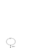
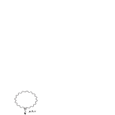
Figure 2: Non-zero diagrams contributing to the contact terms.

Notice that the Faddeev-Popov term $\bigg{<}{\cal O}\,\frac{\delta S_{FP}}{\delta\bar{\xi}(x)}|_{\xi=0}\bigg{>}^{(0)}$ in Eq. (58), is already $O(g_{0}^{2})$ (see Appendix B) and does not contribute to 1-loop order. In Fig. 1, the Feynman diagrams for $\big{<}{\cal O}\nabla_{\mu}S_{\mu}(x)\big{>}^{(2)}$ and $\bigg{<}{\cal O}\,\frac{\delta S_{GF}}{\delta\bar{\xi}(x)}|_{\xi=0}\bigg{>}^{(2)}$ are shown, while in Fig. 2, the non-zero contribution to contact terms are presented.

Let us substitute the tree-level values of the operators in Eq. (60) using the projections over $\gamma_{\alpha}$,

$$\frac{1}{4}\mbox{tr}\bigg{(}\gamma_{\alpha}\bigg{(}\nabla_{\mu}S_{\mu}\bigg{)}^{(2)}_{amp}\bigg{)}+$$

$$Z_{S}^{(2)}2i(p_{\alpha}p_{\nu}-p_{\alpha}q_{\nu}-p^{2}\delta_{\alpha\nu}+p\cdot q\delta_{\alpha\nu})+$$

$$Z_{T}^{(2)}i(p_{\alpha}p_{\nu}-p_{\alpha}q_{\nu}-p^{2}\delta_{\alpha\nu}+p\cdot q\delta_{\alpha\nu})+$$

$$\frac{1}{4}\mbox{tr}\bigg{(}\gamma_{\alpha}\bigg{(}\frac{\delta{\cal O}}{\delta\bar{\xi}(x)}|_{\xi=0}\bigg{)}_{amp}^{(2)}\bigg{)}+$$

$$Z_{CT}^{(2)}2i(p_{\alpha}q_{\nu}-p\cdot q\delta_{\alpha\nu}+p^{2}\delta_{\alpha\nu})-$$

$$Z_{GF}^{(2)}2ip_{\alpha}p_{\nu}-$$

$$\frac{1}{4}\mbox{tr}\bigg{(}\gamma_{\alpha}\bigg{(}\frac{\delta S_{GF}}{\delta\bar{\xi}(x)}|_{\xi=0}\bigg{)}_{amp}^{(2)}\bigg{)}+$$

$$\frac{1}{4}Z_{B_{j}}^{(2)}\mbox{tr}\big{<}\gamma_{\alpha}{\cal O}B_{j}\big{>}^{(0)}=0\,,$$ (61)

and the projections over $\gamma_{\alpha}\gamma_{5}$,

$$\frac{1}{4}\mbox{tr}\bigg{(}\gamma_{\alpha}\gamma_{5}\bigg{(}\nabla_{\mu}S_{\mu}\bigg{)}_{amp}^{(2)}\bigg{)}+$$

$$Z_{S}^{(2)}2ip_{\rho}q_{\sigma}\varepsilon_{\nu\alpha\rho\sigma}-$$

$$Z_{CT}^{(2)}2ip_{\rho}q_{\sigma}\varepsilon_{\nu\alpha\rho\sigma}+$$

$$\frac{1}{4}\mbox{tr}\bigg{(}\gamma_{\alpha}\gamma_{5}\bigg{(}\frac{\delta{\cal O}}{\delta\bar{\xi}(x)}|_{\xi=0}\bigg{)}_{amp}^{(2)}\bigg{)}-$$

$$\frac{1}{4}\mbox{tr}\bigg{(}\gamma_{\alpha}\gamma_{5}\bigg{(}\frac{\delta S_{GF}}{\delta\bar{\xi}(x)}|_{\xi=0}\bigg{)}_{amp}^{(2)}\bigg{)}+$$

$$\frac{1}{4}Z_{B_{j}}^{(2)}\mbox{tr}\big{<}\gamma_{\alpha}\gamma_{5}{\cal O}B_{j}\big{>}^{(0)}=0\,.$$ (62)

Our claim is that, in order to calculate $Z_{T}^{(2)}$ we can substitute $\frac{1}{4}Z_{B_{i}}^{(2)}\mbox{tr}\big{<}\gamma_{\alpha}{\cal O}B_{i}\big{>}^{(0)}\to Z_{B_{0}}^{(2)}i(p_{\alpha}p_{\nu}-p^{2}\delta_{\alpha\nu})+Z_{B_{1}}^{(2)}ip_{\nu}q_{\alpha}+Z_{B_{2}}^{(2)}iq_{\nu}q_{\alpha}+Z_{B_{3}}^{(2)}iq^{2}\delta_{\alpha\nu}$, and $\frac{1}{4}Z_{B_{i}}^{(2)}\mbox{Tr}\big{<}\gamma_{\alpha}\gamma_{5}{\cal O}B_{j}\big{>}^{(0)}\to 0$, where $Z_{B_{j}}$ correspond to the renormalization constant in Eq. (53,54,55). No other $Z_{B_{j}}$ are needed, because there are no other $B_{j}$’s that would contribute with the same Lorentz structures appearing in the tree-level of Eqs. (61,62).

Each matrix element in Eqs. (61,62) has been calculated for general $p$ and $q$ (off-shell regime). To deal with the IR divergencies and rinormalize to 1-loop order the Kawai procedure is used kawai , with the help of tabulated results in martinelli ; haris . Once $p$ and $q$ have been extracted from the propagators through the Kawai procedure, the rest of the integral depend on the loop momenta which is numerically integrated. A similar renormalization procedure has been used to calculate the 3-loop beta function in QCD with Wilson fermions feo6 and the 3-loop free-energy in QCD with Wilson fermions feo7 ; feo8 (for a complete study of the off-shell WTi in QCD see menotti ). Tipically, each matrix element contains $\approx 1000$ terms (in particular dilogarithms functions depending on both external momenta which coming from the diagrams with three propagators in Fig. 1). After the numerical integration, one can simplify the results in order to read the value of $Z_{T}$ by setting

$$p^{2}=q^{2}\,\,\,\,\mbox{and}\,\,\,\,p\cdot q=0\,,$$ (63)

(see Appendix C). This is still an off-shell condition (because even if $p^{2}=q^{2}$, there are no other condition on this expression, i.e., $q^{2}=0$), but drastically reduces the number and difficulty of the expressions (for example, the dilogarithm terms simplify).

Let us introduce, for simplicity, the notation, $\Delta\equiv{\cal O}\nabla_{\mu}S_{\mu}(x)+\frac{\delta{\cal O}}{\delta\bar{\xi}(x)}|_{\xi=0}-{\cal O}\,\frac{\delta S_{GF}}{\delta\bar{\xi}(x)}|_{\xi=0}$. Using Eq. (63), we get the following dependence on $p$ and $q$ for $\mbox{tr}\big{<}\gamma_{\alpha}\Delta\big{>}^{(2)}$ and $\mbox{tr}\big{<}\gamma_{\alpha}\gamma_{5}\Delta\big{>}^{(2)}$,

$$\mbox{tr}\big{<}\gamma_{\alpha}\Delta\big{>}^{(2)} \stackrel{{\scriptstyle FT}}{{\Longrightarrow}} A_{1}q^{2}\hat{p}_{\alpha}\hat{p}_{\nu}+A_{2}q^{2}\hat{p}_{\alpha}\hat{q}_{\nu}+$$ (64)

$$(A_{3}+M_{3})q^{2}\delta_{\alpha\nu}+M_{1}q^{2}\hat{p}_{\nu}\hat{q}_{\alpha}+M_{2}q^{2}\hat{q}_{\alpha}\hat{q}_{\nu}+$$

$$P_{1}q^{2}\hat{p}_{\nu}^{2}\delta_{\nu\alpha}+P_{2}q^{2}\hat{q}_{\nu}^{2}\delta_{\nu\alpha}+\cdots$$

and

$$\mbox{tr}\big{<}\gamma_{\alpha}\gamma_{5}\Delta\big{>}^{(2)}\stackrel{{\scriptstyle FT}}{{\Longrightarrow}}A_{4}q^{2}\hat{p}_{\rho}\hat{q}_{\sigma}\varepsilon_{\nu\alpha\rho\sigma}\,,$$ (65)

where the dots in Eq. (64) indicate that because the semplification in Eq. (63) is used, some momenta dependence are missing or mixed with others, i.e., $p\cdot q\delta_{\nu\alpha}$ does not appear, while $p^{2}\delta_{\nu\alpha}$, is mixed with $q^{2}\delta_{\nu\alpha}$, (see Appendix C for notation).

It is also interesting to see the Lorentz structure of the supercurrent,

$$\mbox{tr}\big{<}\gamma_{\alpha}S_{\mu}\big{>}^{(2)} \stackrel{{\scriptstyle FT}}{{\Longrightarrow}} N_{1}q\,\hat{p}_{\mu}\hat{p}_{\nu}\hat{p}_{\alpha}+N_{2}q\,\hat{q}_{\mu}\hat{p}_{\nu}\hat{p}_{\alpha}+$$ (66)

$$N_{3}q\,\hat{p}_{\mu}\hat{q}_{\nu}\hat{p}_{\alpha}+N_{4}q\,\hat{q}_{\mu}\hat{q}_{\nu}\hat{p}_{\alpha}+N_{5}q\,\hat{p}_{\mu}\hat{p}_{\nu}\hat{q}_{\alpha}+$$

$$N_{6}q\,\hat{q}_{\mu}\hat{p}_{\nu}\hat{q}_{\alpha}+N_{7}q\,\hat{p}_{\mu}\hat{q}_{\nu}\hat{q}_{\alpha}+N_{8}q\,\hat{q}_{\mu}\hat{q}_{\nu}\hat{q}_{\alpha}+$$

$$Q_{1}q\,\hat{p}_{\alpha}\delta_{\mu\nu}+Q_{2}q\,\hat{q}_{\alpha}\delta_{\mu\nu}+Q_{3}q\,\hat{p}_{\nu}\delta_{\mu\alpha}+$$

$$Q_{4}q\,\hat{q}_{\nu}\delta_{\mu\alpha}+Q_{5}q\,\hat{p}_{\mu}\delta_{\nu\alpha}+Q_{6}q\,\hat{q}_{\mu}\delta_{\nu\alpha}+$$

$$R_{1}q\,\hat{p}_{\mu}\delta_{\mu\nu\alpha}+R_{2}q\,\hat{q}_{\mu}\delta_{\mu\nu\alpha}+\cdots$$

where the coefficient $A_{i},M_{j},Q_{k}$, are tipically of the form

$$(C_{n}+C_{m}\mbox{Ln}(a^{2}q^{2}))$$ (67)

while $P_{i},N_{j},R_{k}$, do not contain $\mbox{Ln}(a^{2}q^{2})$ terms. Here, $C_{n}$ are lattice constants or numbers coming from the numerical integration and $C_{m}$ are rational numbers coming from the Kawai procedure. Notice that the Lorentz structures multiplying $P_{i},R_{k}$ in Eq. (64,66) are non-Lorentz covariant, even in the continuum limit $(a\to 0)$.

From Eqs. (61,62,64,65) the following conditions can be derived

$$A_{1}=-2iZ_{S}^{(2)}-iZ_{T}^{(2)}+2iZ_{GF}^{(2)}-iZ_{B_{0}}^{(2)}\,,$$

$$A_{3}+M_{3}=2iZ_{S}^{(2)}+iZ_{T}^{(2)}-2iZ_{CT}^{(2)}+iZ_{B_{0}}^{(2)}-iZ_{B_{3}}^{(2)}\,,$$

$$M_{1}=-iZ_{B_{1}}^{(2)}\,,$$

$$M_{2}=-iZ_{B_{2}}^{(2)}\,$$ (68)

and

$$A_{2}=2iZ_{S}^{(2)}+iZ_{T}^{(2)}-2iZ_{CT}^{(2)}\,,$$

$$A_{4}=-2iZ_{S}^{(2)}+2iZ_{CT}^{(2)}\,.$$ (69)

The last two conditions can be explicitly solved for $Z_{T}^{(2)}$,

$$Z_{T}^{(2)}=-iA_{2}-iA_{4}\,.$$ (70)

Eq. (70) is the only possible solution of the system (61,62) for $Z_{T}^{(2)}$. Our result is $Z_{T}^{(2)}|_{1-loop}=0.664$. A VEGAS Monte Carlo routine to perform the 1 loop integration with 200 millions of points, using the GNU Scientific Library is used. To estimate the error we take the value given by the program which is $\approx 10^{-5}$ for each integral. The calculation, once $p$ and $q$ has been extracted from the propagators, involves around 1300 different 1-loop integrals. For each diagram tipically we have 100 different integrals. That means that the error is around $10^{-3}$.

Let us compare our perturbative result with the numerical one farchioni , $Z_{T}^{NUM}\equiv Z_{T}/Z_{S}=0.185(7)$. One has to observe that the definition used here for $S_{\mu}$ is not the same as in farchioni . It is easy to demonstrate that $Z_{T}^{NUM}=\frac{1}{2}Z_{T}^{PT}$ farchioni2 . To compare with the numerical results one as to divide the perturbative value by 2 which gives, $Z_{T}^{PT}=\frac{1}{2}Z_{T}^{(2)}|_{1-loop}=0.332$. We are currently increasing the precision of the numerical integration to 400 milion of points. A detailed presentation of the results in Eqs. (64,65) together with the result of each diagram is under way feo3 .

V Discussion and conclusions

In this paper, the SUSY WTi in 1-loop LPT has been investigated. A general procedure in order to get the renormalization constant for the supercurrent has been presented. In LPT it is possible to determine the value of the renormalization constant for the supercurrent from the off-shell regime of the SUSY WTi. The computation of each matrix elements of the WTi has been carried out using the symbolic language Mathematica. The programs were completely wroted by the author together with the numerical code used for the integration. All the contributions have been calculated in the off-shell regime, and in order to get the value of the renormalization constant, a simplification in the external momenta (which still keeps the off-shell regime) has been applyed. We are currently increasing the precision of the numerical integration and a detailed presentation of the results is the subject of a forthcoming paper feo3 . A reasonable good agreement of our perturbative result for the renormalization constant, $Z_{T}^{PT}=0.332$, in comparison with the numerical one, $Z_{T}^{NUM}=0.185(7)$, has been achieved, taking in consideration the fact that in the numerical simulation $g_{0}^{2}=4/2.3$, which still corresponds to the non-perturbative region. We observe that, at least at 1-loop order in perturbation theory, $Z_{T}$ is finite. This result may have some theoretical implications which we are currently investigating. Also, the determination of $Z_{S}$, using another kind of gamma projections is under investigation. It would be interesting to calculate $Z_{S}$ in order to check the trace anomaly and the exact renormalization expression for Eq. (29). An important point to stress here is that, even in the continuum limit, we observe in Eq. (64) Lorentz breaking terms which coming from the fact that we substituted $X_{S}$ by the Eq. (24). It would be interesting to see whether Eq. (64) is the continuum off-shell WTi. The nice point is that, once the $Z_{T}$ has been determined, we can impose the on-shell condition on the gluino mass. The Lorentz breaking terms cancel out from Eq. (64) and the continuum WTi is recovered. At least to 1-loop order, we do not observe a SUSY anomaly in $N=1$ SYM, altough a more carefully study is required.

Appendix A Perturbative Calculation

In this appendix we follow the lines of feo ; galla2 . The lattice SUSY transformations of the gauge field $A_{\mu}(x)$ are not equal to the continuum ones. On the lattice the transformation of the gauge link $U_{\mu}(x)$ determines the transformation properties of $A_{\mu}(x)$. Writing the link variable as

$$U_{\mu}(x)=e^{-aA_{\mu}\left(x+\frac{a}{2}\hat{\mu}\right)}\,,$$ (71)

for the SUSY transformations of the gauge link we use the symmetric choice galla

$$\delta U_{\mu}(x) = -ag_{0}U_{\mu}(x)\bar{\xi}(x)\gamma_{\mu}\lambda(x)$$

$$-ag_{0}\bar{\xi}(x+a\hat{\mu})\gamma_{\mu}\lambda(x+a\hat{\mu})U_{\mu}(x)\,.$$

These two equations determine the transformation behavior of the field $A_{\mu}(x)$ feo . The FT for the gauge field is defined as the usual way

$$A^{b}_{\mu}(x)=\int d^{4}k\tilde{A}^{b}_{\mu}(k)e^{ik\cdot(x+\frac{a}{2}\hat{\mu})}\,.$$ (72)

Collecting all terms until order $g_{0}^{2}$ we can write down the variation of the gauge field $A_{\mu}^{b}(x)$ as feo

$$\delta A_{\mu}^{b}(x) = i\bigg{(}\bar{\xi}(x)\gamma_{\mu}\lambda^{b}(x)+\bar{\xi}(x+a\hat{\mu})\gamma_{\mu}\lambda^{b}(x+a\hat{\mu})\bigg{)}+$$ (73)

$$\frac{i}{2}ag_{0}f_{abc}\bigg{(}\bar{\xi}(x)\gamma_{\mu}\lambda^{c}(x)-\bar{\xi}(x+a\hat{\mu})\gamma_{\mu}\lambda^{c}(x+a\hat{\mu})\bigg{)}A_{\mu}^{a}-$$

$$\frac{i}{24}a^{2}g_{0}^{2}\bigg{(}2\delta_{ab}\delta_{cd}-\delta_{ac}\delta_{bd}-\delta_{ad}\delta_{bc}\bigg{)}A_{\mu}^{c}A_{\mu}^{d}\times$$

$$\times\bigg{(}\bar{\xi}(x)\gamma_{\mu}\lambda^{a}(x)+\bar{\xi}(x+a\hat{\mu})\gamma_{\mu}\lambda^{a}(x+a\hat{\mu})\bigg{)}$$

which reduces to the continuum SUSY transformation $\delta A_{\mu}^{a}(x)=2i\bar{\xi}\gamma_{\mu}\lambda^{a}(x)$ in the continuum limit $a\rightarrow 0$. Because in this paper we fix $N_{c}=2$, some semplifications appear

$$\mbox{Tr}\bigg{\{}T^{a}T^{b}T^{c}T^{d}\bigg{\}} = \frac{1}{8}(\delta_{ab}\delta_{cd}-f_{abe}f_{cde})\,,$$

$$f_{abe}f_{cde} = (\delta_{ac}\delta_{bd}-\delta_{ad}\delta_{bc})\,.$$ (74)

Using the Eq. (73), it is possible to determine the differents pieces of the WTi in Eq. (27), i.e., the contact terms, the gauge fixing term and the Faddeev-Popov term. They are necessary in order to calculate the Feynman rules for 1-loop order calculation. In appendix B, the vertices coming from these pieces are presented together with the ones coming from the supercurrent.

Appendix B Vertices

Let us determine the contact terms, $\frac{\delta{\cal O}}{\delta\bar{\xi}(x)}|_{\xi=0}$. First of all, the variation of the operator insertion, ${\cal O}=A_{\nu}^{a}(y)\bar{\lambda}^{b}(z)$, is

$$\delta{\cal O}=\delta A_{\nu}^{a}(y)\bar{\lambda}^{b}(z)+A_{\nu}^{a}(y)\delta\bar{\lambda}^{b}(z)\,.$$ (75)

Substituting (73) into (75), after some algebra, we obtain

$$\bigg{<}\frac{\delta{\cal O}}{\delta\bar{\xi}(x)}|_{\xi=0}\bigg{>}=$$

$$=i\delta(x-y)\gamma_{\nu}\bigg{<}\lambda^{a}(y)\bar{\lambda}^{b}(z)\bigg{>}+$$

$$i\delta(x-y-a\hat{\nu})\gamma_{\nu}\bigg{<}\lambda^{a}(y+a\hat{\nu})\bar{\lambda}^{b}(z)\bigg{>}+$$

$$\frac{i}{2}ag_{0}f_{dac}\delta(x-y)\gamma_{\nu}\bigg{<}\lambda^{c}(y)A_{\nu}^{d}(y)\bar{\lambda}^{b}(z)\bigg{>}-$$

$$\frac{i}{2}ag_{0}f_{dac}\delta(x-y-a\hat{\nu})\gamma_{\nu}\bigg{<}\lambda^{c}(y+a\hat{\nu})A_{\nu}^{d}(y)\bar{\lambda}^{b}(z)\bigg{>}-$$

$$\frac{i}{24}a^{2}g_{0}^{2}\bigg{(}2\delta_{ae}\delta_{cd}-\delta_{ec}\delta_{ad}-\delta_{ed}\delta_{ac}\bigg{)}\delta(x-y)\times$$

$$\hskip 25.6073pt\times\bigg{<}A_{\nu}^{c}(y)A_{\nu}^{d}(y)\lambda^{e}(y)\bar{\lambda}^{b}(z)\bigg{>}$$

$$-\frac{i}{24}a^{2}g_{0}^{2}\bigg{(}2\delta_{ae}\delta_{cd}-\delta_{ec}\delta_{ad}-\delta_{ed}\delta_{ac}\bigg{)}\delta(x-y-a\hat{\nu})\times$$

$$\hskip 25.6073pt\times\bigg{<}A_{\nu}^{c}(y)A_{\nu}^{d}(y)\lambda^{e}(y+a\hat{\nu})\bar{\lambda}^{b}(z)\bigg{>}+$$

$$\delta(x-y)\bigg{<}A_{\nu}^{a}(y)\sigma_{\rho\tau}{\cal G}_{\rho\tau}^{b}(z)\bigg{>}\,,$$ (76)

where ${\cal G}_{\rho\tau}(z)=-ig_{0}{\cal G}_{\rho\tau}^{b}(z)T^{b}$.

The part of the lattice action corresponding to the gauge fixing is defined as

$$S_{GF} = \frac{a^{2}}{2}\sum_{x}\bigg{(}\sum_{\rho}(A_{\rho}^{c}(x)-A_{\rho}^{c}(x-a\hat{\rho}))\bigg{)}^{2}$$

$$=\frac{a^{4}}{2}\sum_{x}\bigg{(}\sum_{\rho}\nabla_{\rho}^{back}A_{\rho}^{c}(x)\bigg{)}^{2}$$

$$=\frac{a^{4}}{2}\sum_{x}\bigg{(}\sum_{\rho}\nabla_{\rho}^{back}A_{\rho}^{c}(x)\bigg{)}\bigg{(}\sum_{\tau}\nabla_{\tau}^{back}A_{\tau}^{c}(x)\bigg{)}$$

where $\nabla_{\rho}^{back}f(x)=\frac{1}{a}\,\bigg{(}f(x)-f(x-a\hat{\rho})\bigg{)}$. The variation of the gauge fixing term (B) can be written as

$$\delta S_{GF}=a^{4}\sum_{x}\bigg{(}\sum_{\rho}\nabla_{\rho}^{back}\delta A_{\rho}^{c}(x)\bigg{)}\bigg{(}\sum_{\tau}\nabla_{\tau}^{back}A_{\tau}^{c}(x)\bigg{)}\,.$$ (78)

This results in the contribution of the gauge fixing term into the WTi as

$$-\bigg{<}{\cal O}\,\frac{\delta S_{GF}}{\delta\xi(x)}|_{\xi=0}\bigg{>}=$$

$$i\gamma_{\rho}\bigg{[}\bigg{<}\lambda^{c}(x)\nabla_{\rho}^{forw}\nabla_{\tau}^{back}\bigg{(}A_{\tau}^{c}(x)+$$

$$\hskip 56.9055ptA_{\tau}^{c}(x-a\hat{\rho})\bigg{)}A_{\nu}^{a}(y)\bar{\lambda}^{b}(z)\bigg{>}+$$

$$\frac{i}{2}ag_{0}f_{ecf}\gamma_{\rho}\bigg{<}\lambda^{f}(x)\bigg{(}A_{\rho}^{e}\nabla_{\rho}^{forw}\nabla_{\tau}^{back}A_{\tau}^{c}(x)-$$

$$A_{\rho}^{e}(x-a\hat{\rho})\nabla_{\rho}^{forw}\nabla_{\tau}^{back}A_{\tau}^{c}(x-a\hat{\rho})\bigg{)}A_{\nu}^{a}(y)\bar{\lambda}^{b}(z)\bigg{>}-$$

$$\frac{i}{24}a^{2}g_{0}^{2}\gamma_{\rho}\bigg{(}2\delta_{ec}\delta_{fd}-\delta_{ef}\delta_{cd}-\delta_{ed}\delta_{fc}\bigg{)}\times$$

$$\hskip 56.9055pt\times\bigg{<}\lambda^{e}(x)\bigg{(}A_{\rho}^{f}A_{\rho}^{d}\nabla_{\rho}^{forw}\nabla_{\tau}^{back}A_{\tau}^{c}(x)+$$

$$A_{\rho}^{f}(x-a\hat{\rho})A_{\rho}^{d}(x-a\hat{\rho})\nabla_{\rho}^{forw}\nabla_{\tau}^{back}A_{\tau}^{c}(x-a\hat{\rho})\bigg{)}\times$$

$$\hskip 56.9055pt\times A_{\nu}^{a}(y)\bar{\lambda}^{b}(z)\bigg{>}\bigg{]}\,,$$ (79)

where $\nabla_{\rho}^{forw}f(x)=\frac{1}{a}\,\big{(}f(x-a\hat{\rho})-f(x)\big{)}$.

Finally, the expansion of the Faddeev Popov action can be written as

$$S_{FP} = a^{2}\sum_{x,\rho^{<}_{>}0}\bigg{[}\bar{\eta}^{a}(x)\bigg{(}\delta_{ab}+\frac{1}{2}ag_{0}A_{\rho}^{c}f^{acb}+$$ (80)

$$\frac{1}{12}a^{2}g_{0}^{2}A_{\rho}^{c}A_{\rho}^{d}f^{ace}f^{edb}\bigg{)}\eta^{b}(x)-$$

$$\bar{\eta}^{a}(x)\bigg{(}\delta_{ab}-\frac{1}{2}ag_{0}A_{\rho}^{c}f^{acb}+$$

$$\frac{1}{12}a^{2}g_{0}^{2}A_{\rho}^{c}A_{\rho}^{d}f^{ace}f^{edb}\bigg{)}\eta^{b}(x+a\hat{\rho})\bigg{]}$$

and the contribution of the Faddeev-Popov term into the WTi is

$$-\bigg{<}{\cal O}\,\frac{\delta S_{FP}}{\delta\bar{\xi}(x)}|_{\xi=0}\bigg{>}=$$

$$-\frac{ig_{0}}{2a}f^{gch}\sum_{\rho}\gamma_{\rho}\bigg{<}$$

$$\bigg{[}\bar{\eta}^{g}(x)\lambda^{c}(x)\bigg{(}\eta^{h}(x)+\eta^{h}(x+a\hat{\rho})\bigg{)}+$$

$$\bar{\eta}^{g}(x-a\hat{\rho})\lambda^{c}(x)\bigg{(}\eta^{h}(x-a\hat{\rho})+\eta^{h}(x)\bigg{)}-$$

$$\bar{\eta}^{g}(x+a\hat{\rho})\lambda^{c}(x)\bigg{(}\eta^{h}(x+a\hat{\rho})+\eta^{h}(x)\bigg{)}+$$

$$\bar{\eta}^{g}(x)\lambda^{c}(x)\bigg{(}\eta^{h}(x)+\eta^{h}(x-a\hat{\rho})\bigg{)}\bigg{]}A_{\nu}^{a}(y)\bar{\lambda}^{b}(z)\bigg{>}-$$

$$\frac{ig_{0}^{2}}{4}f^{gch}f^{dcf}\sum_{\rho}\gamma_{\rho}\bigg{<}$$

$$\bigg{[}\bar{\eta}^{g}(x)\lambda^{f}(x)A_{\rho}^{d}\bigg{(}\eta^{h}(x)+\eta^{h}(x+a\hat{\rho})\bigg{)}-$$

$$\bar{\eta}^{g}(x-a\hat{\rho})\lambda^{f}(x)A_{\rho}^{d}(x-a\hat{\rho})\bigg{(}\eta^{h}(x-a\hat{\rho})+\eta^{h}(x)\bigg{)}-$$

$$\bar{\eta}^{g}(x+a\hat{\rho})\lambda^{f}(x)A_{\rho}^{d}\bigg{(}\eta^{h}(x+a\hat{\rho})+\eta^{h}(x)\bigg{)}+$$

$$\bar{\eta}^{g}(x)\lambda^{f}(x)A_{\rho}^{d}(x-a\hat{\rho})\bigg{(}\eta^{h}(x)+\eta^{h}(x-a\hat{\rho})\bigg{)}\bigg{]}\times$$

$$\hskip 56.9055pt\times A_{\nu}^{a}(y)\bar{\lambda}^{b}(z)\bigg{>}-$$

$$\frac{ig_{0}^{2}}{12}f^{gce}f^{edh}\sum_{\rho}\gamma_{\rho}\bigg{<}$$

$$\bigg{[}\bar{\eta}^{g}(x)\bigg{(}\lambda^{c}(x)A_{\rho}^{d}+A_{\rho}^{c}\lambda^{d}(x)\bigg{)}\bigg{(}$$

$$\hskip 56.9055pt\eta^{h}(x)-\eta^{h}(x+a\hat{\rho})\bigg{)}+$$

$$\bar{\eta}^{g}(x-a\hat{\rho})\bigg{(}\lambda^{c}(x)A_{\rho}^{d}(x-a\hat{\rho})+$$

$$\hskip 45.52458ptA_{\rho}^{c}(x-a\hat{\rho})\lambda^{d}(x)\bigg{)}\bigg{(}\eta^{h}(x-a\hat{\rho})-\eta^{h}(x)\bigg{)}+$$

$$\bar{\eta}^{g}(x+a\hat{\rho})\bigg{(}\lambda^{c}(x)A_{\rho}^{d}(x)+A_{\rho}^{c}(x)\lambda^{d}(x)\bigg{)}\bigg{(}$$

$$\hskip 56.9055pt\eta^{h}(x+a\hat{\rho})-\eta^{h}(x)\bigg{)}+$$

$$\bar{\eta}^{g}(x)\bigg{(}\lambda^{c}(x)A_{\rho}^{d}(x-a\hat{\rho})+A_{\rho}^{c}(x-a\hat{\rho})\lambda^{d}(x)\bigg{)}\bigg{(}$$

$$\hskip 39.83368pt\eta^{h}(x)-\eta^{h}(x-a\hat{\rho})\bigg{)}\bigg{]}A_{\nu}^{a}(y)\bar{\lambda}^{b}(z)\bigg{>}\,,$$ (81)

where $A_{\rho}^{c}\equiv A_{\rho}^{c}(x+\frac{a\hat{\rho}}{2})$. It is possible to calculate the vertices and the corresponding Feynman diagrams, up to order $g_{0}^{2}$, from Eq. (76,79,81) in FT.

Regarding the contact terms in Eq. (76), all the contributions to order $g_{0}^{2}$ are zero except for the last line of Eq. (76). The corresponding non-zero Feynman diagrams are shown in Fig 2. The vertices used here are, the two-gluons vertex,

$$\tilde{G}_{2\tau\rho}^{abc}(k_{1},k_{2}) = -\frac{1}{2}g_{0}f_{abc}\bigg{\{}\sigma_{\rho\tau}\bigg{[}$$ (82)

$$\cos(\frac{k_{1\rho}a}{2}+\frac{k_{2\rho}a}{2})\cos(\frac{k_{1\rho}a}{2})\cos(\frac{k_{1\tau}a}{2}+k_{2\tau}a)+$$

$$\cos(\frac{k_{1\tau}a}{2}+\frac{k_{2\tau}a}{2})\cos(\frac{k_{2\tau}a}{2})\cos(\frac{k_{2\rho}a}{2}+k_{1\rho}a)-$$

$$\sin(\frac{k_{1\rho}a}{2}+\frac{k_{2\rho}a}{2})\sin(\frac{k_{1\rho}a}{2})\cos(\frac{k_{1\tau}a}{2})-$$

$$\sin(\frac{k_{1\tau}a}{2}+\frac{k_{2\tau}a}{2})\sin(\frac{k_{2\tau}a}{2})\cos(\frac{k_{2\rho}a}{2})\bigg{]}-$$

$$\delta_{\rho\tau}\sum_{\alpha}\sigma_{\alpha\tau}\sin(\frac{k_{1\tau}a}{2}+\frac{k_{2\tau}a}{2})\bigg{(}\sin(k_{1\alpha}a)-$$

$$\hskip 56.9055pt\sin(k_{2\alpha}a)\bigg{)}\bigg{\}}\,,$$

and the three-gluons vertex, which we do not reported here and gives a zero contrbution to the last diagram of Fig. 2.

For the gauge fixing terms in Eq. (79), we need the vertex with one-gluon-one-gluino (which is similar to Eq. (45) in the continuum limit,

$$\widetilde{GF}_{1\rho\tau}^{ab}(p,k)=-\frac{4i}{a^{2}}\delta_{ab}\gamma_{\rho}\sin(k_{\rho}a)\sin(\frac{k_{\tau}a}{2})\,,$$ (83)

the vertex with two-gluons-one-gluino

$$\widetilde{GF}_{2\tau\rho}^{fce}(p,q,k) =$$ (84)

$$\frac{2g_{0}}{a}f_{ecf}\bigg{\{}\gamma_{\rho}\sin(\frac{k_{\rho}a}{2}+\frac{q_{\rho}a}{2})\sin(\frac{q_{\rho}a}{2})\sin(\frac{q_{\tau}a}{2})-$$

$$\gamma_{\tau}\sin(\frac{k_{\tau}a}{2}+\frac{q_{\tau}a}{2})\sin(\frac{k_{\tau}a}{2})\sin(\frac{k_{\rho}a}{2})\bigg{\}}$$

and finally the three-gluons-one-gluino vertex (non-symmetrized)

$$\widetilde{GF}_{3\rho\sigma\tau}^{efdc}(p,k,q,t) =$$ (85)

$$-\frac{1}{3}g_{0}^{2}\bigg{(}2\delta_{ec}\delta_{fd}-\delta_{ef}\delta_{cd}-\delta_{ed}\delta_{fc}\bigg{)}\gamma_{\rho}\delta_{\rho\sigma}\times$$

$$\times\sin(\frac{k_{\rho}a}{2}+\frac{q_{\rho}a}{2}+\frac{t_{\rho}a}{2})\sin(\frac{t_{\rho}a}{2})\sin(\frac{t_{\tau}a}{2})\,.$$

For the Faddeev-Popov terms in Eq. (81), we need one-gluino-ghost-antighost vertex

$$\widetilde{FP}_{\rho}^{cgh}(p,-q,k) =$$ (86)

$$\frac{4g_{0}}{a}f^{gch}\sum_{\rho}\gamma_{\rho}\cos(\frac{k_{\rho}a}{2})\sin(\frac{q_{\rho}a}{2})\cos(\frac{k_{\rho}a}{2}-\frac{q_{\rho}a}{2})$$

and one-gluino-one-gluon-ghost-antighost vertex

$$\widetilde{FP}_{1\rho}^{cdgh}(p,t,-q,k) =$$ (87)

$$-\frac{2i}{3}g_{0}^{2}(f^{gce}f^{edh}+f^{gde}f^{ech})\gamma_{\rho}\bigg{\{}$$

$$\sin(\frac{k_{\rho}a}{2})\sin(\frac{q_{\rho}a}{2})\cos(\frac{k_{\rho}a}{2}+\frac{t_{\rho}a}{2}-\frac{q_{\rho}a}{2})\bigg{\}}\,.$$

As we can see from Eq. (86) and (87) the vertices are already order $g_{0}$ and $g_{0}^{2}$, so pluging into Eq (58) is already more than $O(g_{0}^{2})$. This imply that the Faddeev-Popov terms do not contribute to order $g_{0}^{2}$.

Concerning the vertices of $S_{\mu}$ for a 1-loop calculation we need the vertices corresponding to one-gluon-one-gluino, the two-gluons-one-gluino and finally the three-gluons-one gluino. They can be calculated from (19). The vertex one-gluon-one-gluino (using Eq. (35)) is

$$\tilde{S}_{1\mu,\rho\tau}^{abc}(q,p)=-\frac{2i}{a}\delta_{ab}\sigma_{\rho\tau}\gamma_{\mu}\cos(\frac{p_{\tau}a}{2})\sin(p_{\rho}a)\,,$$ (88)

which reduce to the continuum one in the limit $a\to 0$ (see Eq. (36)), while the vertex two-gluons-one-gluino is

$$\tilde{S}_{2\mu,\rho\tau}^{abc}(q,p_{1},p_{2}) = \frac{1}{2}g_{0}f_{abc}\bigg{\{}\sigma_{\rho\tau}\gamma_{\mu}\bigg{[}$$ (89)

$$\cos(\frac{p_{1\rho}a}{2}+\frac{p_{2\rho}a}{2})\cos(\frac{p_{1\rho}a}{2})\cos(\frac{p_{1\tau}a}{2}+p_{2\tau}a)+$$

$$\cos(\frac{p_{1\tau}a}{2}+\frac{p_{2\tau}a}{2})\cos(\frac{p_{2\tau}a}{2})\cos(\frac{p_{2\rho}a}{2}+p_{1\rho}a)-$$

$$\sin(\frac{p_{1\rho}a}{2}+\frac{p_{2\rho}a}{2})\sin(\frac{p_{1\rho}a}{2})\cos(\frac{p_{1\tau}a}{2})-$$

$$\sin(\frac{p_{1\tau}a}{2}+\frac{p_{2\tau}a}{2})\sin(\frac{p_{2\tau}a}{2})\cos(\frac{p_{2\rho}a}{2})\bigg{]}-$$

$$\delta_{\rho\tau}\sum_{\alpha}\sigma_{\alpha\tau}\gamma_{\mu}\sin(\frac{p_{1\tau}a}{2}+\frac{p_{2\tau}a}{2})\bigg{(}\sin(p_{1\alpha}a)-$$

$$\hskip 56.9055pt\sin(p_{2\alpha}a)\bigg{)}\bigg{\}}\,.$$

We do not presented here the three-gluons-one-gluino vertex because its contribution to the last Feynman diagram for the supercurrent, in Fig. 1, is zero by color considerations.

Appendix C Off-shell regime

In order to separate the contribution of $T_{\mu}$ and $S_{\mu}$ at tree-level, we can not impose $p=q$, that would greatly simplify the calculation. We are forced to use general external momenta $p$ and $q$ (while the momentum transfer of the operator insertion is $(p-q)\neq 0$, see Fig. 1). Once the external momenta has been extracted from the propagators, in order to get the value of $Z_{T}$, the semplification $p^{2}=q^{2}$ and $p\cdot q=0$ is used. This is still an off-shell regime which simplify the dilogarithm functions.

At 1-loop order, two propagators integrals are tabulated in kawai ; martinelli while three propagator integrals on the lattice are tabulated in haris in terms of lattice constants plus the following continuum conterparts

$$I_{0;1\mu;2\mu\nu;3\mu\nu\rho}(p,q)=\frac{1}{\pi^{2}}\int d^{4}k\frac{1;k_{\mu};k_{\mu}k_{\nu};k_{\mu}k_{\nu}k_{\rho}}{k^{2}(k+p)^{2}(k+q)^{2}}\,.$$ (90)

With the help of velt ; ball one can give the expression for $I_{0}(p,q)$ and write down recursively $I_{1\mu}(p,q)$, $I_{2\mu\nu}(p,q)$, $I_{3\mu\nu\rho}(p,q)$ in terms of the scalar functions $p^{2}$, $q^{2}$, $p\cdot q$ and $I_{0}$, plus Lorentz structures. As an example ball : $I_{0}(p,q)$ is a complicated function of $p$ and $q$, in terms of the dilogarithm as follows

$$I_{0}(p,q) = \frac{1}{\Delta}\bigg{[}\mbox{Li}_{2}\bigg{(}\frac{p\cdot q-\Delta}{q^{2}}\bigg{)}-\mbox{Li}_{2}\bigg{(}\frac{p\cdot q+\Delta}{q^{2}}\bigg{)}+$$ (91)

$$\frac{1}{2}\mbox{Ln}\bigg{(}\frac{p\cdot q-\Delta}{p\cdot q+\Delta}\bigg{)}\mbox{Ln}\bigg{(}\frac{(q-p)^{2}}{q^{2}}\bigg{)}\bigg{]}\,,$$

where $\Delta$ is the triangle function defined as

$$\Delta^{2}=(p\cdot q)^{2}-p^{2}q^{2}$$ (92)

and

$$\mbox{Li}_{2}(x)=-\int^{x}_{1}\frac{\mbox{Ln}\,t}{t-1}dt$$ (93)

is the dilogarithm.

Following the reference ball where a tensor decomposition of $I_{1\mu}(p,q)$, $I_{2\mu\nu}(p,q)$, $I_{3\mu\nu\rho}(p,q)$ is used, it is shown that all the integrals can be written in terms of $I_{0}$ and others scalars,

$$I_{1\mu}=I_{1}(p,q)p_{\mu}+I_{1}(q,p)q_{\mu}\,,$$ (94)

where

$$I_{1}(p,q) = \frac{1}{\Delta^{2}}\bigg{[}q^{2}\mbox{Ln}\bigg{(}\frac{(q-p)^{2}}{q^{2}}\bigg{)}-p\cdot q\mbox{Ln}\bigg{(}\frac{(q-p)^{2}}{p^{2}}\bigg{)}+$$ (95)

$$\hskip 28.45274pt\frac{q^{2}p\cdot(q-p)}{2}I_{0}\bigg{]}\,.$$

The integral $I_{2\mu\nu}$ is symmetric in $\mu$ and $\nu$ as well as under $p\leftrightarrow q$ and hence has the following tensor decomposition

$$I_{2\mu\nu} = \delta_{\mu\nu}I_{A}+\bigg{(}p_{\mu}p_{\nu}-\frac{\delta_{\mu\nu}}{4}p^{2}\bigg{)}I_{B}(p,q)+$$ (96)

$$\bigg{(}p_{\mu}q_{\nu}+q_{\mu}p_{\nu}-\frac{\delta_{\mu\nu}}{2}p\cdot q\bigg{)}I_{C}+$$

$$\bigg{(}q_{\mu}q_{\nu}-\frac{\delta_{\mu\nu}}{4}q^{2}\bigg{)}I_{B}(q,p)\,,$$

where $I_{A}$, $I_{B}$ and $I_{C}$ are symmetric under $p\leftrightarrow q$ and tabulated in ball . In this reference an explicit expression for $I_{3\mu\nu\lambda}$ is presented, which is quite complicated and we do not reported here.

The general result for arbitrary $p$ and $q$ using (91), (95), (96) and the corresponding expression for $I_{3\mu\nu\lambda}$ (in ball ) contains a huge quantities or terms (sometimes up to 1000 terms). Therefore a semplification which still leave us in the off-shell regime is required. Let us rewrite (92) in the following way

$$\Delta^{2}=-p^{2}q^{2}\bigg{(}-\frac{(p\cdot q)^{2}}{p^{2}q^{2}}+1\bigg{)}\,,$$ (97)

where $p\cdot q=p\,q\cos\alpha$, where $0<\alpha<\pi$. This imply that $(p-q)^{2}=p^{2}+q^{2}-2p\,q\cos\alpha$.

By using Eq. (97) it is possible to simplify $I_{0}$, $I_{1}$ $I_{2}$ and $I_{3}$. In fact,

$$\Delta = i\sqrt{p^{2}q^{2}\bigg{(}1-\frac{(p\cdot q)^{2}}{p^{2}q^{2}}\bigg{)}}$$ (98)

$$= i\sqrt{p^{2}}\,\sqrt{q^{2}}\sqrt{1-\cos\alpha^{2}}\,.$$

Substituting (98) in (91) we have

$$I_{0} = \frac{1}{ip\,q\sqrt{1-\cos\alpha^{2}}}\Bigg{[}$$ (99)

$$\mbox{Li}_{2}\bigg{(}\frac{p\,q\cos\alpha-ip\,q\sqrt{1-\cos\alpha^{2}}}{q^{2}}\bigg{)}-$$

$$\mbox{Li}_{2}\bigg{(}\frac{p\,q\cos\alpha+ip\,q\sqrt{1-\cos\alpha^{2}}}{q^{2}}\bigg{)}+$$

$$\frac{1}{2}\mbox{Ln}\bigg{(}\frac{p\,q\cos\alpha-ip\,q\sqrt{1-\cos\alpha^{2}}}{p\,q\cos\alpha+ip\,q\sqrt{1-\cos\alpha^{2}}}\bigg{)}\times$$

$$\hskip 14.22636pt\times\mbox{Ln}\bigg{(}\frac{p^{2}+q^{2}-2p\,q\cos\alpha}{q^{2}}\bigg{)}\Bigg{]}\,,$$

simplifying we have

$$I_{0} = \frac{1}{ip\,q\sin\alpha}\bigg{[}\mbox{Li}_{2}\bigg{(}\frac{p}{q}(\cos\alpha-i\sin\alpha)\bigg{)}-$$ (100)

$$\hskip 28.45274pt\mbox{Li}_{2}\bigg{(}\frac{p}{q}(\cos\alpha+i\sin\alpha)\bigg{)}+$$

$$\frac{1}{2}\mbox{Ln}\bigg{(}\frac{\cos\alpha-i\sin\alpha}{\cos\alpha+i\sin\alpha}\bigg{)}\mbox{Ln}\bigg{(}\frac{p^{2}}{q^{2}}+1-\frac{2p}{q}\cos\alpha\bigg{)}\bigg{]}$$

and finally

$$I_{0} = \frac{1}{ip\,q\sin\alpha}\Bigg{[}\bigg{(}\mbox{Li}_{2}(\frac{p}{q}\exp^{-i\alpha})-\mbox{Li}_{2}(\frac{p}{q}\exp^{i\alpha})\bigg{)}$$ (101)

$$+\frac{1}{2}\mbox{Ln}\bigg{(}\exp^{-2i\alpha}\bigg{)}\mbox{Ln}\bigg{(}\frac{p^{2}}{q^{2}}+1-\frac{2p}{q}\cos\alpha\bigg{)}\Bigg{]}\,,$$

or

$$I_{0} = \frac{1}{p\,q\sin\alpha}\bigg{[}\frac{1}{i}\bigg{(}\mbox{Li}_{2}(\frac{p}{q}\exp^{-i\alpha})-\mbox{Li}_{2}(\frac{p}{q}\exp^{i\alpha})\bigg{)}-$$ (102)

$$\alpha\mbox{Ln}\bigg{(}\frac{p^{2}}{q^{2}}+1-\frac{2p}{q}\cos\alpha\bigg{)}\bigg{]}\,.$$

Using Eq. (102) we can now simplify the recursive expressions for $I_{1}$, $I_{2}$ and $I_{3}$. Let us define

$$\hat{p}_{\mu}\equiv\frac{p_{\mu}}{\sqrt{p^{2}}}$$ (103)

where clearly $|\hat{p}_{\mu}|=1$. The semplification in Eq. (63) correpond to $\alpha=\frac{\pi}{2}$ (then, we have $\cos\alpha=0$ and $\sin\alpha=1$) and $p^{2}=q^{2}$, which correspond to the substitution $p\to q$ in all the results .