Heavy quark masses in the continuum limit of quenched Lattice QCD

Abstract

We compute charm and bottom quark masses in the quenched approximation and in the continuum limit of lattice QCD. We make use of a step scaling method, previously introduced to deal with two scale problems, that allows to take the continuum limit of the lattice data. We determine the RGI quark masses and make the connection to the $\overline{MS}$ scheme. The continuum extrapolation gives us a value $m_{b}^{RGI}=6.73(16)$ GeV for the $b$–quark and $m_{c}^{RGI}=1.681(36)$ GeV for the $c$–quark, corresponding respectively to $m_{b}^{\overline{MS}}(m_{b}^{\overline{MS}})=4.33(10)$ GeV and $m_{c}^{\overline{MS}}(m_{c}^{\overline{MS}})=1.319(28)$ GeV. The latter result, in agreement with current estimates, is for us a check of the method. Using our results on the heavy quark masses we compute the mass of the $B_{c}$ meson, $M_{B_{c}}=6.46(15)$ GeV.

1 Introduction

Quark masses are fundamental parameters of the QCD Lagrangian. Their accurate knowledge is required in order to give quantitative predictions of fundamental processes. A direct experimental measurement of quark masses is not possible because of confinement, and their determination can only be inferred from a theoretical understanding of the hadron phenomenology. The calculations can be numerically performed through different strategies, depending upon the quark flavor and the available computational facilities. Accurate non–perturbative measurements of the $u$, $d$, $s$ and $c$ quark masses have been obtained from a straightforward comparison of hadron spectroscopy and lattice QCD predictions (see [1] for a recent review).

The situation is different for the $b$ quark, with present computers capabilities. In principle, the $b$ quark mass could be extracted, similarly to lighter flavors, by looking at the heavy–light and heavy–heavy meson spectrum. However, heavy–light mesons are characterized by the presence of two different scales, i.e. $\Lambda_{QCD}$, that sets the wavelengths of the light quark, and the heavy $b$–quark mass. Managing these two scales in a naive way would require a very large lattice. Indeed, this should contain enough points to properly resolve the propagation of the heavy quark and to make the light quark insensitive to finite volumes effects. A typical size would be $O(100^{4})$ points, hardly affordable in terms of current memory and CPU time. The heavy–heavy mesons case is simpler, being characterized by a single scale. However, the heaviness of the bound state makes the exponential decay of the meson correlation functions too fast and the ground state effective mass, at large time separations, cannot be disentangled from the numerical noise (at least on single precision architectures).

The task of determining the $b$–quark mass has been faced in literature by resorting to some approximations of the full theory, e.g. HQET on the lattice [2], lattice NRQCD [3], or QCD sum rules [4, 5]. A novel approach recently introduced, based on the non–perturbative renormalization of the static theory and its matching to QCD, has lead to a very precise determination of the $b$–mass in the static approximation [6, 7].

An alternative approach to the bottom quark physics, based on finite size scaling, has been proposed in a previous paper [8], where it has been applied to the heavy–light meson decay constants. The main advantages of this step scaling method (SSM) are that the entire computation is performed with the relativistic QCD Lagrangian and that the continuum limit can be taken, avoiding the unfeasible direct calculation. In order to implement the SSM, a finite size scheme is required, and we adopt the Schrödinger Functional (SF) as the most useful framework. This paper is devoted to apply the SSM to the study of the heavy meson spectrum in order to obtain from it the first determination of the $b$–mass in the continuum limit of lattice regularization and quenched approximation.

The paper is organized as follows: section 2 introduces the main ideas underlying the SSM; in section 3 details are given on its specific implementation through the SF. In section 4 we discuss the predictions of HQET on the heavy–light step scaling functions. Section 5 includes the analysis and numerical results for each step. Section 6 contains the results on a physical volume and in the continuum limit. The conclusions are drawn in section 7.

2 The step scaling method

The SSM has been designed in order to deal with two scale problems in lattice QCD [8], and it has been shown to work successfully in a first estimate of the $B$–meson decay constant at finite lattice spacing. A detailed explanation of the method can also be found in [9], where the calculation of the $B$–meson decay constant has been performed in the continuum limit. Here the SSM is reviewed to set the notation and explain why it can be used also in the case of the $b$–quark mass.

On very general grounds, the method can be conveniently used in order to compute physical observables ${\mathcal{O}}(E_{\ell},E_{h})$ depending upon two largely separated energy scales $E_{\ell}$ and $E_{h}$ ($E_{\ell}\ll E_{h}$), where direct simulation, without introducing big lattice artifacts, would require a very demanding computational effort. The main assumption of the method is that the finite size effects affecting $\mathcal{O}$ have a mild dependence upon variations of the high energy scale and are controllable from a numerical point of view. Finite size effects can be obtained from the ratio, $\sigma_{O}$, of the observable $\mathcal{O}$ computed on two different finite volumes, e.g. $L$ and $2L$,

$$\sigma_{\mathcal{O}}(E_{\ell},E_{h},L)=\frac{\left.{\mathcal{O}}(E_{\ell},E_{h})\right|_{2L}}{\left.{\mathcal{O}}(E_{\ell},E_{h})\right|_{L}}$$ (1)

The step scaling function $\sigma_{\mathcal{O}}$ should simplify in the region where $E_{h}\gg E_{\ell}$. In principle, a total decoupling of $E_{h}$ would determine an absolute insensitivity to variations of this scale

$$\sigma_{\mathcal{O}}(E_{\ell},E_{h},L)\simeq\sigma_{\mathcal{O}}(E_{\ell},L),\qquad E_{h}\gg E_{\ell}$$ (2)

In practice, $E_{h}$ never completely decouples, but the mild residual dependence can be suitably parametrized. A typical situation is when the residual dependence upon $E_{h}$ is linear in $1/E_{h}$ [8]. In the case of a flavored meson where $E_{h}$ is the heavy quark mass, this amounts to state that a heavy quark effective theory expansion is valid on finite volumes. Hence, eq. (2) has to be corrected as

$$\sigma_{\mathcal{O}}(E_{\ell},E_{h},L)=\sigma_{\mathcal{O}}(E_{\ell},L)+\frac{\alpha^{(1)}(E_{\ell},L)}{E_{h}}+\frac{\alpha^{(2)}(E_{\ell},L)}{E^{2}_{h}}+\dots$$ (3)

The number of terms that have to be taken into account in the numerical calculations depend upon the particular observable (see sec. 5.2). The ansatz (3), for the particular case of the heavy–light meson masses it is supported by HQET, it has been numerically checked and allows to extrapolate the knowledge of the step scaling function to regions of phenomenological interest where direct simulations are too expensive. The computation of the observable $\mathcal{O}$ proceeds according to the following lines.

First, $\mathcal{O}$ is computed on a small finite volume $L_{0}$, where the high energy scale $E_{h}$ can match its phenomenological value with the lattice cutoff much larger than $E_{h}$. This computation is clearly unphysical, because the finiteness of the volume produces a distortion of the result, that cannot be compared with the experimental value.

Second, the step scaling function is used in order to evolve this finite size measurement to a larger volume, according to

$${\mathcal{O}}(E_{\ell},E_{h},L_{\infty})={\mathcal{O}}(E_{\ell},E_{h},L_{0})\ \sigma_{\mathcal{O}}(E_{\ell},E_{h},L_{0})\ \sigma_{\mathcal{O}}(E_{\ell},E_{h},2L_{0})\dots$$ (4)

In the large volumes the step scaling functions are evaluated at the high energy scale $E_{h}$ by extrapolation, relying on the parametrization of eq. (3).

Each step of the calculation can be extrapolated to the continuum limit. In order to match subsequent steps, a non–perturbative knowledge of the lattice spacing $a(g_{0})$ as function of the bare coupling is required [10, 11]; the range of validity of the non–perturbative parametrization of $a(g_{0})$ has been extended to very small couplings by a renormalization group analysis in [12]. Throughout the paper we use $r_{0}=0.5$ fm.

The above strategy has been straightforwardly applied in this work to the case of the heavy–light meson masses, where the observable $\mathcal{O}$ is the meson mass $M$, extracted from non–perturbative simulations of two point correlators, and the energy scales $E_{h}$ and $E_{\ell}$ are the heavy and the light quark masses ($m_{h}$,$m_{\ell}$). The light quark mass is extrapolated to values corresponding to the physical $u$ and $s$ masses, while the heavy quark mass is determined by comparing the meson mass to the experimental spectrum. The heavy–heavy mesons case should not present major finite size effects, being characterized by a single heavy scale. However, as we will see, the application of the SSM method allows to solve the problem of the fast decay of the meson correlation functions.

3 Renormalization

The step scaling function is calculated within the SF [13, 14], which has already been applied to a number of different finite size problems [15, 16, 17, 18, 7]. In particular, we use a topology $T\times L^{3}$ with periodic boundary conditions on the space directions, Dirichlet boundary conditions along time and the following set of parameters

$$T=2L,\qquad C=C^{\prime}=0,\qquad\theta=0$$ (5)

Here $C$ and $C^{\prime}$ represent the boundary gauge fields and $\theta$ is a topological phase which affects the periodicity of the fermion boundary conditions. Lattice discretization is performed using non–perturbative $O(a)$ improved clover action [19] and operators. In order to set the notation, let

$$A_{\mu}(x) = \overline{\psi}_{i}(x)\gamma_{\mu}\gamma_{5}\psi_{j}(x)$$

$$P(x) = \overline{\psi}_{i}(x)\gamma_{5}\psi_{j}(x)$$

$$V_{\mu}(x) = \overline{\psi}_{i}(x)\gamma_{\mu}\psi_{j}(x)$$

$$T_{\mu\nu}(x) = \overline{\psi}_{i}(x)\gamma_{\mu}\gamma_{\nu}\psi_{j}(x)$$ (6)

be the axial current, the axial density, the local vector current and the tensor bilinear operator respectively ($i$ and $j$ are flavor indices). The improvement of the axial and vector currents is obtained through the relations

$$A^{I}_{\mu}(x) = A_{\mu}(x)+ac_{A}\ \tilde{\partial}_{\mu}P(x)$$

$$V^{I}_{\mu}(x) = V_{\mu}(x)+ac_{V}\ \tilde{\partial}_{\nu}T_{\mu\nu}(x)$$ (7)

where $\tilde{\partial}_{\mu}=(\partial_{\mu}+\partial_{\mu}^{*})/2$ and $\partial_{\mu}$, $\partial^{*}_{\mu}$ are the usual forward and backward lattice derivatives respectively. For what concerns the improvement coefficients, in the case of $c_{A}$ we use the non–perturbative results of [19] while, in the case of $c_{V}$, we use the non–perturbative data only at the values of the bare couplings where they exist [20] and perturbative results otherwise [21]. The correlation functions used to compute pseudoscalar and vector meson masses are defined by probing the previous operators with appropriate boundary quark sources

$$f^{I}_{A}(x_{0}) = -\frac{a^{6}}{2}\sum_{\bf y,z}\langle\overline{\zeta}_{j}({\bf y})\gamma_{5}\zeta_{i}({\bf z})A^{I}_{0}(x)\rangle$$

$$f_{P}(x_{0}) = -\frac{a^{6}}{2}\sum_{\bf y,z}\langle\overline{\zeta}_{j}({\bf y})\gamma_{5}\zeta_{i}({\bf z})P(x)\rangle$$ (8)

$$f^{I}_{V}(x_{0}) = -\frac{a^{6}}{6}\sum_{\bf y,z}\langle\overline{\zeta}_{j}({\bf y})\gamma_{k}\zeta_{i}({\bf z})V_{k}(x)\rangle$$

where $\zeta_{i}({\bf y})$ and $\overline{\zeta}_{i}({\bf y})$ can be considered as quark and anti–quark boundary states.

The so–called bare current quark masses are defined through the lattice version of the PCAC relation

$$m^{WI}_{ij}=\frac{\tilde{\partial_{0}}f_{A}(x_{0})+ac_{A}\partial_{0}^{*}\partial_{0}f_{P}(x_{0})}{2f_{P}(x_{0})}$$ (9)

These masses are connected to the renormalization group invariant (RGI) quark masses, according to the definitions given in [22], through a renormalization factor which has been computed non–perturbatively in [16]:

$$m_{ij}^{RGI}=Z_{M}(g_{0})\ \left[1+(b_{A}-b_{P})\ \frac{am_{i}+am_{j}}{2}\right]\ m^{WI}_{ij}(g_{0})$$ (10)

where $am_{i}$ is defined as

$$am_{i}=\frac{1}{2}\left[\frac{1}{k_{i}}-\frac{1}{k_{c}}\right]$$ (11)

The combination $b_{A}-b_{P}$ of the improvement coefficients of the axial current and pseudoscalar density has been non–perturbatively computed in [23, 24]. The factor $Z_{M}(g_{0})$ is known with very high precision in a range of inverse bare couplings that does not cover all the values of $\beta$ used in our simulations. We have used the results reported in table (6) of ref. [16] to parametrize $Z_{M}(g_{0})$ in the enlarged range of $\beta$ values $\left(5.9,7.6\right)$.

The RGI mass of a given quark is obtained from eq. (10) using the diagonal correlations

$$m^{RGI}_{i}=m_{ii}^{RGI}$$ (12)

From non–diagonal correlations in eq. (10) one obtains different $O(a)$ improved definitions of the RGI $i$–quark mass for different choices of the $j$–flavor:

$$m^{RGI}_{i_{\{j\}}}=2m^{RGI}_{ij}-m^{RGI}_{jj}$$ (13)

All these definitions must have the same continuum limit because the dependence upon the $j$–flavor is only a lattice artifact. Further, for each definition we use in eq. (9) either standard lattice time derivatives as well as improved ones [23, 24].

Another non–perturbative $O(a)$ improved definition of the RGI quark masses can be obtained starting from the bare quark mass

$$\hat{m}_{i}^{RGI}=Z_{M}(g_{0})\ Z(g_{0})\ \left[1+b_{m}\ am_{i}\right]\ m_{i}$$ (14)

where the improvement coefficient $b_{m}$ and the renormalization constant

$$Z(g_{0})=\frac{Z_{m}Z_{P}}{Z_{A}}$$ (15)

have been non-perturbatively computed in ref. [23, 24].

Equations (12), (13) and (14) give us different possibilities to identify the valence quarks inside a given meson (fixed by the values of the bare quark masses). The procedure is well defined on small volumes because the RGI quark mass is a physical quantity that does not depend upon the scale, given in the SF scheme by the volume, and is defined in terms of local correlations that do not suffer finite volume effects. Each pair $\left(m^{RGI}_{i},m^{RGI}_{j}\right)$ fixed a priori is matched, changing the values of the hopping parameters, by the different definitions of equations (12), (13) and (14), and leads to values of the corresponding meson mass differing by $O(a^{2})$ lattice artifacts. We take advantage of this plethora of definitions by constraining in a single fit the continuum extrapolations (see Fig. [2,4,7]).

The meson masses are extracted from the so–called effective mass

$$aM_{X}(x_{0})=\frac{1}{2}\ln\left[f_{X}(x_{0}-a)/f_{X}(x_{0}+a)\right]$$ (16)

where $f_{X}$ is one of the correlations defined in (8). On a physical volume, this quantity exhibits a plateau in the time region where the ground state dominates the correlation and no boundary effects are present. On a small volume the effective mass is affected by two different finite volume effects: the first one is due to the compression of the low energy wavelength (if present) and the second one comes from the presence of the excited states contribution to the correlation (no plateau). A good definition of the meson mass that suits the step scaling method is obtained by choosing the value of the effective mass at $x_{0}=T/2$. In this case $T=2L$ and the step scaling technique (see eq.(4)) connects $x_{0}=L_{min}$, where the meson mass has been defined on the smallest volume, with $x_{0}=L_{max}$, where one expects to be free from both sources of finite volume effects.

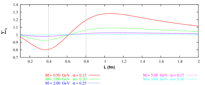
Figure 1: The figure shows the excited states finite size effect as predicted by a simplified qualitative model discussed in the text. The effective mass step scaling functions are plotted, at different values of the meson masses, as functions of the volume.

The finite volume effects due to the excited states can be easily understood by means of a two mass model for the correlation

$$f_{X}(x_{0},L)=A(L)\ e^{-M(L)x_{0}}+B(L)\ e^{-\left[M(L)+\delta M(L)\right]x_{0}}$$ (17)

Here $A(L)$ and $B(L)$ are coefficients, $M(L)$ is the meson mass and $\delta M(L)$ is the mass shift. All these quantities depend upon the physical extension of the volume $L$ but, in order to isolate the effects due to the excited states, we consider $M$ and $\delta M$ constants. In this simplified model the effective mass of eq. (16) takes the form

$$aM_{X}(x_{0})=aM+\frac{1}{2}\ln\left\{\frac{1+\frac{B(L)}{A(L)}\ e^{-\delta M(x_{0}-a)}\ }{1+\frac{B(L)}{A(L)}\ e^{-\delta M(x_{0}+a)}}\right\}$$ (18)

As in numerical simulations, we take $x_{0}=L$. The functional dependence upon the volume of the ratio $B(L)/A(L)$ can be inferred from the data on the meson decay constants given in [8, 9]. A parametrization that fits well the data is given by

$$A(L)=\alpha\left(1+\frac{0.6}{L^{2}}\right)\qquad B(L)=-0.5$$ (19)

In Fig. [1] are shown the plots of the effective mass step scaling function, as derived from this model, defined by

$$\Sigma_{X}(L)=\frac{M_{X}(2L)}{M_{X}(L)}$$ (20)

as functions of the volume and at different values of the meson masses. At the volume $L=0.4$ fm the step scaling functions are smaller than one while, the pattern is reversed at $L=0.8$ fm. Independently from the volume, the heavier mesons are closer to unity than the lighter ones.
The qualitative predictions of this simple model well reproduces the behavior of the numerically measured step scaling functions, shown in Fig. [3] for $L=0.4$ fm and in Fig. [6] for $L=0.8$ fm.

4 Step scaling functions and HQET

In this section we enter into the details of the application of the SSM, illustrated in sec. 2, to the particular case of the heavy–light meson masses computation. We introduce the step scaling functions

$$\sigma_{P}\left(L,m^{RGI}_{1},m^{RGI}_{2}\right)=\frac{\left.M_{P}\left(m^{RGI}_{1},m^{RGI}_{2}\right)\right|_{2L}}{\left.M_{P}\left(m^{RGI}_{1},m^{RGI}_{2}\right)\right|_{L}}$$

$$\sigma_{V}\left(L,m^{RGI}_{1},m^{RGI}_{2}\right)=\frac{\left.M_{V}\left(m^{RGI}_{1},m^{RGI}_{2}\right)\right|_{2L}}{\left.M_{V}\left(m^{RGI}_{1},m^{RGI}_{2}\right)\right|_{L}}$$ (21)

for the pseudoscalar and vector meson masses respectively.
To validate the expansion of eq. (3), we can make use of the HQET predictions on the heavy–light meson masses. In the infinite volume the pseudoscalar and vector meson masses have the following expansion in terms of the heavy–quark mass:

$$M_{X}(m_{h},m_{l})=m_{h}+\bar{\Lambda}(m_{l})+\frac{\alpha_{X}(m_{l})}{m_{h}}+\dots$$ (22)

where $X\in\{P,V\}$. Assuming the contribution of the $1/m^{2}_{h}$ corrections to be negligible, at finite volume one has

$$M_{X}(m_{h},m_{l},L)=m_{h}+\bar{\Lambda}_{X}(m_{l},L)+\frac{\alpha_{X}(m_{l},L)}{m_{h}}+\dots$$ (23)

where $\bar{\Lambda}_{X}(m_{l},L)$ depends upon the spin of the meson state because of the contamination of the excited states to the finite volume correlations. Using eqs. (21) and (23) we obtain the HQET predictions for the step scaling functions of the heavy-light meson masses

$$\Sigma_{X}(L,m_{h},m_{l})=1+\frac{\Sigma^{(0)}_{X}(m_{l},L)}{m_{h}}+\frac{\Sigma^{(1)}_{X}(m_{l},L)}{m_{h}^{2}}+\dots$$ (24)

This result requires some considerations. First we want to stress that in the infinite heavy–quark mass limit the step scaling functions have to be exactly equal to one, $\Sigma_{X}(L,m_{l},m_{h}\rightarrow\infty)=1$. This represents a strong constraint for the fits of the heavy–quark mass dependence of the step scaling functions.

The second observation concerns the number of terms to be considered in eq. (24). At order $O(1/m_{h})$ one has

$$\Sigma^{(0)}_{X}(m_{l},L)=\bar{\Lambda}_{X}(m_{l},2L)-\bar{\Lambda}_{X}(m_{l},L)$$ (25)

corresponding to the static approximation in eq. (23). By increasing the physical volume $L$, the difference between $\bar{\Lambda}_{X}(m_{l},2L)$ and $\bar{\Lambda}_{X}(m_{l},L)$ decreases because the two quantity have to be equal in the infinite volume limit, making the heavy–quark mass expansion of the finite volume effects rapidly convergent.
The same arguments apply to the coefficient $\Sigma^{(1)}_{X}(m_{l},L)$ that has to be considered when in the expansion of the meson masses, eq. (23), the order $O(1/m_{h})$ is taken into account.
In our calculation we will perform the fits of the step scaling functions considering the $O(1/m_{h}^{2})$ term, $\Sigma^{(1)}_{X}$, beyond the so called static evolution (SE) that retains $\Sigma^{(0)}_{X}$ only. We will also report for comparison the fits for the SE that are anyway compatible.

Similar arguments could be repeated for the heavy–heavy step scaling functions using NRQCD. In this case one cannot predict the value of the step scaling functions at $m_{h}\rightarrow\infty$. With the three simulated values of the heavy quark masses we extrapolate our numerical data with a simplified NLO formula, i.e. a linear dependence upon the heavy–quark mass, given the little sensitivity to possible slowly varying logarithmic terms.

5 Numerical results

This section contains the simulation parameters and the numerical results for each step of the calculation.

$\beta$	$L/a$	$k_{c}$	$k$	$m^{RGI}$ (GeV)
			0.120081	7.14(8)
			0.120988	6.63(7)
			0.126050	4.024(44)
6.963	$16$	0.134827(6)	0.131082	1.696(19)
			0.131314	1.591(18)
			0.134526	0.1381(30)
			0.134614	0.0978(28)
			0.134702	0.0574(28)
			0.124176	7.11(8)
			0.124844	6.61(20)
			0.128440	4.018(44)
7.300	$24$	0.134235(3)	0.131800	1.695(19)
			0.131950	1.592(18)
			0.134041	0.1374(27)
			0.134098	0.0971(24)
			0.134155	0.0567(24)
			0.126352	7.10(8)
			0.126866	6.60(7)
			0.129585	4.016(44)
7.548	$32$	0.133838(2)	0.132053	1.698(19)
			0.132162	1.595(18)
			0.133690	0.1422(27)
			0.133732	0.1021(25)
			0.133773	0.0618(23)

Table 1: Simulation parameters at $L_{0}=0.4$ fm. The RGI quark masses are obtained using eq. (12).

5.1 The small volume: $L_{0}=0.4$ fm

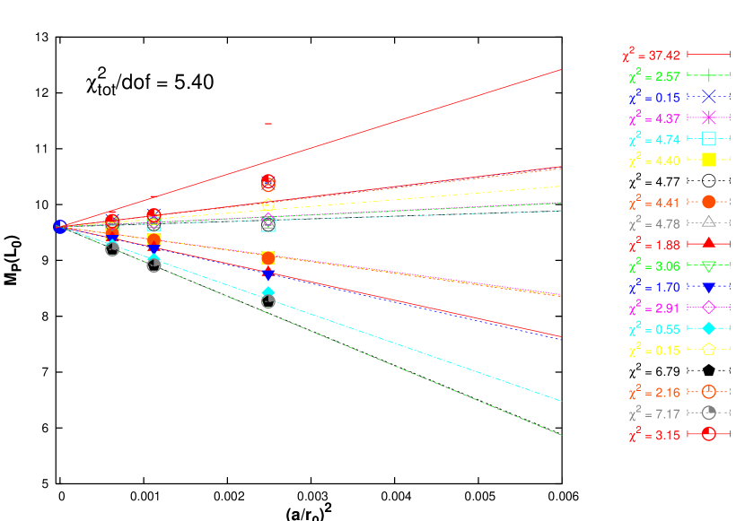
Figure 2: Continuum extrapolation on the small volume, $L_{0}$, of the mass $M_{P}(L_{0})$ of the pseudoscalar heavy–heavy meson corresponding to the heavy quark of mass $m^{RGI}=7.10$ GeV. The different values of the meson mass correspond to different definitions of the RGI quark masses given in equations (12), (13) and (14). Units are in GeV. Similar plots can be obtained, from the data reported in Table [6,7,8], for the other combinations of quark masses used in our simulations, also in the case of $M_{V}(L_{0})$.

The physical extension of the small volume has been chosen in order to properly account the dynamics of quarks with masses in the region of the the physical $b$–quark; we have fixed it to be $L_{0}=0.4$ fm. In order to have a continuum extrapolation of the numerical results, this volume has been simulated using three different discretization, $32\times 16^{3}$, $48\times 24^{3}$ and $64\times 32^{3}$. Using the results reported in [25] we have fixed two heavy quark masses with values interpolating the $b$–quark mass. In the renormalization group invariant (RGI) scheme fixed by the conventions reported in [22, 16], these masses are $7.10$ GeV and $6.60$ GeV respectively. Two other heavy quarks have been simulated in order to interpolate the mass region where, using the results reported in [26, 25], one expects to find the physical $c$–quark, i.e. $1.70$ GeV and $1.60$ GeV respectively. The charm quark mass is affordable also by a direct computation: here the calculation via our step scaling method represents a check of the procedure. An additional heavy quark has been simulated with mass $4.00$ GeV. Three light quark have been simulated with masses of $0.14$ GeV, $0.10$ GeV and $0.06$ GeV. Using the accurate determination of the RGI strange quark mass given in [27] we have fixed one of the simulated light quarks to be the physical $s$. All the parameters of the three different simulations are summarized in Table [1]. The numerical results of the pseudoscalar and vector meson masses, $M_{P}$ and $M_{V}$, are shown in Table [6,7,8] both for the heavy–heavy and for the heavy–light quark anti–quark pairs.

$\beta$	$L_{0}/a$	$k_{c}$	$k$	$m^{RGI}$ (GeV)
			0.120674	3.543(39)
			0.122220	3.114(34)
			0.126937	1.927(21)
6.420	$8$	0.135703(9)	0.134304	0.3007(36)
			0.134770	0.2003(28)
			0.135221	0.1028(21)
			0.1249	3.542(39)
			0.1260	3.136(34)
			0.1293	1.979(22)
6.737	$12$	0.135235(5)	0.1343	0.3127(38)
			0.1346	0.2090(28)
			0.1349	0.1080(21)
			0.127074	3.549(39)
			0.127913	3.153(35)
			0.130409	2.003(22)
6.963	$16$	0.134832(4)	0.134145	0.3134(38)
			0.134369	0.2112(28)
			0.134593	0.1086(20)

Table 2: Simulation parameters for the first evolution step $L_{0}\to L_{1}=0.8$ fm. The RGI quark masses are obtained using eq. (12).

In order to obtain physical predictions from the simulated data on this finite volume we need to extrapolate our numerical results to the continuum. As already mentioned, we have obtained different set of data by using the different definitions of the RGI quark masses given in the equations (12), (13) and (14). The continuum results are thus obtained trough a combined fit of all the set of data, linear in $(a/r_{0})^{2}$, as shown in Fig. [2] in the case of the mass of the pseudoscalar heavy–heavy meson corresponding to the heavy quark of mass $m^{RGI}=7.10$ GeV. We obtain a global $\chi^{2}/dof=5.40$ to be compared with the $\chi^{2}$s of each individual definition listed in the figure. We also show the points at the largest lattice spacing not included in the fit.
The errors included in the evaluation of the $\chi^{2}$ are statistical only. These are calculated by a jackknife procedure, also in the case of the step scaling functions. The systematics due to the uncertainty on the lattice spacing has been estimated by repeating the fit using the different values of the scale allowed by the uncertainties quoted in [10, 11, 12] and considering the spread of the results. The same procedure has been used for the systematics due to the uncertainties on the renormalization constants. The resulting $2\%$ percent for the renormalization constants and $1\%$ percent for the scale are summed in quadrature and added to the statistical errors.

5.2 The first evolution step: $L_{0}\mapsto L_{1}=0.8$ fm

The finite volume effects on the quantities calculated at $L_{0}$, are measured doubling the volume, $L_{1}=0.8$ fm, by using the step scaling functions of eqs. (21).
In order to have results in the continuum, also in the case of the step scaling functions three different discretizations of $L_{0}$ have been used, i.e $16\times 8^{3}$, $24\times 12^{3}$ and $32\times 16^{3}$. The volume $L_{1}$ has been simulated starting from the discretizations of $L_{0}$, fixing the value of the bare coupling and doubling the number of lattice points in each direction.

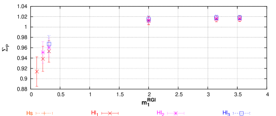
Figure 3: The figure shows the pseudoscalar step scaling functions $\Sigma_{P}$ as functions of $m_{1}^{RGI}$, for the simulation of the first evolution step corresponding to $\beta=6.963$. The different sets of data correspond to the values of $m_{2}^{RGI}$. As can be seen the step scaling functions approach a plateau for high values of $m_{1}^{RGI}$. Similar plots can be obtained using the data of Table [9,10,11] for the other values of the bare coupling and for the vector mesons step scaling functions $\Sigma_{V}$.

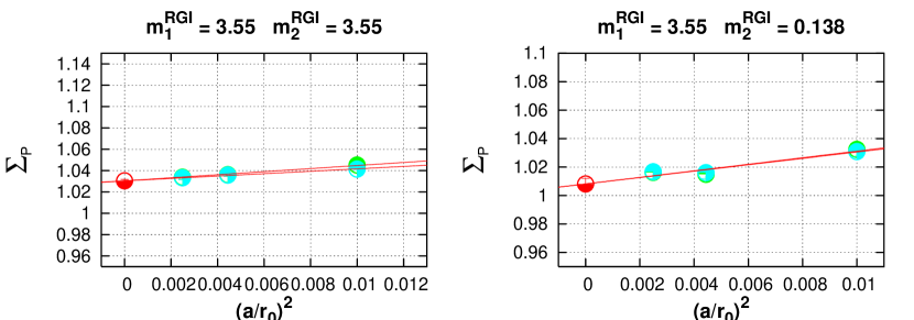
Figure 4: Continuum extrapolation on the first evolution step, $L_{0}\mapsto L_{1}$, of the step scaling function, $\Sigma_{P}(L_{0})$, of the pseudoscalar meson corresponding to the heavy quark of mass $m_{1}^{RGI}=3.55$ GeV. The two sets of data are obtained using the two definitions of RGI quark masses of equations (12) and (14). Units are in GeV. Similar plots can be obtained, from the data reported in Table [9,10,11], for the other combinations of quark masses used in our simulations, also in the case of $\Sigma_{V}(L_{0})$.

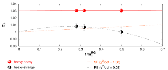
Figure 5: The figure shows the continuum extrapolated step scaling functions $\sigma_{P}(L_{0})$ as functions of $1/m_{1}^{RGI}$. The heavy extrapolations are shown only for the heavy–strange (Hs) set of data. Similar plots can be obtained using the data of Table [9,10,11] for the vector mesons step scaling functions $\sigma_{V}(L_{0})$.

The simulated quark masses have been halved with respect to the masses simulated on the small volume in order to have the same order of discretization effects proportional to $am$. The set of parameters for the simulations of this evolution step is reported in Table [2] and the numerical results are given in Table [9,10,11].

The step scaling functions of the pseudoscalar mesons at $\beta=6.963$ are plotted, at fixed $m^{RGI}_{2}$, as functions of $m^{RGI}_{1}$ in Fig. [3]. The value of the step scaling functions for the $s$ quark are obtained trough linear interpolation.

Both $\Sigma_{P}$ and $\Sigma_{V}$ are almost flat in a region of heavy quark masses starting around the charm mass. The hypothesis of low sensitivity upon the high–energy scale is thus verified.
In Fig. [4] are reported the results of the continuum extrapolation of the step scaling function, $\Sigma_{P}(L_{0})$, of the pseudoscalar meson corresponding the heavy quark of mass $m_{1}^{RGI}=3.55$ GeV.
The residual heavy mass dependence of the continuum extrapolated step scaling functions is very mild, as shown in Fig. [5] in the plot of $\sigma_{P}$ as a function of the inverse quark mass.
In the heavy–light case, as already discussed in sec. 4, we extract the values of the step scaling functions at the values of the heavy–quark masses simulated on the small volume by interpolation between the numerical results and the theoretical point at $m_{h}^{RGI}\rightarrow\infty$ using both a linear fit (SE) and a quadratic fit (RE). In the heavy–heavy case the results are linearly extrapolated.

$\beta$	$L_{1}/a$	$k_{c}$	$k$	$m^{RGI}$ (GeV)
			0.118128	2.012(22)
			0.121012	1.551(17)
			0.122513	1.337(15)
5.960	$8$	0.13490(4)	0.131457	0.3154(36)
			0.132335	0.2322(28)
			0.133226	0.1466(44)
			0.124090	1.984(22)
			0.126198	1.584(17)
			0.127280	1.389(15)
6.211	$12$	0.135831(8)	0.133574	0.3493(39)
			0.134177	0.2550(29)
			0.134786	0.1510(19)
			0.126996	1.933(21)
			0.128646	1.547(17)
			0.129487	1.355(14)
6.420	$16$	0.135734(5)	0.134318	0.3016(34)
			0.134775	0.2038(24)
			0.135235	0.1055(15)

Table 3: Simulation parameters for the first evolution step $L_{1}\to L_{2}=1.6$ fm. The RGI quark masses are obtained using eq. (12).

5.3 The second evolution step: $L_{1}\mapsto L_{2}=1.6$ fm

Figure 6: The figure shows the pseudoscalar step scaling functions $\Sigma_{P}$ as functions of $m_{1}^{RGI}$, for the simulation of the second evolution step corresponding to $\beta=6.420$. The different sets of data correspond to the values of $m_{2}^{RGI}$. Similar graphs can be obtained using the data of Table [12,13,14] for the other values of the bare coupling and for the vector mesons step scaling functions $\Sigma_{V}$.

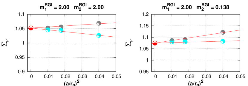
Figure 7: Continuum extrapolation on the second evolution step, $L_{1}\mapsto L_{2}$, of the step scaling function, $\Sigma_{P}(L_{1})$, of the pseudoscalar meson corresponding to the heavy quark of mass $m_{1}^{RGI}=2.00$ GeV. The two sets of data are obtained using the two definitions of RGI quark masses of equations (12) and (14). Units are in GeV. Similar plots can be obtained, from the data reported in Table [12,13,14], for the other combinations of quark masses used in our simulations, also in the case of $\Sigma_{V}(L_{1})$.

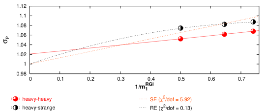
Figure 8: The figure shows the continuum extrapolated step scaling functions $\sigma_{P}(L_{1})$ as functions of $1/m_{1}^{RGI}$. The heavy extrapolations are shown only for the heavy–strange (Hs) set of data. Similar plots can be obtained using the data of Table [12,13,14] for the vector mesons step scaling functions $\sigma_{V}(L_{1})$.

In order to have the results on a physical volume, $L_{2}=1.6$ fm, a second evolution step it is required. This is done computing the meson mass step scaling functions of eq. (21) at $L=L_{1}$, by the procedure outlined in the previous section. The parameters of the simulations are given in Table [3] and the results are in Table [12,13,14].

Also in this case, the values of the simulated quark masses have been halved with respect to the previous step, owing to the lower values of the simulation cutoffs. In Fig. [6] we show the pseudoscalar step scaling functions at $\beta=6.420$ and in Fig. [8] the residual heavy–quark mass dependence with the SE and RE fits.

Fig. [7] shows the continuum extrapolation of the step scaling function, $\Sigma_{P}(L_{1})$, of the pseudoscalar meson corresponding to the heavy quark of mass $m_{1}^{RGI}=2.00$ GeV.

The contributions of the excited states, predicted from the simple model of eq. (20) and present in our numerical data, should disappear in a third evolution step. A check supporting this hypothesis is that on the larger volumes used in the simulation of this evolution step, i.e. $L_{2}$ at $\beta=6.420$ and $\beta=6.211$, the values of the meson masses defined at $x_{0}=T/2$ coincide, within the errors, with the values coming from a single mass fit to the correlations.

6 Physical results

$\qquad m_{h}^{RGI}\qquad$	State	$\qquad M_{P}\qquad$	$\qquad M_{V}\qquad$
	$\bar{h}h$	10.11(22)	10.12(22)
7.10	$\bar{h}s$	5.48(13)	5.52(13)
	$\bar{h}u$	5.40(16)	5.44(16)
	$\bar{h}h$	9.49(21)	9.50(21)
6.60	$\bar{h}s$	5.18(12)	5.22(12)
	$\bar{h}u$	5.10(15)	5.14(15)
	$\bar{h}h$	6.18(14)	6.20(14)
4.00	$\bar{h}s$	3.55(8)	3.62(8)
	$\bar{h}u$	3.46(10)	3.53(11)
	$\bar{h}h$	3.15(7)	3.21(7)
1.70	$\bar{h}s$	1.97(5)	2.09(5)
	$\bar{h}u$	1.88(6)	2.00(6)
	$\bar{h}h$	3.01(7)	3.07(7)
1.60	$\bar{h}s$	1.90(5)	2.01(5)
	$\bar{h}u$	1.80(5)	1.93(6)

Table 4: Meson masses in the infinite volume limit. Units are in GeV.

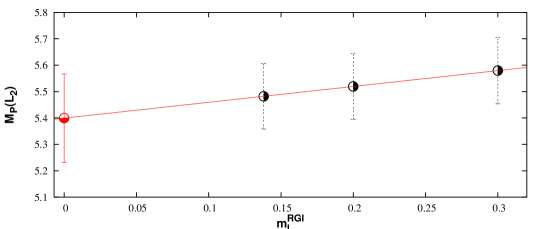
Figure 9: Chiral extrapolation of the continuum results for the pseudoscalar meson corresponding to $m_{h}^{RGI}=7.1$. Units are in GeV.

In this section we combine the results of the small volume with the results of the step scaling functions to obtain, according to eq. (4), the physical numbers. In Table [4] we give the pseudoscalar and vector meson masses corresponding to the heavy quarks simulated on the small volume and, in the heavy–light case, to strange and up light quarks. The results corresponding to the up quark have been obtained by extrapolating the continuum data in the large volume from masses around the strange region. In Figure [9] we show the extrapolation for the pseudoscalar meson corresponding to $m_{h}^{RGI}=7.1$ GeV. Having simulated three light quark on the largest volume we have fitted the results linearly without trying complicated functional forms requiring more than two parameters. Comparing these results with the experimental determinations of the same quantities [25] we obtain different determinations of the $b$–quark mass, depending upon the physical state used as experimental input. The results are summarized in Table [5].

State	$m^{RGI}_{h}$
	from P	from V
$\bar{b}b$	6.44(14)	6.57(14)
$\bar{b}s$	6.91(16)	6.93(16)
$\bar{b}u$	6.90(20)	6.91(20)
$\bar{c}c$	1.603(35)	1.642(36)
$\bar{c}s$	1.692(38)	1.741(39)
$\bar{c}u$	1.690(50)	1.712(51)

Table 5: Determinations of the heavy quark masses from the heavy–heavy and from the heavy–light states. The errors include our estimate of the systematics. Units are in GeV.

Within the quenched approximation, the determinations of the quark masses coming from the heavy–heavy or from the heavy–light spectrum in principle differ because the theory does not account for the fermion loops. We obtain two determinations that are marginally compatible within the errors and that might suggest the need for a tiny unquenching effect. The good agreement between the determinations of the quark masses coming from the heavy–up and heavy–strange sets of data make us confident on our chiral extrapolations. Of course the heavy–strange and the heavy–heavy case are not extrapolated at all and we therefore use these results only to determine the heavy–quark masses. The numbers we quote as final results are obtained by averaging the four results in the first two rows of the two sets of Table [5] for the heavy-heavy and the heavy-strange cases and by keeping the typical error of a single case:

$$m_{b}^{RGI}=6.73(16)\mbox{ GeV}\qquad\qquad m_{b}^{\overline{MS}}(m_{b}^{\overline{MS}})=4.33(10)\mbox{ GeV}$$ (26)

for the $b$–quark and

$$m_{c}^{RGI}=1.681(36)\mbox{ GeV}\qquad\qquad m_{c}^{\overline{MS}}(m_{c}^{\overline{MS}})=1.319(28)\mbox{ GeV}$$ (27)

for the charm. The latter results compare favorably with the results of the direct computations [26, 25].

As already explained in section 5.1, our error estimate includes both the statistical error from the Monte Carlo simulation as well as the systematic error coming from the uncertainty on the lattice spacing corresponding at a given $\beta$ value and to the uncertainty on the renormalization constants in eqs (10) and (14). The final errors on the continuum quantities, of the order of $2\%$ percent for the renormalization constants and of about $1\%$ percent for the scale, are summed in quadrature and added to the statistical errors. The evolution to the $\overline{MS}$ scheme has been done using four–loop renormalization group equations [28, 29, 30].

Using these determinations of the quark masses we can calculate the mass of the $B_{c}$ meson from our set of correlations suitably interpolated. Following this procedure we obtain a determination that is in very good agreement with the experimental measurement of the meson mass [25]:

$$M_{B_{c}}=6.46(15)\mbox{ GeV}\qquad M_{B_{c}}^{exp}=6.40(39)(13)\mbox{ GeV}$$ (28)

The same analysis has been done also in the case of the decay constants and in [9] we give the first determination of $f_{B_{c}}$ from lattice QCD in the quenched approximation.

7 Conclusions

We have shown the effectiveness of the step scaling method in the computation of the heavy–light and heavy–heavy meson spectrum. We have performed the calculations for the pseudoscalar and vector mesons in the continuum limit of lattice QCD in the quenched approximation and, by comparison with the experimental determinations, we have extracted the masses of the bottom and of the charm quarks.
Our results represent the first determination of the bottom quark mass in the continuum limit of quenched lattice QCD.

Using the results on the quark masses we give an independent theoretical calculation of the $B_{c}$ meson mass that matches very well the experimental result.

$\qquad\qquad\beta\qquad\qquad$	$\qquad m_{1}^{RGI}\qquad$	$\qquad m_{2}^{RGI}\qquad$	$\qquad M_{P}$	$\qquad{M}_{V}$
	7.14(8)	7.14(8)	8.295(5)	8.318(5)
		6.63(7)	8.092(5)	8.116(6)
		4.024(44)	6.898(6)	6.924(6)
		1.696(19)	5.590(7)	5.622(7)
		1.591(18)	5.527(7)	5.559(8)
		0.1381(30)	4.646(9)	4.691(10)
		0.0978(28)	4.622(10)	4.668(10)
		0.0574(28)	4.597(10)	4.645(10)
	6.63(7)	6.63(7)	7.888(5)	7.913(6)
		4.024(44)	6.693(6)	6.721(6)
		1.696(19)	5.384(7)	5.417(7)
		1.591(18)	5.320(7)	5.354(8)
		0.1381(30)	4.438(9)	4.485(10)
		0.0978(28)	4.414(10)	4.462(10)
		0.0574(28)	4.390(10)	4.440(10)
6.963	4.024(44)	4.024(44)	5.491(6)	5.524(7)
		1.696(19)	4.170(7)	4.215(8)
		1.591(18)	4.106(7)	4.152(8)
		0.1381(30)	3.207(10)	3.278(11)
		0.0978(28)	3.183(10)	3.255(11)
		0.0574(28)	3.158(10)	3.232(11)
	1.696(19)	1.696(19)	2.826(8)	2.898(9)
		1.591(18)	2.760(8)	2.835(9)
		0.1381(30)	1.816(10)	1.952(12)
		0.0978(28)	1.790(10)	1.928(12)
		0.0574(28)	1.763(10)	1.905(12)
	1.591(18)	1.591(18)	2.694(8)	2.771(9)
		0.1381(30)	1.746(10)	1.888(12)
		0.0978(28)	1.719(10)	1.864(12)
		0.0574(28)	1.692(10)	1.840(12)

Table 6: Values of the pseudoscalar, $M_{P}$, and vector, $M_{V}$, meson masses resulting from the simulations on the smallest volume $L_{0}=0.4$ fm at $\beta=6.963$. Units are in GeV.

$\qquad\qquad\beta\qquad\qquad$	$\qquad m_{1}^{RGI}\qquad$	$\qquad m_{2}^{RGI}\qquad$	$\qquad M_{P}$	$\qquad{M}_{V}$
	7.11(8)	7.11(8)	8.920(6)	8.944(7)
		6.61(20)	8.678(6)	8.702(7)
		4.018(44)	7.310(7)	7.336(8)
		1.695(19)	5.926(9)	5.957(10)
		1.592(18)	5.862(9)	5.893(10)
		0.1374(27)	4.987(13)	5.031(14)
		0.0971(24)	4.964(14)	5.009(14)
		0.0567(24)	4.942(14)	4.987(15)
	6.61(20)	6.61(20)	8.435(6)	8.459(7)
		4.018(44)	7.066(7)	7.093(8)
		1.695(19)	5.680(9)	5.713(10)
		1.592(18)	5.616(9)	5.649(10)
		0.1374(27)	4.739(13)	4.786(14)
		0.0971(24)	4.717(14)	4.764(15)
		0.0567(24)	4.694(14)	4.742(15)
7.300	4.018(44)	4.018(44)	5.689(8)	5.722(9)
		1.695(19)	4.291(10)	4.336(11)
		1.592(18)	4.226(10)	4.272(11)
		0.1374(27)	3.334(14)	3.404(15)
		0.0971(24)	3.310(14)	3.381(15)
		0.0567(24)	3.287(14)	3.359(16)
	1.695(19)	1.695(19)	2.869(11)	2.942(13)
		1.592(18)	2.803(11)	2.878(13)
		0.1374(27)	1.864(14)	1.999(17)
		0.0971(24)	1.838(14)	1.976(17)
		0.0567(24)	1.812(15)	1.953(17)
	1.592(18)	1.592(18)	2.736(11)	2.813(13)
		0.1374(27)	1.793(14)	1.934(17)
		0.0971(24)	1.767(14)	1.911(17)
		0.0567(24)	1.741(15)	1.888(18)

Table 7: Values of the pseudoscalar, $M_{P}$, and vector, $M_{V}$, meson masses resulting from the simulations on the smallest volume $L_{0}=0.4$ fm at $\beta=7.300$. Units are in GeV.

$\qquad\qquad\beta\qquad\qquad$	$\qquad m_{1}^{RGI}\qquad$	$\qquad m_{2}^{RGI}\qquad$	$\qquad M_{P}$	$\qquad{M}_{V}$
	7.10(8)	7.10(8)	9.203(7)	9.225(8)
		6.60(7)	8.939(7)	8.960(8)
		4.016(44)	7.480(8)	7.503(9)
		1.698(19)	6.060(10)	6.088(10)
		1.595(18)	5.996(10)	6.025(11)
		0.1422(27)	5.115(14)	5.157(15)
		0.1021(25)	5.093(14)	5.135(15)
		0.0618(23)	5.070(15)	5.113(15)
	6.60(7)	6.60(7)	8.674(7)	8.696(8)
		4.016(44)	7.214(8)	7.238(9)
		1.698(19)	5.792(10)	5.822(11)
		1.595(18)	5.728(10)	5.759(12)
		0.1422(27)	4.846(14)	4.891(15)
		0.1021(25)	4.823(14)	4.869(15)
		0.0618(23)	4.801(15)	4.847(15)
7.548	4.016(44)	4.016(44)	5.746(9)	5.776(10)
		1.698(19)	4.314(10)	4.356(11)
		1.595(18)	4.249(10)	4.292(12)
		0.1422(27)	3.352(15)	3.420(15)
		0.1021(25)	3.328(15)	3.398(16)
		0.0618(23)	3.305(15)	3.377(16)
	1.698(19)	1.698(19)	2.860(11)	2.930(13)
		1.595(18)	2.794(11)	2.866(13)
		0.1422(27)	1.852(15)	1.988(17)
		0.1021(25)	1.827(15)	1.966(17)
		0.0618(23)	1.801(16)	1.944(18)
	1.595(18)	1.595(18)	2.727(12)	2.802(13)
		0.1422(27)	1.781(15)	1.924(17)
		0.1021(25)	1.756(15)	1.901(18)
		0.0618(23)	1.730(16)	1.879(18)

Table 8: Values of the pseudoscalar, $M_{P}$, and vector, $M_{V}$, meson masses resulting from the simulations on the smallest volume $L_{0}=0.4$ fm at $\beta=7.548$. Units are in GeV.

$\qquad\qquad\beta\qquad\qquad$	$\qquad m_{1}^{RGI}\qquad$	$\qquad m_{2}^{RGI}\qquad$	$\qquad\Sigma_{P}$	$\qquad\Sigma_{V}$
	0.1028(21)	0.1028(21)	0.996(28)	0.826(21)
		0.2003(28)	1.010(23)	0.848(19)
		0.3007(36)	1.017(20)	0.869(17)
		1.927(21)	1.034(7)	0.998(8)
		3.114(34)	1.032(5)	1.013(6)
		3.543(39)	1.031(5)	1.015(5)
	0.2003(28)	0.2003(28)	1.016(20)	0.867(17)
		0.3007(36)	1.020(18)	0.885(15)
		1.927(21)	1.036(7)	1.003(7)
		3.114(34)	1.034(5)	1.015(5)
		3.543(39)	1.037(5)	1.018(5)
6.420	0.3007(36)	0.3007(36)	1.022(16)	0.901(14)
		1.927(21)	1.038(6)	1.007(7)
		3.114(34)	1.036(5)	1.019(5)
		3.543(39)	1.0349(46)	1.0205(47)
	1.927(21)	1.927(21)	1.0520(34)	1.0425(37)
		3.114(34)	1.0493(27)	1.0438(29)
		3.543(39)	1.0479(25)	1.0433(27)
	3.114(34)	3.114(34)	1.0471(21)	1.0440(23)
		3.543(39)	1.0460(20)	1.0433(22)
	3.543(39)	3.543(39)	1.0449(19)	1.0427(20)

Table 9: Values of the step scaling functions for the pseudoscalar, $\Sigma_{P}$, and vector, $\Sigma_{V}$, meson masses resulting from the simulation at $\beta=6.420$ of the first evolution step $L_{0}\to L_{1}$. Units are in GeV.

$\qquad\qquad\beta\qquad\qquad$	$\qquad m_{1}^{RGI}\qquad$	$\qquad m_{2}^{RGI}\qquad$	$\qquad\Sigma_{P}$	$\qquad\Sigma_{V}$
	0.1080(21)	0.1080(21)	0.907(25)	0.789(19)
		0.2090(28)	0.935(21)	0.810(17)
		0.3127(38)	0.951(19)	0.830(16)
		1.979(22)	1.009(7)	0.976(7)
		3.136(34)	1.014(5)	0.995(5)
		3.542(39)	1.014(5)	0.998(5)
	0.2090(28)	0.2090(28)	0.950(18)	0.828(16)
		0.3127(38)	0.960(16)	0.846(14)
		1.979(22)	1.011(6)	0.980(7)
		3.136(34)	1.0155(47)	0.998(5)
		3.542(39)	1.0158(43)	1.0009(46)
6.737	0.3127(38)	0.3127(38)	0.967(14)	0.862(13)
		1.979(22)	1.014(6)	0.985(6)
		3.136(34)	1.0176(44)	1.0013(47)
		3.542(39)	1.0178(40)	1.0039(43)
	1.979(22)	1.979(22)	1.0376(30)	1.0279(33)
		3.136(34)	1.0375(23)	1.0317(25)
		3.542(39)	1.0367(21)	1.0317(23)
	3.136(34)	3.136(34)	1.0372(18)	1.0338(19)
		3.542(39)	1.0365(16)	1.0336(18)
	3.542(39)	3.542(39)	1.0358(15)	1.0333(17)

Table 10: Values of the step scaling functions for the pseudoscalar, $\Sigma_{P}$, and vector, $\Sigma_{V}$, meson masses resulting from the simulation at $\beta=6.737$ of the first evolution step $L_{0}\to L_{1}$. Units are in GeV.

$\qquad\qquad\beta\qquad\qquad$	$\qquad m_{1}^{RGI}\qquad$	$\qquad m_{2}^{RGI}\qquad$	$\qquad\Sigma_{P}$	$\qquad\Sigma_{V}$
	0.1086(20)	0.1086(20)	0.914(28)	0.783(24)
		0.2112(28)	0.939(24)	0.807(21)
		0.3134(38)	0.953(21)	0.830(19)
		2.003(22)	1.012(8)	0.981(8)
		3.153(35)	1.016(6)	0.999(6)
		3.549(39)	1.016(5)	1.002(6)
	0.2112(28)	0.2112(28)	0.951(21)	0.828(19)
		0.3134(38)	0.960(18)	0.847(17)
		2.003(22)	1.013(7)	0.984(8)
		3.153(35)	1.017(5)	1.001(6)
		3.549(39)	1.017(5)	1.003(5)
6.963	0.3134(38)	0.3134(38)	0.967(16)	0.864(16)
		2.003(22)	1.015(7)	0.989(7)
		3.153(35)	1.018(5)	1.004(5)
		3.549(39)	1.0181(46)	1.006(5)
	2.003(22)	2.003(22)	1.0365(35)	1.0281(39)
		3.153(35)	1.0357(27)	1.0309(30)
		3.549(39)	1.0348(25)	1.0307(28)
	3.153(35)	3.153(35)	1.0349(21)	1.0321(23)
		3.549(39)	1.0341(20)	1.0317(22)
	3.549(39)	3.549(39)	1.0333(19)	1.0313(20)

Table 11: Values of the step scaling functions for the pseudoscalar, $\Sigma_{P}$, and vector, $\Sigma_{V}$, meson masses resulting from the simulation at $\beta=6.963$ of the first evolution step $L_{0}\to L_{1}$. Units are in GeV.

$\qquad\qquad\beta\qquad\qquad$	$\qquad m_{1}^{RGI}\qquad$	$\qquad m_{2}^{RGI}\qquad$	$\qquad\Sigma_{P}$	$\qquad\Sigma_{V}$
	0.1466(44)	0.1466(44)	1.269(13)	1.308(15)
		0.2322(28)	1.244(11)	1.286(12)
		0.3154(36)	1.226(9)	1.267(10)
		1.337(15)	1.1406(40)	1.1636(45)
		1.551(17)	1.1332(37)	1.1539(42)
		2.012(22)	1.1214(32)	1.1383(36)
	0.2322(28)	0.2322(28)	1.224(9)	1.266(10)
		0.3154(36)	1.209(8)	1.249(9)
		1.337(15)	1.1337(35)	1.1557(40)
		1.551(17)	1.1268(32)	1.1467(37)
		2.012(22)	1.1158(29)	1.1322(32)
5.960	0.3154(36)	0.3154(36)	1.196(7)	1.235(8)
		1.337(15)	1.1278(32)	1.1489(37)
		1.551(17)	1.1213(30)	1.1405(34)
		2.012(22)	1.1110(27)	1.1269(30)
	1.337(15)	1.337(15)	1.0894(19)	1.029(21)
		1.551(17)	1.0853(18)	1.0978(20)
		2.012(22)	1.0785(16)	1.0895(17)
	1.551(17)	1.551(17)	1.0814(17)	1.0931(18)
		2.012(22)	1.0749(15)	1.0852(16)
	2.012(22)	2.012(22)	1.0689(13)	1.0782(14)

Table 12: Values of the step scaling functions for the pseudoscalar, $\Sigma_{P}$, and vector, $\Sigma_{V}$, meson masses resulting from the simulation at $\beta=5.960$ of the second evolution step $L_{1}\to L_{2}$. Units are in GeV.

$\qquad\qquad\beta\qquad\qquad$	$\qquad m_{1}^{RGI}\qquad$	$\qquad m_{2}^{RGI}\qquad$	$\qquad\Sigma_{P}$	$\qquad\Sigma_{V}$
	0.1510(19)	0.1510(19)	1.156(14)	1.255(18)
		0.2550(29)	1.151(11)	1.235(15)
		0.3493(39)	1.146(10)	1.219(12)
		1.389(15)	1.1035(46)	1.131(6)
		1.584(17)	1.1098(42)	1.123(5)
		1.984(22)	1.0899(37)	1.1095(44)
	0.2550(29)	0.2550(29)	1.147(10)	1.218(12)
		0.3493(39)	1.142(8)	1.204(10)
		1.389(15)	1.1010(40)	1.1258(48)
		1.584(17)	1.0961(37)	1.1181(44)
		1.984(22)	1.0879(33)	1.1056(39)
6.211	0.3493(39)	0.3493(39)	1.138(7)	1.193(9)
		1.389(15)	1.0983(37)	1.1210(44)
		1.584(17)	1.0936(34)	1.1137(40)
		1.984(22)	1.0857(30)	1.1020(35)
	1.389(15)	1.389(15)	1.0727(20)	1.0842(24)
		1.584(17)	1.0695(19)	1.0799(22)
		1.984(22)	1.0640(17)	1.0728(20)
	1.584(17)	1.584(17)	1.0664(18)	1.0759(21)
		1.984(22)	1.0611(16)	1.0692(18)
	1.984(22)	1.984(22)	1.0564(14)	1.0633(16)

Table 13: Values of the step scaling functions for the pseudoscalar, $\Sigma_{P}$, and vector, $\Sigma_{V}$, meson masses resulting from the simulation at $\beta=6.211$ of the second evolution step $L_{1}\to L_{2}$. Units are in GeV.

$\qquad\qquad\beta\qquad\qquad$	$\qquad m_{1}^{RGI}\qquad$	$\qquad m_{2}^{RGI}\qquad$	$\qquad\Sigma_{P}$	$\qquad\Sigma_{V}$
	0.1055(15)	0.1055(15)	1.167(27)	1.259(35)
		0.2038(24)	1.162(22)	1.235(27)
		0.3016(34)	1.156(18)	1.218(22)
		1.355(14)	1.104(7)	1.125(9)
		1.547(17)	1.098(7)	1.117(8)
		1.933(21)	1.088(6)	1.103(7)
	0.2038(24)	0.2038(24)	1.155(18)	1.217(21)
		0.3016(34)	1.150(15)	1.203(18)
		1.355(14)	1.101(6)	1.121(8)
		1.547(17)	1.095(6)	1.113(7)
		1.933(21)	1.086(5)	1.000(6)
6.420	0.3016(34)	0.3016(34)	1.144(13)	1.192(16)
		1.355(14)	1.098(6)	1.118(7)
		1.547(17)	1.093(5)	1.110(6)
		1.933(21)	1.0839(46)	1.098(5)
	1.355(14)	1.355(14)	1.0711(31)	1.0821(37)
		1.547(17)	1.0676(29)	1.0777(34)
		1.933(21)	1.0617(25)	1.0702(30)
	1.547(17)	1.547(17)	1.0643(27)	1.0735(31)
		1.933(21)	1.0587(24)	1.0665(27)
	1.933(21)	1.933(21)	1.0538(21)	1.0604(24)

Table 14: Values of the step scaling functions for the pseudoscalar, $\Sigma_{P}$, and vector, $\Sigma_{V}$, meson masses resulting from the simulation at $\beta=6.420$ of the second evolution step $L_{1}\to L_{2}$. Units are in GeV.

References

- [1] H. Wittig, (2002), hep-lat/0210025.
- [2] V. Gimenez et al., JHEP 03 (2000) 018, hep-lat/0002007.
- [3] HPQCD, A. Gray et al., (2002), hep-lat/0209022.
- [4] C.W. Bauer et al., (2002), hep-ph/0210027.
- [5] M. Battaglia et al., (2002), hep-ph/0210319.
- [6] R. Sommer, (2002), hep-lat/0209162.
- [7] J. Heitger, M. Kurth and R. Sommer, (2003), hep-lat/0302019.
- [8] M. Guagnelli et al., Phys. Lett. B546 (2002) 237, hep-lat/0206023.
- [9] G.M. de Divitiis et al., Work in preparation.
- [10] ALPHA, M. Guagnelli, R. Sommer and H. Wittig, Nucl. Phys. B535 (1998) 389, hep-lat/9806005.
- [11] S. Necco and R. Sommer, Nucl. Phys. B622 (2002) 328, hep-lat/0108008.
- [12] M. Guagnelli, R. Petronzio and N. Tantalo, Phys. Lett. B548 (2002) 58, hep-lat/0209112.
- [13] M. Luscher et al., Nucl. Phys. B384 (1992) 168, hep-lat/9207009.
- [14] S. Sint, Nucl. Phys. B421 (1994) 135, hep-lat/9312079.
- [15] M. Luscher et al., Nucl. Phys. B413 (1994) 481, hep-lat/9309005.
- [16] S. Capitani et al., Nucl. Phys. Proc. Suppl. 63 (1998) 153, hep-lat/9709125.
- [17] ALPHA, A. Bode et al., Phys. Lett. B515 (2001) 49, hep-lat/0105003.
- [18] Zeuthen-Rome / ZeRo, M. Guagnelli et al., (2003), hep-lat/0303012.
- [19] M. Luscher et al., Nucl. Phys. B491 (1997) 323, hep-lat/9609035.
- [20] M. Guagnelli and R. Sommer, Nucl. Phys. Proc. Suppl. 63 (1998) 886, hep-lat/9709088.
- [21] S. Sint and P. Weisz, Nucl. Phys. B502 (1997) 251, hep-lat/9704001.
- [22] J. Gasser and H. Leutwyler, Nucl. Phys. B250 (1985) 465.
- [23] G.M. de Divitiis and R. Petronzio, Phys. Lett. B419 (1998) 311, hep-lat/9710071.
- [24] ALPHA, M. Guagnelli et al., Nucl. Phys. B595 (2001) 44, hep-lat/0009021.
- [25] Particle Data Group, K. Hagiwara et al., Phys. Rev. D66 (2002) 010001.
- [26] ALPHA, J. Rolf and S. Sint, JHEP 12 (2002) 007, hep-ph/0209255.
- [27] ALPHA, J. Garden et al., Nucl. Phys. B571 (2000) 237, hep-lat/9906013.
- [28] T. van Ritbergen, J.A.M. Vermaseren and S.A. Larin, Phys. Lett. B400 (1997) 379, hep-ph/9701390.
- [29] J.A.M. Vermaseren, S.A. Larin and T. van Ritbergen, Phys. Lett. B405 (1997) 327, hep-ph/9703284.
- [30] K.G. Chetyrkin, Phys. Lett. B404 (1997) 161, hep-ph/9703278.