Hybrid configuration content of heavy S-wave mesons

Abstract

We use the non-relativistic expansion of QCD (NRQCD) on the lattice to study the lowest hybrid configuration contribution to the ground state of heavy S-wave mesons. Using lowest-order lattice NRQCD to create the heavy-quark propagators, we form a basis of “unperturbed” S-wave and hybrid states. We then apply the lowest-order coupling of the quark spin and chromomagnetic field at an intermediate time slice to create “mixed” correlators between the S-wave and hybrid states. From the resulting amplitudes, we extract the off-diagonal element of our two-state Hamiltonian. Diagonalizing this Hamiltonian gives us the admixture of hybrid configuration within the meson ground state. The present effort represents a continuation of previous work: the analysis has been extended to include lattices of varying spacings, source operators having better overlap with the ground states, and the pseudoscalar (along with the vector) channel. Results are presented for bottomonium ($\Upsilon$, $\eta_{b}$) using three different sets of quenched lattices. We also show results for charmonium ($J/\psi$, $\eta_{c}$) from one lattice set, although we note that the non-relativistic approximation is not expected to be very good in this case.

I Introduction

The existence of valence gluons in bound quark systems, a theoretical possibility considered for a long time in QCD, continues to elude confirmation. Allowance for gluonic excitations increases the range of possible hadronic quantum numbers ($J^{PC}$) beyond those predicted by constituent quark models. Exotic states should appear (for recent reviews see Refs. Michael (2003); Barnes (2003a)) and, in fact, one such state ($1^{-+}$) has been observed recently Ivanov et al. (2001), but the underlying structure of the state (hybrid meson, four-quark state, meson molecule, etc.) has not been determined. When considering gluonic constituents, however, the resulting state need not be exotic; the valence gluons may also combine with the quarks and antiquarks to form a state which may otherwise be formed without the gluonic presence. In this non-exotic scenario, a meson (or baryon) state should consist of a mixture of configurations; not only the case where only the valence quarks and antiquarks appear, but also those where a gluonic excitation is present: a hybrid configuration.

As a relevant example – since this is one of the systems we study in the present work – we may look at the vector meson state for bottomonium ($\Upsilon$, $1^{--}$). We may envision the ground state for this system as a bottom quark and antiquark in a color singlet, a relative S-wave, and a spin triplet. However, the true ground state should also have a contribution where the quark and antiquark are in a spin singlet and a color octet, the spin of the meson and the overall color singlet being ensured by the gluonic excitation:

$$|\Upsilon\rangle = \hskip 7.68236pt{\cal A}_{s}|b\bar{b}\rangle\hskip 29.02193pt+\hskip 5.40608pt{\cal A}_{h}|b\bar{b}g\rangle$$ (1)

$$= \cos\theta|1S(1^{--})\rangle+\sin\theta|1H(1^{--})\rangle.$$

It is just this type of (albeit simplified) two-state system we consider in the present work. We also consider the $0^{-+}$ heavy S-wave meson:

$$|\eta_{b}\rangle=\cos\theta^{\prime}|1S(0^{-+})\rangle+\sin\theta^{\prime}|1H(0^{-+})\rangle.$$ (2)

Hybrid-quarkonium configuration mixing has been considered before in the framework of the MIT bag model Barnes (1979); de Viron (1984) and with the use of an adiabatic potential model Gerasimov (1998). We compare results from this on-going lattice work Burch et al. (2001, 2002); Burch (2003) with these previous results.

II Lattice method

We work in the heavy-quark limit, so we use the non-relativistic expansion of lattice QCD Caswell and Lepage (1986); Eichten (1987); Lepage and Thacker (1987). To evolve our quark propagators we use a time-step-symmetric form for the transfer matrix Lepage et al. (1992); Burch et al. (2001):

$$\phi(\vec{x},t+a)=\left(1-\frac{a{\cal H}_{0}}{2n}\right)_{t+a}^{n}U^{\dagger}_{4}(x)\left(1-\frac{a{\cal H}_{0}}{2n}\right)_{t}^{n}$$

$$\times(1-\delta_{t^{\prime},t}a\delta{\cal H})_{t}\,\phi(\vec{x},t).$$ (3)

The Hamiltonian applied at all time slices, ${\cal H}_{0}$, accounts for the kinetic energy of the heavy quarks:

$${\cal H}_{0}=-\frac{\Delta^{2}}{2m_{q}},$$ (4)

where the $\Delta^{2}$ is the lattice covariant Laplacian. At one intermediate time slice, $t^{\prime}$, the lowest-order spin-dependent interaction,

$$\delta{\cal H}=-c_{B}\frac{g}{2m_{q}}\vec{\sigma}\cdot\vec{B},$$ (5)

is applied, thereby allowing a spin flip of the quark (or antiquark) in exchange for the emission or absorption of a gluonic excitation; i.e., configuration mixing.

The local value of the chromomagnetic field is calculated using the clover formulation, averaging the fields generated from the four plaquettes surrounding a lattice site:

$$\Omega_{\mu\nu}(x) = \frac{1}{4}\left[U_{\mu}(x)U_{\nu}(x+\hat{\mu})U^{\dagger}_{\mu}(x+\hat{\nu})U^{\dagger}_{\nu}(x)\right.$$ (6)

$$\left.+\,U_{\nu}(x)U^{\dagger}_{\mu}(x+\hat{\nu}-\hat{\mu})U^{\dagger}_{\nu}(x-\hat{\mu})U_{\mu}(x-\hat{\mu})\right.$$

$$\left.+\,U^{\dagger}_{\mu}(x-\hat{\mu})U^{\dagger}_{\nu}(x-\hat{\nu}-\hat{\mu})U_{\mu}(x-\hat{\nu}-\hat{\mu})U_{\nu}(x-\hat{\nu})\right.$$

$$\left.+\,U^{\dagger}_{\nu}(x-\hat{\nu})U_{\mu}(x-\hat{\nu})U_{\nu}(x-\hat{\nu}+\hat{\mu})U^{\dagger}_{\mu}(x)\right],$$

$${\cal F}_{\mu\nu}(x)=\frac{1}{2i}\left[\Omega_{\mu\nu}(x)-\Omega_{\mu\nu}^{\dagger}(x)\right]-\frac{1}{3}{\rm Im}[{\rm Tr}\,\Omega_{\mu\nu}(x)].$$ (7)

The chromomagnetic field arises from the spatial components,

$${\cal F}_{jk}(x)=-\varepsilon_{jkl}gB_{l}(x).$$ (8)

Tadpole improvement Lepage and Mackenzie (1993) is also included, the factor $u_{0}$ being calculated via the average plaquette and applied to all the link variables:

$$U_{\mu}(x)\rightarrow\frac{U_{\mu}(x)}{u_{0}}\hskip 5.69046pt;\hskip 5.69046pt{\cal F}_{\mu\nu}(x)\rightarrow\frac{{\cal F}_{\mu\nu}(x)}{u_{0}^{4}}.$$ (9)

Creating the heavy-quark propagators with this form for the evolution operator, we then use appropriate operators at the source and sink time slices to project out the desired meson states. The heavy-meson operators we use, along with the corresponding quantum numbers, may be found in Table 1 of Ref. Burch et al. (2001).

Two different types of quark sources are used: a random wall (RW) and a Coulomb-gauge-fixed wall (CW). The RW source is an incoherent collection of point sources, the average meson propagator having contributions only from where the quark and antiquark start at the same location. The CW source provides a “maximally smeared” source, with contributions from spatially separated quarks and antiquarks. In both cases, the sink end is simply a sum over points where both the quark and antiquark coexist.

We fit the S-wave propagator with the following form:

$$C_{s}(t)=A_{1s}e^{-m_{1s}t}+A_{2s}e^{-m_{2s}t},$$ (10)

allowing a determination of the 2S-1S mass splitting. We also have P-wave correlators, which we fit (at least for the CW source) with only a single mass,

$$C_{p}(t)=A_{2p}e^{-m_{2p}t}.$$ (11)

We use the 2P-1S mass splitting to set the lattice scale. A single-mass fit is also used for the hybrid correlators,

$$C_{h}(t)=A_{1h}e^{-m_{1h}t}.$$ (12)

All fits to the propagators use the full covariance matrix to account for correlations among the different Euclidean times.

After application of the spin-dependent term in the Hamiltonian at $t^{\prime}$ (or $t^{\prime\prime}$), a signal appears for the “mixed” correlator, hybrid $\rightarrow$ S-wave (or vice versa). We fit these correlators in the region $t>t^{\prime}$ (or $t>t^{\prime\prime}$) with the forms:

$$C_{hs}^{(1)}(t^{\prime},t)=A_{1hs}(t^{\prime})e^{-m_{1s}(t-t^{\prime})}$$ (13)

and

$$C_{sh}^{(1)}(t^{\prime\prime},t)=A_{1sh}(t^{\prime\prime})e^{-m_{1h}(t-t^{\prime\prime})}.$$ (14)

Looking more closely at the amplitude for the first correlator (hybrid $\rightarrow$ S-wave), we can reason that there should be factors from the overlap of the source operator with the hybrid, the overlap of the sink operator with the S-wave, the exponential decay of the hybrid state before $t^{\prime}$, and the matrix element with which we are interested:

$$A_{1hs}(t^{\prime})=A_{1h}^{1/2}A_{1s}^{1/2}\left\langle 1S\left|a\delta{\cal H}\right|1H\right\rangle e^{-m_{1h}t^{\prime}}.$$ (15)

Knowing the masses and amplitudes from the standard S-wave and hybrid correlators, we solve for the off-diagonal matrix element of our two-state Hamiltonian. This is repeated for larger values of $t^{\prime}$ to find a plateau in the final result, where we may be sure that only the ground-state contribution from the source appears. A similar procedure may be followed for the S-wave $\rightarrow$ hybrid correlator.

There is a complication, however, which arises for our CW-source correlators: the operators at the source and sink ends are not the same. At one end we have a Coulomb-gauge-fixed wall ($cw$) source, while at the other end there is a point ($p$) sink. The amplitude for the S-wave correlator therefore has the form

$$A_{1s}=A_{1s_{cw}}^{1/2}A_{1s_{p}}^{1/2},$$ (16)

while that for the hybrid is

$$A_{1h}=A_{1h_{cw}}^{1/2}A_{1h_{p}}^{1/2}.$$ (17)

From each of these products, the mixed correlators include only one of the factors (rather than just the square root of each amplitude):

$$A_{1hs}(t^{\prime})=A_{1s_{p}}^{1/2}A_{1h_{cw}}^{1/2}\left\langle 1S\left|a\delta{\cal H}\right|1H\right\rangle e^{-m_{1h}t^{\prime}}$$ (18)

and

$$A_{1sh}(t^{\prime\prime})=A_{1h_{p}}^{1/2}A_{1s_{cw}}^{1/2}\left\langle 1H\left|a\delta{\cal H}\right|1S\right\rangle e^{-m_{1s}t^{\prime\prime}}.$$ (19)

In order to get the appropriate cancellations of amplitudes, we thus need to use a geometric mean:

$$\left|\left\langle 1S\left|a\delta{\cal H}\right|1H\right\rangle\right|=\sqrt{\frac{A_{1hs}(t^{\prime})A_{1sh}(t^{\prime\prime})}{A_{1s}A_{1h}}e^{m_{1h}t^{\prime}}e^{m_{1s}t^{\prime\prime}}}$$ (20)

at large $t^{\prime},t^{\prime\prime}$.

We average the correlators over sets of quenched lattices, generated using a Symanzik 1-loop improved gauge action Symanzik (1983); Luscher and Weisz (1985); Lepage and Mackenzie (1993); Alford et al. (1995); Bernard et al. (1998). The relevant parameters for these runs are listed in Table 1.

Table 1: Quenched NRQCD runs.

$\beta$	$N_{s}^{3}\times N_{t}$	$u_{0}$	$am_{q}$	$n$	sources	# configs.
7.75	$16^{3}\times 32$	0.8800	3.2, 3.6	2	RW,CW	220
8.00	$20^{3}\times 64$	0.8879	2.5, 2.8	2	RW,CW	240
′′	′′	′′	0.7, 0.8	3	CW	170
8.40	$28^{3}\times 96$	0.89741	1.8, 2.0	2	RW,CW	76

To set the physical scale for the lattice spacing and determine the physical quark mass, we use the same procedure as was used previously for bottomonium spectroscopy with NRQCD Davies et al. (1994). For the lattice spacings, we use bottomonium mass splittings, such as the spin-averaged 2P-1S mass difference ($M_{\bar{\chi}_{b}}-M_{\Upsilon}=440$ MeV) and the 2S-1S difference for the $\Upsilon$ ($M_{\Upsilon^{\prime}}-M_{\Upsilon}=563$ MeV). We also create non-zero-momentum S-wave correlators and use the resulting dispersion relations to determine the kinetic masses of the ground states. Using the results from two quark masses, an interpolation (or extrapolation) may be made to match the kinetic S-wave mass to that of the $\Upsilon$ ($M_{\Upsilon}=9.46$ GeV), thus arriving at a physical bottom quark mass.

In an attempt to determine the radiative correction $c_{B}$, we also create correlators with the spin-dependent term applied at all intermediate time slices and with the values of $c_{B}=1$ and 2. We then determine the resulting S-wave hyperfine splittings, which to lowest order should be quadratic in this term: $m_{1s}(1^{--})-m_{1s}(0^{-+})\propto c_{B}^{2}$. There is, however, a danger in assuming this to be the only (or the largest) contribution to the hyperfine splitting: previous investigations of quarkonium spin-dependent splittings in lattice NRQCD Trottier (1997); Stewart and Koniuk (2001) display significant contributions from various $O(v^{4})$ and $O(v^{6})$ terms in the velocity expansion (and poor convergence of this expansion for $c\bar{c}$ systems). Therefore, a value of $c_{B}(a)$ determined in this way includes not only the desired radiative correction, but also systematic effects due to the neglect of other relativistic terms in the NRQCD expansion. To further complicate the matter, the $0^{-+}$ bottomonium state ($\eta_{b}$) has yet to be observed experimentally.

III Results

The Coulomb-gauge-fixed wall (CW) sources provide good overlap with the desired meson states and reasonable fits are obtained earlier than for the random wall (RW) sources. This can be easily seen in effective mass plots of the P-wave (Fig. 1) and hybrid correlators (Fig. 2). The CW sources provide correlators which approach plateaus earlier than their RW counterparts. The CW correlators are less noisy as well; this is especially noticeable for the hybrids. Both S-wave correlators take a substantially longer time to approach a consistent plateau. These are reliably fit by the two-mass form found in Eq. (10). Also included in the figures are examples of the mixed correlators. In Fig. 1 the effective mass for the H$\rightarrow$S correlator is shown for the region $t>t^{\prime}=5$. Although the mixed correlator is much more noisy, the agreement with the mass from the unperturbed S-wave is good and we may fit this correlator over a large range of $t$ to extract the mixed amplitude, Eq. (18). In Fig. 2 we also show the effective mass for the S$\rightarrow$H correlator for $t>t^{\prime}=12$. Here we see the difficulty which arises, namely the quality of signal, for the S$\rightarrow$H correlators involving the point-like sinks. Nevertheless, for each value of $t^{\prime}$, we have at least a few significant points which give masses consistent with those from the unperturbed CW-source hybrid correlator. We use these to extract the corresponding mixed correlator amplitudes, Eq. (19) in this case. A complete list of the fits used for our results, along with the amplitudes, masses, and $\chi^{2}$ values may be found in Ref. Burch (2003).

Figure 1: Effective masses for the S-wave ($1^{--}$) and P-wave ($0^{++}$) correlators from the $\beta=8.0$ lattices with $am_{q}=2.5$. The dashed horizontal lines denote the masses ($am_{1s}$, $am_{2p}$) from the (correlated) fits to the unperturbed CW-source correlators, along with the corresponding fit ranges.

Figure 2: Effective masses for the $0^{-+}$ hybrid correlators from the $\beta=8.0$ lattices with $am_{q}=2.5$. The dashed horizontal lines denote the mass ($am_{1h}$) from the (correlated) fit to the unperturbed CW-source correlators, along with the corresponding fit ranges.

As an aside, we point out the significant curvature in these plots for the H$\rightarrow$S and S$\rightarrow$H correlators in the region $t^{\prime}\approx t$, even though the excited-state contributions from the sources should be minimal: $e^{-m_{2h}t^{\prime}}$ and $e^{-m_{2s}t^{\prime}}$, respectively, become small. These are most probably mixings with higher-mass configurations: e.g., $\left\langle 2S\left|a\delta{\cal H}\right|1H\right\rangle$ and $\left\langle 2H\left|a\delta{\cal H}\right|1S\right\rangle$. In principle, the extraction of these configuration-mixing amplitudes should also be possible, especially with finer lattice spacing in the time direction (e.g., with anisotropic lattices Juge et al. (1999); Drummond et al. (2000)). For our purposes here, however, we focus only upon the mixing between the lowest-lying configurations, 1S and 1H.

The results for the lattice spacings are presented in Table 2, along with other determinations from the static-quark potential using a modified Sommer parameter $r_{1}$ Sommer (1994); Bernard et al. (2000) and the string tension $\kappa$. Looking at the NRQCD results, we are encouraged by the consistency (within the errors of at least one) of the 2P-1S and 2S-1S mass splittings. (We would like to point out, however, that our heavy-quark Hamiltonian leaves out many terms in the relativistic expansion and, for this reason, we do not claim to be presenting a very precise determination of the bottomonium spectrum; this has been studied by others using more elaborate forms of lattice NRQCD Davies et al. (1994, 1998, 2003).) There are marked differences between the lattice spacings determined via the bottomonium mass splittings and those from the static quark potentials; in fact, the two static-quark determinations disagree. The string-tension results consistently give the largest lattice spacings ($a$ in fm), while the $b\bar{b}$ mass splittings give the smallest. The main reason for the difference of these two extremes appears to be the quenched approximation. A comparison of the static-quark potentials for quenched and dynamical configurations Bernard et al. (2000) has shown that, in the quenched case, the potentials do not display sufficient curvature: the Coulomb-like potential well at short distances is not as deep as in the dynamical case and the linear string-like region is steeper. This should lead to an underestimation of the $b\bar{b}$ mass splittings in lattice units since these systems are relatively small. This would seem to explain the low values for the lattice spacings seen in Table 2. The string-tension results are thus expected to give the larger lattice spacings for the quenched lattices. (A cursory study Burch (2003) using the Born-Oppenheimer approximation and the quenched versus unquenched potentials Bernard et al. (2000) supports these claims. Others Davies et al. (1998); Juge et al. (1999) have also found, with better energy resolution, discrepancies between 2S-1S and 2P-1S mass splittings on quenched lattices, suggesting the same effect.) In the spirit of presenting a self-consistent work, however, we use the lattice spacings provided by the 2P-1S bottomonium mass splittings end .

Table 2: Lattice spacing determinations with $c_{B}=0$, CW source. Physical scales used: $r_{1}=0.344$ fm ; $\kappa^{1/2}=440$ MeV ; $M_{\bar{\chi}_{b}}-M_{\Upsilon}=440$ MeV ; $M_{\Upsilon^{\prime}}-M_{\Upsilon}=563$ MeV. The * denote values used for $a$ throughout this work.

$\beta$	$am_{q}$	physical scale	$a^{-1}$ (MeV)
7.75	$\infty$	$r_{1}/a=2.095(13)$	1200(7)
	$\infty$	$a^{2}\kappa=0.1652(47)$	1082(15)
	3.2	$a(M_{\bar{\chi}_{b}}-M_{\Upsilon})=0.328(13)$	1341(53)*
	3.6	$a(M_{\bar{\chi}_{b}}-M_{\Upsilon})=0.324(12)$	1358(51)
	3.2	$a(M_{\Upsilon^{\prime}}-M_{\Upsilon})=0.487(60)$	1160(140)
	3.6	$a(M_{\Upsilon^{\prime}}-M_{\Upsilon})=0.434(34)$	1300(100)
8.00	$\infty$	$r_{1}/a=2.6580(58)$	1522(3)
	$\infty$	$a^{2}\kappa=0.09955(10)$	1394(7)
	2.5	$a(M_{\bar{\chi}_{b}}-M_{\Upsilon})=0.2456(42)$	1792(31)*
	2.8	$a(M_{\bar{\chi}_{b}}-M_{\Upsilon})=0.2431(40)$	1811(30)
	2.5	$a(M_{\Upsilon^{\prime}}-M_{\Upsilon})=0.3233(88)$	1742(48)
	2.8	$a(M_{\Upsilon^{\prime}}-M_{\Upsilon})=0.3131(73)$	1797(43)
8.40	$\infty$	$r_{1}/a=3.7301(69)$	2136(4)
	$\infty$	$a^{2}\kappa=0.04989(46)$	1970(9)
	1.8	$a(M_{\bar{\chi}_{b}}-M_{\Upsilon})=0.1749(50)$	2516(71)*
	2.0	$a(M_{\bar{\chi}_{b}}-M_{\Upsilon})=0.1724(47)$	2552(69)
	1.8	$a(M_{\Upsilon^{\prime}}-M_{\Upsilon})=0.235(16)$	2400(160)
	2.0	$a(M_{\Upsilon^{\prime}}-M_{\Upsilon})=0.229(14)$	2460(140)

In Table 3 we present our results for the 1S kinetic masses determined from the dispersion relations:

$$E_{1s}(p)=\frac{p^{2}}{2M_{1S}^{kin}}+m_{1s}.$$ (21)

Each case requires an extrapolation in quark mass to reach the physical value ($M_{1S}^{kin}=M_{\Upsilon}=9.46$ GeV).

Table 3: Kinetic masses for the 1S states and the resulting (lattice-regularized) physical quark masses. The lattice scale is set using the spin-averaged 2P-1S mass differences found for the $b\bar{b}$ systems.

$\beta$	$am_{q}$	$aM_{1S}^{kin}$	$M_{1S}^{kin}$ (GeV)	$am_{b}$	$m_{b}$ (GeV)
7.75	3.2	7.38(54)	9.90(72)	3.09(21)	4.17(28)
	3.6	8.44(59)	11.46(80)
8.0	2.5	5.509(77)	9.87(14)	2.41(4)	4.34(7)
	2.8	6.178(90)	11.19(16)
8.4	1.8	4.00(16)	10.06(40)	1.70(7)	4.31(18)
	2.0	4.42(17)	11.28(43)
				$am_{c}$	$m_{c}$ (GeV)
8.0	0.7	1.752(23)	3.154(41)	0.677(12)	1.219(22)
	0.8	1.964(26)	3.535(47)

As described in the previous section, we use the amplitudes from the mixed correlators, along with the masses and amplitudes from the “unmixed” ones, to determine the off-diagonal element of our two-state Hamiltonian. Figures 3$-$6 show the results for these matrix elements as functions of the time, $t^{\prime}$, at which the spin-dependent term is applied to the heavy-quark propagators. The CW-source, H$\rightarrow$S results each have the remaining factor of

$$\frac{A_{1s_{p}}^{1/2}A_{1h_{cw}}^{1/2}}{A_{1s}^{1/2}A_{1h}^{1/2}}=\frac{A_{1s_{p}}^{1/4}A_{1h_{cw}}^{1/4}}{A_{1s_{cw}}^{1/4}A_{1h_{p}}^{1/4}}=\left(\frac{A}{A_{rev}}\right)^{1/2}$$ (22)

(the reciprocal for S$\rightarrow$H) which requires the use of a geometric mean (see Eq. 20) to ensure its removal. The results chosen for the final geometric means are displayed with dotted symbols. All errors result from a single-elimination jackknife routine.

Figure 3 displays results for the configuration-mixing matrix element from one set of lattices ($\beta=8.0$) and one value of the quark mass ($am_{q}=2.5$). Results are shown using both the CW and RW sources. The hybrid correlators for the latter, however, have their masses fixed to the values found from the CW-source hybrid correlators since these provide more reliable mass plateaus. The two horizontal lines show the $\pm 1\sigma$ limits for the geometric mean of the CW-source results. The hybrid$\rightarrow$S-wave results do not display very convincing plateaus, especially for the $1^{--}$ channel. However, within the errors, the final results are consistent with the plateaus from the RW source. These results appear to be about 30% lower than previous determinations using only the RW sources Burch et al. (2001, 2002), thereby stressing the need for reliable hybrid mass determinations, which the CW-source correlators more readily provide (see Fig. 2).

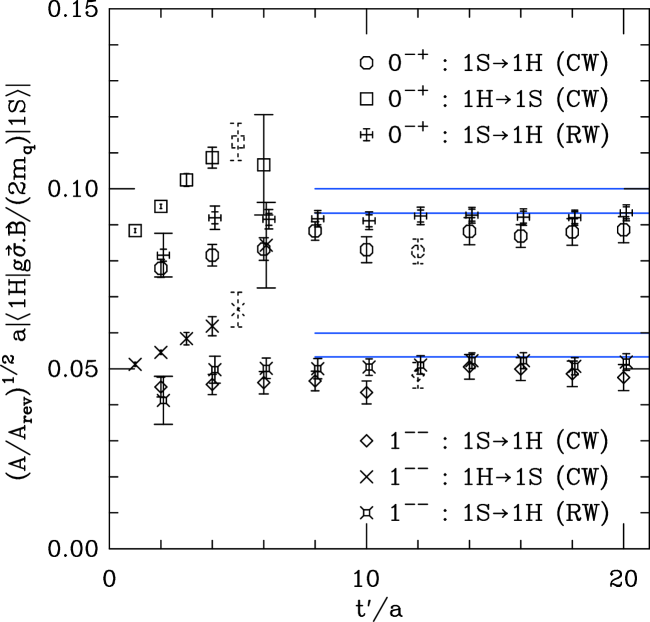
Figure 3: Comparison of the results obtained for the mixing matrix element via the CW source and the RW source with the hybrid mass fixed to that found with the CW hybrid source. The dotted symbols mark the ones used in the geometric mean to get the CW-source results, the $1\sigma$ ranges of which are denoted by the horizontal lines.

Figure 4: The mixing matrix element vs the time of application of the interaction term. CW source, $\beta=7.75$, $am_{q}=3.2$. The dotted symbols mark the ones used in the geometric mean to get the CW-source results.

Figures 4 and 5 display similar plots for the $\beta=7.75$ and 8.4 lattices, respectively. Here we see more convincing plateaus for the matrix element from the hybrid$\rightarrow$S-wave correlators.

Figure 5: The mixing matrix element vs the time of application of the interaction term. CW source, $\beta=8.4$, $am_{q}=1.8$. The dotted symbols mark the ones used in the geometric mean to get the CW-source results.

In Fig. 6 we show the results for one of the lighter masses (around $m_{c}$) for the $\beta=8.0$ lattices. A quick look at the result for the $1^{--}$ channel, however, shows that the non-relativistic approximation (at least at the level of simplicity in our heavy-quark Hamiltonian) may not be such a great idea:

$$\frac{\langle 1H|\delta{\cal H}|1S\rangle}{2m_{q}}\approx\frac{0.14}{1.4}\approx 0.1\sim v^{4}.$$ (23)

The mass required at this lattice spacing to reach the charm quark is also problematic for the expansion ($am_{c}<1$). In spite of these problems we carry on and present our results for charmonium, encouraging the reader not to forget the large systematic effects we introduce by neglecting other terms in our heavy-quark Hamiltonian and by simulating at such a small quark mass.

Figure 6: The mixing matrix element vs the time of application of the interaction term. CW source, $\beta=8.0$, $am_{q}=0.7$. The dotted symbols mark the ones used in the geometric mean to get the CW-source results.

All of the CW-source results for the configuration-mixing matrix elements, along with the corresponding mixing angles, are shown in Tables 4 and 5. The last column displays the final results after an extrapolation (linear) in quark mass to the bottom (or charm) mass determined previously (see Table 3). The hybrid configuration content of the $0^{-+}$ ground state is enhanced by the expected factor of $\sqrt{3}$ (due to spin statistics for single-gluon emission/absorption Barnes (1979); Barnes et al. (1983)) relative to that in the $1^{--}$ channel. Up to this point we have ignored the radiative correction ($c_{B}=1$) and we point out the need for this factor, $c_{B}(a(\beta))$, in the final column. To be precise, this factor should be included in the matrix element, but for small mixing angles, this correction appears as a multiplicative factor in the final result: $\sin\theta\approx\langle 1H|\delta{\cal H}|1S\rangle/(m_{1h}-m_{1s})$.

Table 4: Results for the $1^{--}$ S-wave/hybrid configuration mixing (CW source).

$\beta$	$am_{q}$	$\left|\left\langle 1H\left|a\delta{\cal H}\right|1S\right\rangle\right|$	$|\sin(\theta)|$	$|\langle 1H|\Upsilon\rangle|$
7.75	3.2	0.0624(61)	0.0566(27)	0.058(3)$c_{B}(\beta)$
	3.6	0.0582(61)	0.0518(27)
8.0	2.5	0.0566(33)	0.0618(28)	0.063(3)$c_{B}(\beta)$
	2.8	0.0522(31)	0.0564(27)
8.4	1.8	0.0369(44)	0.0618(36)	0.064(4)$c_{B}(\beta)$
	2.0	0.0352(44)	0.0578(36)
				$|\langle 1H|J/\psi\rangle|$
8.0	0.7	0.1349(84)	0.1483(81)	0.150(8)$c_{B}(\beta)$
	0.8	0.1259(74)	0.1393(70)

Table 5: Results for the $0^{-+}$ S-wave/hybrid configuration mixing (CW source).

$\beta$	$am_{q}$	$\left|\left\langle 1H\left|a\delta{\cal H}\right|1S\right\rangle\right|$	$|\sin(\theta)|$	$|\langle 1H|\eta_{b}\rangle|$
7.75	3.2	0.1032(58)	0.0945(26)	0.097(3)$c_{B}(\beta)$
	3.6	0.0954(57)	0.0862(26)
8.0	2.5	0.0966(34)	0.1031(29)	0.106(3)$c_{B}(\beta)$
	2.8	0.0887(32)	0.0939(27)
8.4	1.8	0.0767(60)	0.1156(52)	0.120(5)$c_{B}(\beta)$
	2.0	0.0723(61)	0.1074(53)
				$|\langle 1H|\eta_{c}\rangle|$
8.0	0.7	0.2327(77)	0.2403(62)	0.243(6)$c_{B}(\beta)$
	0.8	0.2172(69)	0.2270(56)

Meson correlators with the $\vec{\sigma}\cdot\vec{B}$ term applied at all intermediate time slices were also created in order to study the S-wave hyperfine splittings and to attempt to determine $c_{B}(\beta)$. For these, the values of $c_{B}=1$ and 2 were intended; however, a sign error was discovered (much too late) in our field-strength routine which forces us to work with $c_{B}=-1$ and $-2$. (This has no effect upon our configuration-mixing results up to this point since they result from a single application of the spin-dependent term.) The resulting hyperfine splittings for the S-wave states may be found in Table 6.

Table 6: 1S hyperfine splittings.

$\beta$	$am_{q}$	$c_{B}^{2}$	$M_{\Upsilon}-M_{\eta_{b}}$ (MeV)	$c_{B}^{2}(\beta)$
7.75	3.2	1	16.7(1.3)	$(M_{\Upsilon}-M_{\eta_{b}})_{\rm exp}/(17\,{\rm MeV})$
		4	63.6(5.1)
8.0	2.5	1	21.90(55)	$(M_{\Upsilon}-M_{\eta_{b}})_{\rm exp}/(22\,{\rm MeV})$
		4	81.6(2.6)
8.4	1.8	1	25.2(1.1)	$(M_{\Upsilon}-M_{\eta_{b}})_{\rm exp}/(25\,{\rm MeV})$
		4	93.5(4.9)
			$M_{J/\psi}-M_{\eta_{c}}$ (MeV)
8.0	0.7	1	68.0(1.8)	$\approx 1.2-1.7$
		4	213.6(7.1)

Whereas our bottomonium systems seem to follow the $c_{B}^{2}$ proportionality and our charmonium systems do not, there is no experimentally measured mass for the $0^{-+}$ $b\bar{b}$ meson ($\eta_{b}$) while the corresponding $c\bar{c}$ meson ($\eta_{c}$) has been observed. So we report our findings for $c_{B}^{2}(a(\beta))$ from the bottomonium systems in terms of the $M_{\Upsilon}-M_{\eta_{b}}$ mass splitting. For the charmonium results, we report two values for $c_{B}^{2}(\beta)$. The larger value is the result of a linear extrapolation from 0 through the $c_{B}^{2}=1$ point to $M_{J/\psi}-M_{\eta_{c}}=117$ MeV at $c_{B}^{2}=c_{B}^{2}(\beta)$. If we believe the physical quark mass shifts with the inclusion of the spin-dependent term and that this is the dominant effect in explaining why our $c\bar{c}$ hyperfine splitting is not $\propto c_{B}^{2}$, then this is the result we would trust more. If, however, we believe there is a $c_{B}^{3}$ correction present and that this is the dominant effect, we should trust the lower value, which results from using an interpolation of the form $a_{2}c_{B}^{2}+a_{3}c_{B}^{3}$ through the $c_{B}=-1$ and $-2$ points and extrapolating to 117 MeV in the $c_{B}>0$ region. If we use these results with that from $b\bar{b}$ at $\beta=8.0$, we find $M_{\Upsilon}-M_{\eta_{b}}\approx 26-38$ MeV and $c_{B}(\beta=7.75)\approx 1.24-1.50$, $c_{B}(\beta=8.0)\approx 1.09-1.31$, $c_{B}(\beta=8.4)\approx 1.02-1.23$. Any such determination of the radiative corrections, however, is further complicated by the fact that it incorporates systematic effects due to the termination of the NRQCD expansion Trottier (1997); Stewart and Koniuk (2001).

Given our previous worries about our $c\bar{c}$ results ($v^{4}\sim 0.1$; $am_{c}<1$), we may also consider the possible range of $c_{B}$ values using potential model values for the $b\bar{b}$ S-wave hyperfine splittings Chen and Oakes (1996); Yndurain (2001): $\sim 30-60$ MeV. Assuming the $\vec{\sigma}\cdot\vec{B}$ term to dominate this splitting results in $c_{B}(\beta=7.75)\sim 1.33-1.88$, $c_{B}(\beta=8.0)\sim 1.17-1.65$, $c_{B}(\beta=8.4)\sim 1.10-1.55$; or roughly

$$|\langle 1H|\Upsilon\rangle|\sim 0.076-0.11\hskip 5.69046pt;\hskip 5.69046pt|\langle 1H|\eta_{b}\rangle|\sim 0.13-0.19$$

and

$$|\langle 1H|J/\psi\rangle|\sim 0.18-0.25\hskip 5.69046pt;\hskip 5.69046pt|\langle 1H|\eta_{c}\rangle|\sim 0.29-0.4.$$

Each of these ranges lies between two corresponding values (with and without the color Coulomb interaction) determined within the MIT bag model Barnes (1979). The upper limit of the $J/\psi$ result is consistent with that from an adiabatic potential model Gerasimov (1998).

Again, however, the above determinations of $c_{B}(\beta)$ include systematic effects due to the neglect of other terms in the velocity expansion which also contribute to the hyperfine splittings Trottier (1997); Stewart and Koniuk (2001). We are therefore left without precise values for the radiative corrections and may only state that if the $\vec{\sigma}\cdot\vec{B}$ term does in fact dominate the S-wave hyperfine splitting, then these corrections appear to enhance the configuration mixing further.

Figure 7: Hybrid/S-wave configuration mixing angle vs lattice spacing. For each channel, the three lowest points (solid fit line) represent the (tadpole-improved) tree-level results: $c_{B}=1$. The middle three points result from setting the radiative corrections with the S-wave hyperfine splitting held constant at 30 MeV. The uppermost points result from the same splitting set to 60 MeV. The $1^{--}$ points are shifted slightly to the left for clarity.

In Fig. 7 we plot our results for the bottomonium configuration-mixing angle as a function of the lattice spacing. The plot includes the tree-level results, along with two others altered using radiative corrections given by assumed values for the S-wave hyperfine splitting due to the $\vec{\sigma}\cdot\vec{B}$ term. Some positive features may be noted in this plot. First, the choice of the “physical” value for the hyperfine splitting does not seem to have a large effect upon the scaling displayed by the points (however, the values at any one lattice spacing are greatly affected). Also, at least for the $0^{-+}$ channel, the fixing of the hyperfine splittings appears to slightly improve the scaling; the tree-level and radiatively-corrected values for the $1^{--}$ appear to scale equally well.

For the bottomonium systems on our lattices, where we have $a\gtrsim 1/m_{b}$, discretization effects are expected to be about the same order as those due to the relativistic corrections we neglect. In Ref. Lepage et al. (1992), a prescription for removing such systematics by improving the heavy-quark action has been presented. Such improvements are not included in this current work and therefore discretization effects may also be partly responsible for the trends seen in the tree-level results of Fig. 7 (for the $0^{-+}$ channel, $\sim$20% rise in the central value by cutting the lattice spacing in half; $\sim$10% for the $1^{--}$).

IV Conclusions

We have determined the relative contribution of the lowest hybrid configuration to the wavefunctions of heavy S-wave mesons. Our approach utilizes the non-relativistic approximation to lattice QCD, applicable for heavy quarkonia where there is a clear separation of radial, orbital, and gluonic excitations and the mixing among the corresponding configurations is small.

Tadpole-improved, tree-level results ($c_{B}=1$ in Tables 4 and 5) display hybrid configuration admixtures at about $(0.063)^{2}\approx 0.4$% probability within the $\Upsilon$ and about $(0.15)^{2}\approx 2.3$% for $J/\psi$. The corresponding results for the pseudoscalar channels are enhanced by $\approx 3$ due to spin statistics Barnes (1979); Barnes et al. (1983).

Although the radiative corrections for the spin-dependent term in our heavy-quark Hamiltonian elude evaluation, these factors may provide further enhancement of the configuration mixing.

Quenching appears to significantly affect the lattice spacing results (see Table 2 and Ref. Bernard et al. (2000)), decreasing those determined via bottomonium mass splittings (by perhaps 10%, see Ref. Burch (2003)). This, in turn, affects the quark mass extrapolation and the determination of the radiative correction, but the direct effect upon the configuration mixings is not clear. This may only be answered by repeating the analysis on lattices with dynamical quarks.

Inclusion of higher-order terms within the NRQCD Hamiltonian has been shown to alter bottomonium hyperfine splittings significantly (by as much as 15% in one case Trottier (1997)). In principle, such terms can cause the same configuration mixings as those determined here through only the $\vec{\sigma}\cdot\vec{B}$ term and may be needed to achieve a more accurate measure of the hybrid configuration content within the $\Upsilon$ and $\eta_{b}$. The situation for our charmonium results is more dire. For these systems, the heavy-quark expansion can hardly be trusted on our lattices ($am_{c}<1$) and higher-order corrections may contribute as much or more to the mixing.

These results have implications for theoretical determinations of certain quarkonium quantities. For example, since the $J/\psi\rightarrow e^{+}e^{-}$ decay should not occur directly from the hybrid configuration Barnes (2003b), our results suggest about a $(0.15)^{2}\approx 2.3(2)$% suppression of the $\Gamma(J/\psi\rightarrow e^{+}e^{-})$ partial width determined via potential models; about a $(0.063)^{2}\approx 0.40(4)$% suppression for $\Gamma(\Upsilon\rightarrow e^{+}e^{-})$. These effects appear to be rather small (the corresponding experimental errors lie at about 7% and 4% for $J/\psi$ and $\Upsilon$, respectively Hagiwara et al. (2002)) and this analysis lends support to their neglect thus far, at least for the $\Upsilon$, where our lattice heavy-quark expansion is more trustworthy.

The other side to this issue is that of the vector hybrid states containing some admixture of the $q\bar{q}$ vector configurations and therefore coupling to $e^{+}e^{-}$. The above (tree-level) results would suggest the appearance of a $c\bar{c}g$ hybrid resonance with a partial width of

$$\Gamma(c\bar{c}g\rightarrow e^{+}e^{-}) \approx 0.023(2)\times\Gamma(J/\psi\rightarrow e^{+}e^{-})$$

$$\approx 0.12(1)\,{\rm keV}$$

somewhere around $E_{cm}=M_{c\bar{c}g}\approx 4.4-4.7$ GeV (the lower estimate arises from using the $r_{1}$-determined value of the lattice spacing) and a $b\bar{b}g$ hybrid resonance with

$$\Gamma(b\bar{b}g\rightarrow e^{+}e^{-}) \approx 0.0040(4)\times\Gamma(\Upsilon\rightarrow e^{+}e^{-})$$

$$\approx 0.0053(5)\,{\rm keV}$$

around $M_{b\bar{b}g}\approx 10.8-11.1$ GeV. Any such $b\bar{b}g$-dominated resonance should thus be extremely difficult to see in $e^{+}e^{-}$ $R$-scans given this very small partial width and (most likely) much larger overall width. The $c\bar{c}g$-dominated state gives a partial width of the same order of that seen in a resonance within the same mass range: $\psi(4415)$ with $\Gamma(e^{+}e^{-})=0.47(10)$ keV Hagiwara et al. (2002); Siegrist et al. (1976); Brandelik et al. (1978); $\psi(4430)$ with $\Gamma(e^{+}e^{-})=0.390(74)$ keV from Refs. Bai et al. (2002); Eidemuller (2002). However, this hardly qualifies as evidence of a hybrid-dominated structure for such a resonance. Our charmonium results are plagued with systematic errors which are not easily quantified (given the charm quark mass and lattice spacings we use, the mixing through other terms in the expansion of the heavy-quark Hamiltonian may be even larger). Besides, any such determination would not only require a study of the possible decays from the hybrid state (determining the total width), but would also need to consider mixings of the $c\bar{c}g$ configuration with other $c\bar{c}$ configurations which lie closer in mass. The use of lattices with a finer temporal resolution may be helpful in resolving multiple states in future simulations.