CERN-TH/2003-62

DESY 03-029

Reducing Residual-Mass Effects for Domain-Wall Fermions

Karl Jansen^a and Kei-ichi Nagai^b

^aNIC/DESY Zeuthen, Platanenallee 6, D-15738 Zeuthen, Germany

^bCERN, Theory Division, CH-1211 Geneva 23, Switzerland

It has been suggested to project out a number of low-lying eigenvalues of the four-dimensional Wilson–Dirac operator that generates the transfer matrix of domain-wall fermions in order to improve simulations with domain-wall fermions. We investigate how this projection method reduces the residual chiral symmetry-breaking effects for a finite extent of the extra dimension. We use the standard Wilson as well as the renormalization–group–improved gauge action. In both cases we find a substantially reduced residual mass when the projection method is employed. In addition, the large fluctuations in this quantity disappear.

1 Introduction

Domain-wall fermions (DWF) preserve chiral symmetry [1, 2, 3] when the lattice size in the 5th direction, $N_{s}$, is taken to infinity. The approach to the chiral limit is exponential in $N_{s}$, with a rate given by the eigenvalues of the transfer matrix along the 5th direction, which is a local operator in 4 dimensions [4, 5, 6, 7]. A measure of chiral symmetry breaking, taking place for finite $N_{s}$, is the residual mass, $m_{\mathrm{res}}$, derived from the axial Ward–Takahashi identity.

Even if the restoration of chiral symmetry is expected to be exponentially fast in $N_{s}$, in practice $m_{\mathrm{res}}$ can decrease very slowly as first shown by the CP–PACS collaboration [8, 9]. The slow convergence of the residual mass is due to the existence of very small eigenvalues of the four-dimensional operator defining the transfer matrix along the 5th direction. In particular, at large $N_{s}$ these low-lying modes dominate the convergence rate [9] and render the recovery of chiral symmetry difficult. Even if the residual mass is very small, it is then not clear whether and what distortions of chiral symmetry are still present. Since large numerical simulations with DWF are being performed (see e.g. refs. [8, 10] and the reviews [11, 12]) it becomes important to find ways around this obstacle. Such solutions for improving the chiral properties of DWF then have to come from eliminating these low-lying modes.

One idea to reduce these small eigenvalues is the improvement of the gauge actions [8, 9, 10, 13] such as Iwasaki [14] or DBW2 [15]. However, besides the potential difficulties with unitarity violations [16] and the sampling problems of topological charge sectors [17], this method does not solve the problem completely. For example, with the Iwasaki gauge action, the convergence rate also becomes slow at large $N_{s}$ [9]. The reason is that again very small eigenvalues of the transfer matrix appear in this case, though less frequently than for the Wilson gauge action. Using the DBW2 gauge action seems to be much better in this respect [10, 17], but it is unclear whether these small eigenvalues could eventually appear there, too, leading to similar problems. A perturbative analysis [18] suggests a modification of the four-dimensional component of the domain wall operator to tackle the problem. This is, however, not yet tested in simulations.

Another method to eliminate the disturbing effect of the small eigenvalues and the corresponding set of eigenstates of the transfer matrix is to project them out and lift them in a way that does not change the $N_{s}\rightarrow\infty$ limit of the DWF operators [19, 20]. In this paper, we investigate the projection method based on ref. [19], where the projection is performed in the transfer matrix itself. In ref. [20], an alternative projection is implemented through a modification of the boundary terms. The philosophy of both approaches is the same as the one using the transfer matrix. The aim of this article is to investigate the effects of the projection method on the residual mass in quenched simulations. As we will see, the projection method works very well, leading to a substantial improvement in the residual mass.

Let us emphasize that simulations with DWF can be considered under two aspects. The “purist’s” approach demands exact chiral symmetry at non-zero lattice spacing. Here any violation of chiral symmetry (in practice up to machine precision) is not tolerable. Hence the value of $N_{s}$ is to be taken as large as possible and the additive mass renormalization $m_{\mathrm{res}}\neq 0$ has to be eliminated. Thus the projection method discussed here, or any method leading to the same improvement, becomes an unavoidable necessity in this case. A different, more practical point of view is to consider DWF at finite, and even small, values of $N_{s}$ as a highly improved Wilson fermion. Also in this case, the projection method will accelerate the numerical simulation considerably and should therefore be employed.

2 Domain-wall fermions and Ward–Takahashi identity

In this section, we establish our notation and give the Ward–Takahashi identity in order to define the residual mass. For completeness, we give here the definition of the domain-wall operator and its relation to the 4D operator satisfying the Ginsparg–Wilson equation [21]. We follow the presentation of [19]. Derivations of this formulae can be found in [2, 3, 4, 5, 7]. The 5D domain-wall operator is defined as

$${\cal D}={1\over 2}\left\{\gamma_{5}\left(\partial^{*}_{s}+\partial_{s}\right)-a_{s}\partial^{*}_{s}\partial_{s}\right\}+{\cal M}\quad,$$ (2.1)

where $s$ denotes a lattice site in the 5th direction ($1\leq s\leq N_{s}$), $a_{s}$ is the corresponding lattice spacing, and $\partial^{*}_{s}$ and $\partial_{s}$ are the free forward and backward derivatives.

The operator ${\cal M}$ is obtained from the standard 4D Wilson–Dirac operator by

$${\cal M}=D_{W}-m_{0}$$ (2.2)

with

$$D_{W}={1\over 2}\left\{\gamma_{\mu}\left(\nabla^{*}_{\mu}+\nabla_{\mu}\right)-a\nabla^{*}_{\mu}\nabla_{\mu}\right\}\quad.$$ (2.3)

Here $\nabla^{*}_{\mu}$ and $\nabla_{\mu}$ are the gauge covariant forward and backward derivatives and $a$ is the lattice spacing in the four physical dimensions $\mu=1,\dots,4$. The domain-wall parameter $m_{0}$ obeys

$$0<a_{s}m_{0}<2\quad,\quad 0<am_{0}<2\quad.$$ (2.4)

Note that the lattice spacings $a_{s}$ and $a$ can be different in general. The boundary conditions in the DWF formulation in the 5th direction is

$$P_{+}\psi(0,x)=P_{-}\psi(N_{s}+1,x)=0\quad,$$ (2.5)

where $P_{\pm}\equiv{1\over 2}(1\pm\gamma_{5})$. In these settings, the chiral modes with opposite chiralities are localized on 4D boundary planes at $s=1$ and $s=N_{s}$.

The 4D quark fields are constructed from the left and right boundary (chiral) modes, as follows:

$$q(x)=P_{-}\psi(1,x)+P_{+}\psi(N_{s},x)\quad,\quad\bar{q}(x)=\bar{\psi}(1,x)P_{+}+\bar{\psi}(N_{s},x)P_{-}\quad.$$ (2.6)

A bare quark mass term is introduced by adding to eq. (2.1) the term

$$m_{f}\left\{\bar{\psi}(1,x)P_{+}\psi(N_{s},x)+\bar{\psi}(N_{s},x)P_{-}\psi(1,x)\right\}=m_{f}\bar{q}(x)q(x)\quad.$$ (2.7)

The propagator of the quark fields is related to an effective 4D operator $D_{N_{s}}$ [4, 5, 7]

$$\langle q(x)\bar{q}(x)\rangle=\frac{2-aD_{N_{s}}}{aD_{N_{s},m_{f}}}\quad,$$ (2.8)

with

$$D_{N_{s},m_{f}}=\left(1-am_{f}\right)D_{N_{s}}+2m_{f}\quad.$$ (2.9)

In terms of the operators $K_{\pm}$,

$$K_{\pm}\equiv{1\over 2}\pm{1\over 2}\gamma_{5}\frac{a_{s}{\cal M}}{2+a_{s}{\cal M}}\quad,$$ (2.10)

$D_{N_{s}}$ is given by

$$aD_{N_{s}}=1+\gamma_{5}\frac{K_{+}^{N_{s}}-K_{-}^{N_{s}}}{K_{+}^{N_{s}}+K_{-}^{N_{s}}}\quad.$$ (2.11)

From this equation, it is easy to show that

$$aD\equiv\lim_{N_{s}\rightarrow\infty}aD_{N_{s}}=1+\gamma_{5}\,{\rm sign}\left(K_{+}-K_{-}\right)\quad,$$ (2.12)

which is written as

$$aD=1-\frac{A}{\sqrt{A^{\dagger}A}}\quad,$$ (2.13)

$$A=-\frac{a_{s}{\cal M}}{2+a_{s}{\cal M}}\quad.$$ (2.14)

The operator $D$ in eq. (2.13) satisfies the Ginsparg–Wilson relation. The only difference to Neuberger’s operator [22] is the definition of $A$. Neuberger’s operator is obtained from eqs. (2.13) and (2.14) by taking the limit $a_{s}\rightarrow 0$.

In the limit $N_{s}\rightarrow\infty$, the 5D formulation of DWF is completely equivalent to a 4D lattice formulation of Ginsparg–Wilson fermions satisfying an exact chiral symmetry. However, in a realistic simulation $N_{s}$ is kept finite, of course. In this situation, the chiral symmetry is explicitly broken by the residual terms $\delta D\equiv D_{N_{s}}-D$. A measurement of the effects of this chiral symmetry breaking is the so-called residual mass $m_{\mathrm{res}}$, derived from the axial Ward–Takahashi identity. The chiral transformation of DWF is defined as

$$\delta\psi(s,x)=iQ(s)\epsilon\psi(s,x)\,,\,\quad\delta\bar{\psi}(s,x)=-i\bar{\psi}(s,x)Q(s)\epsilon\,,$$ (2.15)

where $Q(s)={\rm sign}(N_{s}-2s+1)$ and $\epsilon$ is an infinitesimal transformation parameter. Under this transformation, the quark fields are transformed as the usual chiral transformation: $\delta q(x)=i\gamma_{5}\epsilon q(x)\,,\,\delta\bar{q}(x)=i\bar{q}(x)\gamma_{5}\epsilon$ . Therefore the axial Ward–Takahashi identity is

$$\sum_{\mu}\langle\nabla_{\mu}A_{\mu}(x)P(0)\rangle=2m_{f}\langle P(x)P(0)\rangle+2\langle J_{5q}(x)P(0)\rangle\quad,$$ (2.16)

where $A_{\mu}(x)$ is the axial-vector current and $P(x)$ is the pseudo-scalar density; $A_{\mu}(x)$ and $P(x)$ are given as

$$A_{\mu}(x)=\sum_{s}Q(s)J_{\mu}(s,x)\quad,\quad P(x)=\bar{q}(x)\gamma_{5}q(x)\quad,$$ (2.17)

where

$$J_{\mu}(x)=\frac{1}{2}\left[\bar{\psi}(s,x)(1-\gamma_{\mu})U_{\mu}(x)\psi(s,x+\mu)-\bar{\psi}(s,x+\mu)(1+\gamma_{\mu})U^{\dagger}_{\mu}(x)\psi(s,x)\right]\quad.$$ (2.18)

The additional term $J_{5q}$ represents the explicit breaking of chiral symmetry,

$$J_{5q}=-\bar{\psi}\left(\frac{N_{s}}{2},x\right)P_{-}\psi\left(\frac{N_{s}}{2}+1,x\right)+\bar{\psi}\left(\frac{N_{s}}{2}+1,x\right)P_{+}\psi\left(\frac{N_{s}}{2},x\right)\quad.$$ (2.19)

For a smooth gauge field background, the term $\langle J_{5q}P\rangle$ vanishes exponentially fast [3, 6, 23] as $N_{s}$ is increased. In realistic simulations, however, the gauge fields can be rough and it may happen that the rate of convergence in $N_{s}$ is rather poor. The breaking of chiral symmetry can be quantified by the values of $m_{\mathrm{res}}$. Let us define the ratio $R(t)$:

$$R(t)=\frac{\sum_{\bf x}\langle J_{5q}({\bf x},t)P({\bf 0},0)\rangle}{\sum_{\bf x}\langle P({\bf x},t)P({\bf 0},0)\rangle}\quad.$$ (2.20)

The usual definition of $m_{\mathrm{res}}$ is the average of the quantity $R(t)$ at large time separations. A necessary but, maybe, not sufficient condition to recover fully on-shell chiral symmetry at a non-vanishing value of the lattice spacing is that this quantity be negligible.

3 Eigenvalues of $A^{\dagger}A$

For gauge configurations with a restricted value of the plaquette (so-called admissible configurations) [6, 23], the operator $A^{\dagger}A$ has been shown to have a spectral gap, $0<u\leq A^{\dagger}A\leq v$, ensuring the exponential suppression of the residual mass in $N_{s}$. However, in realistic simulations as performed today, the plaquette bound is not satisfied and it is important to study the distribution of the eigenvalues of $A^{\dagger}A$ in numerical simulations.

The eigenvalues of $A^{\dagger}A$ can be obtained through the generalized 4D eigenvalue equation [24]

$$a_{s}^{2}{\cal M}^{\dagger}{\cal M}\psi=\lambda\,\,(2+a_{s}{\cal M})^{\dagger}(2+a_{s}{\cal M})\psi\quad.$$ (3.1)

The low-lying (maximal) eigenvalues can be computed by minimizing (maximizing) the generalized Ritz functional

$$\frac{\langle\psi|a_{s}^{2}{\cal M}^{\dagger}{\cal M}|\psi\rangle}{\langle\psi|(2+a_{s}{\cal M})^{\dagger}(2+a_{s}{\cal M})|\psi\rangle}$$ (3.2)

using a straightforward generalization of the algorithm described in ref. [25]. Notice that in this method no inversion of the matrix $(2+a_{s}{\cal M})^{\dagger}(2+a_{s}{\cal M})$ is needed. Higher eigenvalues can be calculated by modifying the operator ${\cal M}^{\dagger}{\cal M}$ in the numerator in eq. (3.2), so that the already computed eigenvalues are shifted to larger values. This can be achieved [19] by substituting

$${\cal M}^{\dagger}{\cal M}\rightarrow{\cal M}^{\dagger}{\cal M}+\sum_{i}\left(\frac{1-\lambda_{i}}{\lambda_{i}}\right){\cal M}^{\dagger}{\cal M}|\psi_{i}\rangle\langle\psi_{i}|(2+a_{s}{\cal M})^{\dagger}(2+a_{s}{\cal M})\,,$$ (3.3)

$\lambda_{i}$, $\psi_{i}$ being the already computed (lower) eigenvalues and eigenvectors.

Figure 1 shows the eleven lowest eigenvalues of the operator $A^{\dagger}A$ as a function of the Monte Carlo time ($t_{\mathrm{MC}}$). Here and throughout the paper we use the quenched approximation and set $a_{s}=1$. The data in Fig. 1 are obtained with the Wilson gauge action at $\beta=6.0$ on a $12^{3}\times 24$ lattice, setting $m_{0}=1.8$. As expected, very small eigenvalues appear frequently.

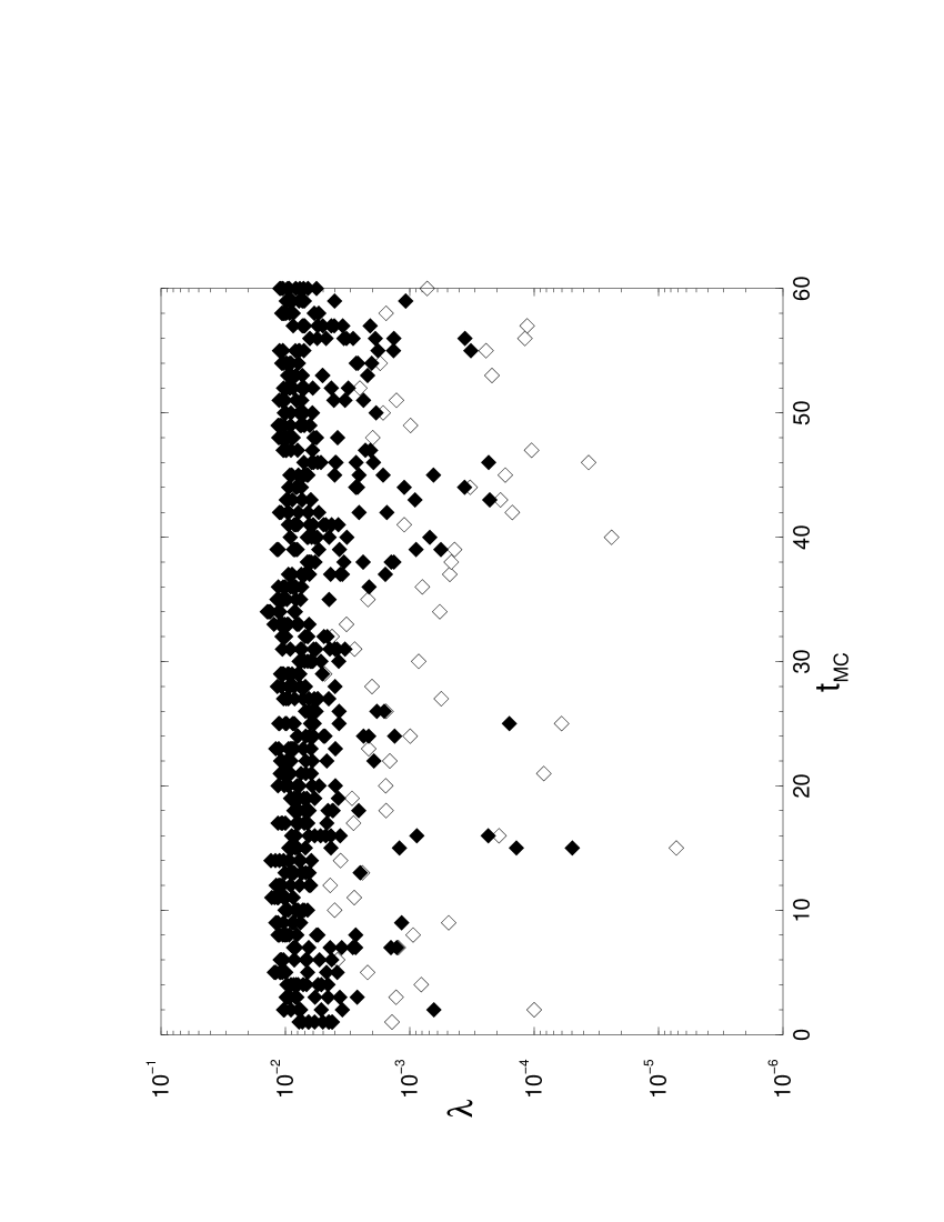
Figure 1: The 11 lowest eigenvalues of the operator $A^{\dagger}A$ as a function of Monte Carlo time $t_{\mathrm{MC}}$ at $\beta=6.0$ and $m_{0}=1.8$ on a $12^{3}\times 24$ lattice. The open diamonds denote the lowest eigenvalue.

The minimum rate of convergence in $N_{s}$ of the operator $D_{N_{s}}$ is given by

$$\omega=\min_{i}[\omega_{i}]\quad,\quad\omega_{i}\equiv\ln\frac{1+\sqrt{\lambda_{i}}}{|1-\sqrt{\lambda_{i}}|}\quad,$$ (3.4)

where $\lambda_{i}$ are the eigenvalues of $A^{\dagger}A$ [19]. Figure 2 shows the inverse convergence rate computed from the eigenvalues in Fig. 1. Clearly, the low-lying eigenvalues of $A^{\dagger}A$ lead to a slow convergence, causing the simulation to become expensive.

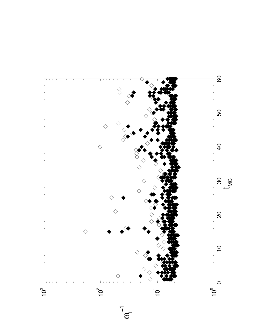
Figure 2: The inverse convergence rate $\omega_{i}^{-1}$ computed from the eigenvalues plotted in Fig 1.

We also explored the eigenvalues for other gauge actions such as the Iwasaki [14] and DBW2 [15] ones. An example for these eigenvalues is plotted in Fig. 3. In that figure we average over 20 gauge configurations. The parameters of the gauge actions were chosen such that in each case the value of the lattice spacing is $a=0.093$ fm, leading to setting $\beta=6.0$ for the Wilson action, $\beta=2.6$ for the Iwasaki one and $\beta=1.04$ for the DBW2 one. Since also the lattice size was fixed to be $12^{3}\times 24$ we have for the different gauge actions the same physical situation. For the Wilson action we observe small values for the lowest-lying modes. This is improved substantially by employing the Iwasaki action and even more when using the DBW2 action. Note that the 11th low-lying eigenvalue of the Wilson action corresponds to the lowest eigenvalue of the Iwasaki action. We checked for the Wilson and the Iwasaki action that this picture does not change when we decrease the value of the lattice spacing down to $a=0.05$ fm. This confirms that the convergence in $N_{s}$ is faster when the gauge action is improved [8, 10, 13]. As we will see below a conclusion that improved gauge actions by themselves would completely cure the problem of a slow convergence rate is premature, however.

Figure 3: Averaged eigenvalues for the Wilson, Iwasaki and DBW2 gauge actions as a function of the eigenvalue number. The lattice spacing $a=0.093$ fm used is the same for all gauge actions.

4 Improvement of domain-wall fermion

The decay rate of the residual mass in $N_{s}$ is controlled by the small eigenvalues of $A^{\dagger}A$. For the Wilson gauge action very small eigenvalues occur, leading to a slow convergence. Although the situation is improved for the Iwasaki gauge action, as we saw above, it was observed that even in this case for large values of $N_{s}$ the convergence turned to become very slow [8, 9]. It thus seems to be necessary to test methods as proposed in [19] that modify the fermionic part of the DWF action by projecting out the small eigenvalues of $A^{\dagger}A$. These methods can be used alternatively –or even in addition– to employing improved gauge actions. The key observation in [19] is that the relations in eqs. (2.13) and (2.14) hold true for any choice of ${\cal M}$ as long as

$${\cal M}^{\dagger}=\gamma_{5}{\cal M}\gamma_{5}\quad,\quad\det(2+a_{s}{\cal M})\neq 0\quad.$$ (4.1)

This fact may be used to construct an improved ${\cal M}$ for which the very low eigenvalues of $A^{\dagger}A$ disappear.

Let us, for completeness, repeat the construction of the improved operator here again following [19]. The basic idea is to find the new operator ${\widehat{\cal M}}$ satisfying the following relation;

$$\widehat{A}=-\frac{a_{s}\widehat{\cal M}}{2+a_{s}{\widehat{\cal M}}}=A+\sum_{k=1}^{r}(\widehat{\alpha}_{k}-\alpha_{k})\gamma_{5}v_{k}\otimes v_{k}^{\dagger}\quad,$$ (4.2)

where $v_{k}$ is the eigenvector of the following equation

$$\gamma_{5}Av_{k}=\alpha_{k}v_{k}\quad,\quad k=1,\dots,r\quad,\quad(v_{k},v_{l})=\delta_{kl}\quad.$$ (4.3)

Therefore an improved DWF operator, $D_{\mathrm{dwf}}^{\mathrm{imp}}$, can be obtained from eq. (2.1) after substituting ${\cal M}$ with $\widehat{\cal M}$ defined as

$$a_{s}\widehat{\cal M}=a_{s}{\cal M}-\sum_{k,l=1}^{r}X_{kl}w_{k}\otimes w_{l}^{\dagger}\gamma_{5}\quad,$$ (4.4)

where

$$w_{k}=(2+a_{s}{\cal M})\gamma_{5}v_{k}$$ (4.5)

and

$$(X^{-1})_{kl}=2\delta_{kl}(\widehat{\alpha}_{k}-\alpha_{k})^{-1}+(v_{k},w_{l})\quad.$$ (4.6)

It is easy to see that $\gamma_{5}\widehat{A}$ has the same eigenvectors as $\gamma_{5}A$; however, all eigenvalues $\alpha_{k}$, $k=1,\dots,r$, are replaced by ${\widehat{\alpha}}_{k}$. The limit $N_{s}\rightarrow\infty$ of $D_{N_{s}}$ is of course unchanged by this modification, provided

$${\rm sign}({\widehat{\alpha}}_{k})={\rm sign}(\alpha_{k})\,.$$ (4.7)

The choice of $|{\widehat{\alpha}}_{k}|$ is not unique. We will choose here

$${\widehat{\alpha}}_{k}=2\;{\rm sign}(\alpha_{k})|\alpha_{l}|\,,\quad 1\leq k\leq r\equiv k_{\mathrm{max}}\,,$$ (4.8)

where $k_{\mathrm{max}}$ is the number of eigenvalues projected out and $l$ can be chosen freely. A natural choice is $l=k_{\mathrm{max}}$ such that all low-lying eigenvalues are moved to be twice higher than the largest eigenvalue projected out. We also tried, however, different values of $l$ and found that the improvement is not very sensitive to the precise choice of ${\widehat{\alpha}}_{k}$, provided it is larger than $\alpha_{k_{\mathrm{max}}}$.

Our statistics is typically $60$ configurations for the Wilson gauge action and $20$ configurations for the Iwasaki action. We did not explore the DBW2 action extensively. The parameters of the gauge actions were chosen as before such that $a^{-1}=2$ GeV, which means a choice of $\beta=6.0$ for the Wilson gauge action and $\beta=2.6$ for the Iwasaki one. The lattice sizes were $12^{3}\times 24\times N_{s}$ and $16^{3}\times 24\times N_{s}$ for the two actions, respectively. The domain-wall mass was $m_{0}=1.8$ and we worked at a quark mass of $m_{f}=0.02$.

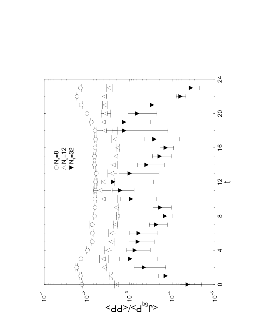
Figure 4: The ratio $R(t)=\frac{\langle J_{5q}P\rangle}{\langle PP\rangle}$ as a function of Euclidean time. The Wilson gauge action is chosen with simulation parameters as given in the text. No projection of eigenvalues is performed.

We have measured the residual mass from $R(t)$ in eq. (2.20) as the average of $R(t)$ for $t$ typically in the interval $4\leq t\leq 20$ for a time extent of the lattice of $T=24$. $R(t)$ is shown in Fig. 4 for the case when no projection is performed. For each value of $N_{s}$ we have the same statistics. Although, with increasing $N_{s}$, the residual mass $m_{\mathrm{res}}$ decreases, it does so rather slowly; furthermore, as $N_{s}$ increases, large fluctuations in $R(t)$ occur, rendering the determination of the residual mass difficult. These large fluctuations also suggest that the residual chirality-breaking effects in other quantities might be very hard to estimate, taking only $m_{\mathrm{res}}$ as a measure of these effects.

In Fig. 5 we show $R(t)$ when we project out a number of eigenvalues. As expected, the projection of the low eigenvalues decreases the residual mass significantly with respect to Fig. 4.

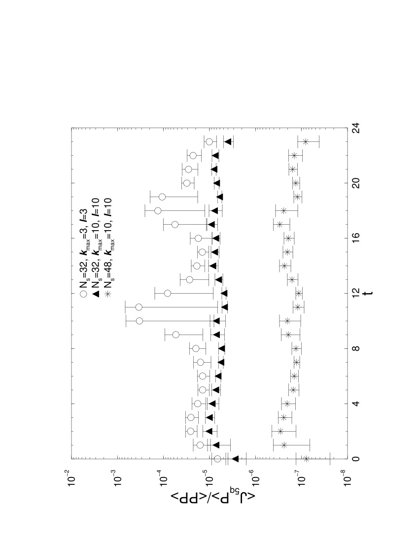
Figure 5: Same as Fig. 4 but now with the projection of eigenvalues employed.

The more eigenvalues are projected the smaller the residual mass is. Another important feature is that the fluctuations in $R(t)$ become much smaller when a sufficiently large number of eigenvalues is projected out; in this case 10 seems to be a good choice. This is very clearly seen in Fig. 6, where we show the value of the ratio $\widehat{R}(t)$,

$$\widehat{R}(t)=\frac{\sum_{\bf x}J_{5q}({\bf x},t)P({\bf 0},0)}{\sum_{\bf x}P({\bf x},t)P({\bf 0},0)}\quad,$$ (4.9)

computed on single configurations at $t=12$ as a function of Monte Carlo time. The spikes are substantially damped with the projection.

Figure 6: The quantity $\widehat{R}(t)-\langle\widehat{R}(t)\rangle$ at $t=12$, see eq. (4.9), as a function of Monte Carlo time for the Wilson gauge action, with and without projection.

Finally, when the projection is implemented, the decrease of the residual mass with $N_{s}$ is much faster.

In summary, it is clear that the projection method has a drastic effect on the value and dispersion of the residual mass. However a sufficient ($O(10)$ in our setup) number of eigenvalues have to be projected out.

5 DWF with improved gauge actions

In our simulations with the Iwasaki gauge action we found, even in our small sample of only 20 configurations, very low-lying eigenvalues of $A^{\dagger}A$. In order to see the effect of these modes we plot, in Fig. 7, the ratio $\widehat{R}(t)$ of eq. (4.9), for two of these configurations (note that no averaging is involved here). The figures indicate that we will find, also for the Iwasaki gauge action, the same problem as for the Wilson gauge action. When no projection is performed, the correlation function shows a spiky behaviour, which may lead to large fluctuations in $\widehat{R}(t)$ and hence to a very difficult determination of the residual mass. This is also confirmed in the ratio of averaged values, $R(t)$, as shown in Fig. 8. The pattern resembles the case of the Wilson gauge action. For small values of $N_{s}$ the effect of the projection is not noticeable. For larger values of $N_{s}$, we see that $R(t)$ is lowered when the eigenvalues are projected out and that the fluctuations of this quantity are strongly damped.

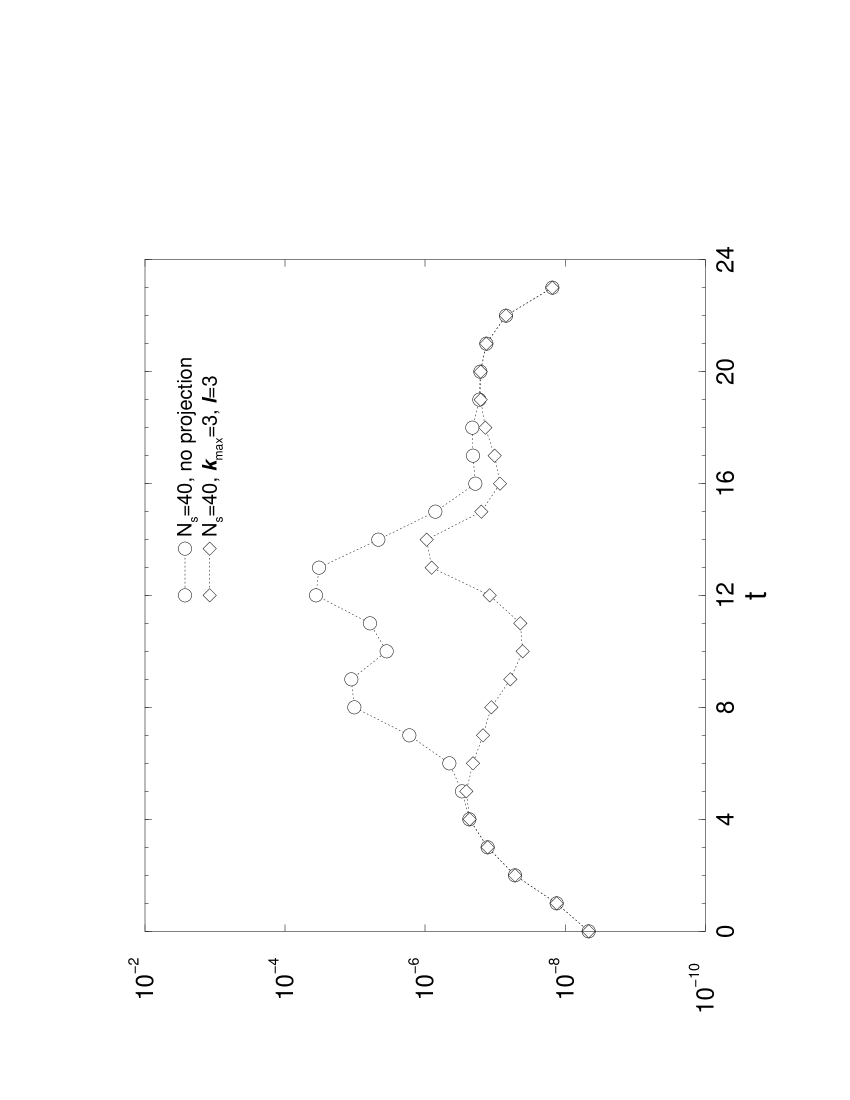
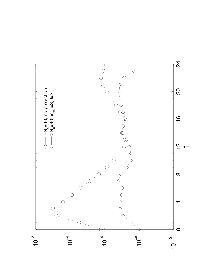
Figure 7: $\widehat{R}(t)$ as a function of time in the Iwasaki action. The circles show the results for the no-projection case and the diamonds for the case when 3 eigenvalues are projected out.

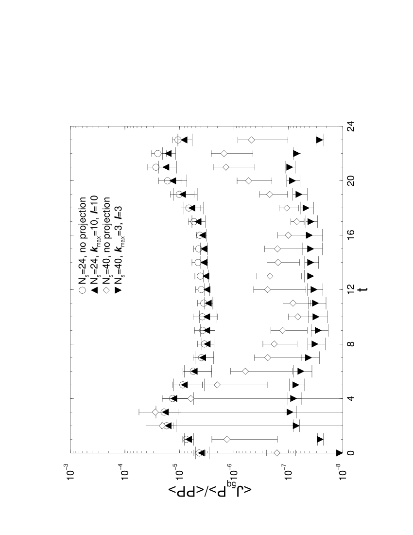
Figure 8: $\frac{\langle J_{5q}P\rangle}{\langle PP\rangle}$ without and with projection for the Iwasaki gauge action.

We also made an attempt to see how the projection method affects $R(t)$ for the DBW2 action. For the simulations we chose $\beta=1.04$, which corresponds again to $a^{-1}=2$ GeV. Thus we study the same physical situation with the Wilson and Iwasaki gauge actions. The lattice size was chosen to be $16^{3}\times 32\times N_{s}$ and $m_{0}=1.7$. The fermion mass was taken to be $m_{f}=0.02$.

We observe in Fig. 9 that the residual mass is not changed very much by the projection. We attribute this to the fact that in our small statistical sample no very low-lying eigenvalues of $A^{\dagger}A$ could be detected. We see, however, from the same figure that the statistical error is substantially reduced for certain values of $t$ when the projection of eigenvalues is employed.

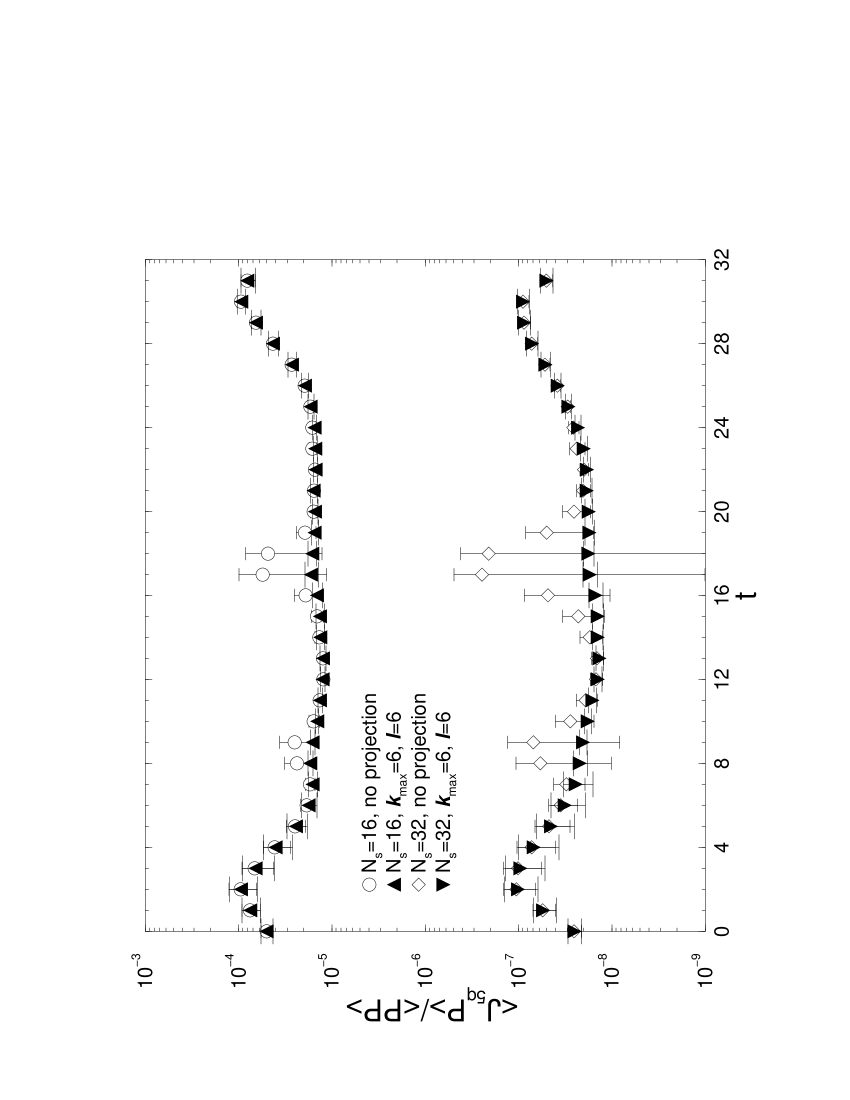
Figure 9: $\frac{\langle J_{5q}P\rangle}{\langle PP\rangle}$ without and with projection at $N_{s}=16$ and 32, for the DBW2 gauge action.

The fact that $R(t)$ shows large fluctuations, even though there are no very small low-lying eigenvalues, points toward the suspicion that also the eigenvectors may play an important role. In particular the localization properties of these eigenmodes may lead to large fluctuations as discussed in [26]. Although this point deserves further investigation, we did not perform such a study here. To conclude, from a negligible average value of the residual mass, that chiral symmetry is restored is certainly questionable when the dispersion of the residual mass is large and not gaussian. A much safer situation would be to ensure that the residual mass is bounded from above for all configurations. The projection method ensures that this is the case.

To summarize, in Fig. 10 we show the comparison of the behaviour of the residual mass as a function of $N_{s}$ for different gauge actions and for different numbers of projected eigenvalues. For a fixed gauge action, we find that at small $N_{s}$ there is almost no effect from the projection method.

This can be explained by a simple qualitative argument with the formula suggested in [18, 9, 26];

$$m_{\mathrm{res}}\sim\sum_{k}e^{-\alpha_{k}N_{s}}\sim\int d\alpha\rho(\alpha)e^{-\alpha N_{s}}\quad,$$ (5.1)

where $\rho(\alpha)$ is the eigenvalue density in the continuum. This (qualitative) formula describes the behaviour of $m_{\mathrm{res}}$ as a function of $N_{s}$. The formula contains two factors, the eigenvalue density and the exponential supression factor $e^{-\alpha N_{s}}$. For small values of $N_{s}$, not only do the low-lying modes contribute to the sum in eq. (5.1), but also the bulk modes since they are not supressed sufficiently. When projecting out a few number of low-lying eigenmodes, the eigenvalue density and the exponential factor remain almost unchanged and hence also the residual mass is not affected very much for small values of $N_{s}$. In such a case, it would be necessary to project out a large number of eigenmodes to make $m_{\mathrm{res}}$ decrease. When $N_{s}$ is chosen to be large, on the other hand, the bulk mode contributions to the sum in eq. (5.1) will die out and only the small eigenvalue contributions will survive. As a consequence, the factor $e^{-\alpha N_{s}}$ becomes much smaller after projecting out even only a few low-lying (isolated) eigenmodes. This should hence lead to a large improvement, i.e. a substantial decrease of the residual mass when the projection method is active. As Fig. 10 clearly shows, this is indeed the case. For the Wilson gauge action at $N_{s}=48$, the value of the residual mass is decreased by several orders of magnitude when 10 eigenvalues are projected out. We made a rough check for the Iwasaki gauge action that also in this case the residual mass decreases substantially, choosing $N_{s}=40$. Thus the very slow decrease of the residual mass as a function of $N_{s}$ in the original DWF formulation with no projection is cured by projecting out a few $O(10)$ eigenvalues.

Figure 10: A compilation of the residual mass as a function of $N_{s}$ for various gauge actions and various choices of projecting eigenvalues. The filled symbols correspond to our own results. The data of the DBW2 action are taken from [10] and the ones for the Iwasaki action from [8, 9]. The lines are just to guide the eye.

6 Conclusion

We have studied the effect of modifying the fermion action of DWF by projecting out a few low-lying eigenvalues of the underlying transfer matrix [19]. By measuring the correlation function leading to a determination of the residual mass and the residual mass itself as a function of $N_{s}$, we find a significant improvement in the restoration of chiral symmetry for quenched DWF at large $N_{s}$.

The reason is that in the large-$N_{s}$ limit the low-lying eigenvalues of $A^{\dagger}A$ are responsible for the exponential convergence rate of DWF in $N_{s}$ to its chiral invariant limit. These eigenvalues then dominate the behaviour of the residual mass and whenever very small low-lying modes appear they lead to a very slow decrease of the residual mass as $N_{s}$ is increased. Projecting out a small number of these modes can therefore help considerably to lower the values of the residual mass. We have confirmed this picture in practical simulations, using the Wilson and the Iwasaki gauge actions. We observe that when a sufficient number, i.e. $O(10)$, eigenvalues are projected out, the residual mass vanishes rapidly with increasing $N_{s}$.

Let us end our discussion with three remarks.
$(i)$ Projecting out a number of low-lying eigenvalues shows a strong effect not only on the value but also on the fluctuations of the correlation function $R(t)$ in eq. (2.20) and hence of the residual mass. The damping of the fluctuations takes place even when no very small eigenvalues occur in the simulation, as in the case of the DBW2 action. It thus seems that also the eigenvectors and in particular their localization properties play an important role. It is unclear to us, and we did not investigate this here, how far also other correlation functions are affected by this phenomenon. One possible explanation [26] relies on the relation of the eigenvalues and eigenvectors of $D_{W}$ and $D_{N_{s},m_{f}}$. The study of this correspondence clearly deserves further efforts using non-perturbative methods.

$(ii)$ The method of projecting out eigenvalues as studied here can be used on top of other improvements such as using improved gauge actions or improved fermion actions. The projection method is not very costly and produces only a small numerical overhead. Thus we advocate to employ the projection method in any simulation done with DWF.

$(iii)$ We expect that the projection of the low-lying eigenvalues should play an even more important role in the case of dynamical simulations with DWF as the behaviour of the 5D fermionic kernel will be affected by the problems discussed in $(i)$, too. We envisage that such a dynamical computation with the projection of low-lying eigenvalues can be performed along the lines of refs. [27, 28, 29, 30] by estimating the full DWF operator stochastically. In this case the projection can be done easily.

References

- [1] D. B. Kaplan, Phys. Lett. B288 (1992) 342.
- [2] Y. Shamir, Nucl. Phys. B406 (1993) 90.
- [3] V. Furman and Y. Shamir, Nucl. Phys. B439 (1995) 54.
- [4] H. Neuberger, Phys. Rev. D57 (1998) 5417;
- [5] Y. Kikukawa and T. Noguchi, hep-lat/9902022.
- [6] Y. Kikukawa, Nucl. Phys. B584 (2000) 511.
- [7] A. Borici, hep-lat/9912040.
- [8] A. Ali Khan et al. (CP–PACS collaboration), Phys. Rev. D63 (2001) 114504.
- [9] S. Aoki et al. (CP–PACS collaboration), Nucl. Phys. B (Proc. Suppl.) 106 (2002) 718.
- [10] T. Blum et al. (RBC collaboration), hep-lat/0007038.
- [11] P.M. Vranas, Nucl. Phys. B (Proc. Suppl.) 94 (2001) 177.
- [12] P. Hernández, Nucl. Phys. B (Proc. Suppl.) 106 (2002) 80.
- [13] K. Orginos et.al. (RBC collaboration), Nucl. Phys. B (Proc. Suppl.) 106 (2002) 721.
- [14] Y. Iwasaki, UTHEP-118 (1983) unpublished.
- [15] T. Takaishi, Phys. Rev. D54 (1996) 1050; P. de Forcrand et al. (QCD–TARO collaboration), Nucl. Phys. B577 (2000) 263.
- [16] S. Necco, hep-lat/0208052.
- [17] Y. Aoki et al. (RBC collaboration), hep-lat/0211023.
- [18] Y. Shamir, Phys. Rev. D62 (2000) 054513.
- [19] P. Hernández, K. Jansen and M. Lüscher, hep-lat/0007015.
- [20] R. Edwards and U. Heller, Phys. Rev. D63 (2001) 094505.
- [21] P.H. Ginsparg and K.G. Wilson, Phys. Rev. D25 (1982) 2645.
- [22] H. Neuberger, Phys. Lett. B417 (1998) 141.
- [23] P. Hernández, K. Jansen and M. Lüscher, Nucl. Phys. B552 (1999) 363.
- [24] W.H. Press, S.A. Teukolsky, W.T. Vetterling and B.P. Flannery, Numerical Recipes, Second Edition (Cambridge University Press, Cambridge, 1992).
- [25] B. Bunk, K. Jansen, M. Lüscher and H. Simma, DESY report (September 1994); T. Kalkreuter and H. Simma, Comput. Phys. Commun. 93 (1996) 33.
- [26] S. Aoki and Y. Taniguchi, Phys. Rev. D65 (2002) 074502.
- [27] L. Lin, K.F. Liu, and J. H. Sloan, Phys. Rev. D61 (2000) 074505; B. Joo, I. Horvath, and K.F. Liu, Phys. Rev. D67 (2003) 074505.
- [28] A. Borici, Phys. Rev. D67 (2003) 114501, J. Compt. Phys. 189 (2003) 454, hep-lat/0211001.
- [29] A. Alexandru and A. Hasenfratz, Phys. Rev. D66 (2002) 094502.
- [30] F. Knechtli and U. Wolff, Nucl. Phys. B663 (2003) 3.