BI-TP 2003/11
SWAT/03/374

The Equation of State for
Two Flavor QCD
at Non-zero Chemical Potential

C.R. Allton,^a S. Ejiri,^a,b S.J. Hands,^a O. Kaczmarek,^b F. Karsch,^b E. Laermann^b and C. Schmidt^b
a Department of Physics, University of Wales Swansea, Singleton Park,

Swansea SA2 8PP, U.K.

^b Fakultät für Physik, Universität Bielefeld, D-33615 Bielefeld, Germany.

ABSTRACT

We present results of a simulation of QCD on a $16^{3}\times 4$ lattice with 2 continuum flavors of p4-improved staggered fermion with mass $m/T=0.4$. Derivatives of the thermodynamic grand potential $\Omega$ with respect to quark chemical potential $\mu_{q}$ up to fourth order are calculated, enabling estimates of the pressure, quark number density and associated susceptibilities as functions of $\mu_{q}$ via Taylor series expansion. Discretisation effects associated with various staggered fermion formulations are discussed in some detail. In addition it is possible to estimate the radius of convergence of the expansion as a function of temperature. We also discuss the calculation of energy and entropy densities which are defined via mixed derivatives of $\Omega$ with respect to the bare couplings and quark masses.

May 2003

1 Introduction

Non-perturbative studies of QCD thermodynamics with small but non-zero baryon charge density by numerical simulation of lattice gauge theory have recently made encouraging progress [1] - [4]. In particular, it has proved possible to trace out the pseudocritical line $T_{c}(\mu_{q})$ separating hadronic and quark-gluon plasma (QGP) phases in the $(\mu_{q},T)$ plane out to $\mu_{q}\simeq O(100)$MeV [2] - [4], where the quark chemical potential $\mu_{q}$ is the appropriate thermodynamic control variable in the description of systems with varying particle number using the grand canonical ensemble. In addition, the first estimate has been made of the location along this line of the critical endpoint expected for $N_{\rm f}=2$ light quark flavors, where the crossover between hadron and QGP phases becomes a true first order phase transition [2]. As well as being of intrinsic theoretical interest, such studies are directly applicable to the regime under current experimental investigation at RHIC, where corrections to quantities evaluated at $\mu_{q}=0$ are both small and calculable. In this respect it is worth reminding the reader that in a relativistic heavy ion collision of duration $\sim 10^{-22}$s, thermal equilibration is possible only for processes mediated by the strong interaction, rather than the full electroweak equilibrium achievable, say, in the core of a neutron star. This means that each quark flavor is a conserved charge, and conditions at RHIC are thus approximately described by

$$\mu_{\rm u}=\mu_{\rm d}=\mu_{q};\;\;\;\mu_{\rm I}\equiv 2(\mu_{\rm u}-\mu_{\rm d})=0;\;\;\;\mu_{\rm s}=0,$$ (1)

with $\mu_{q}\simeq 15$MeV [5] when we relate the quark and baryon number chemical potentials via $\mu_{B}=3\mu_{q}$. In this paper we will present numerical results for the equation of state, i.e. pressure $p(\mu_{q},T)$ and quark number density $n_{q}(\mu_{q},T)$, obtained from a lattice QCD simulation with $N_{\rm f}=2$, which should give a qualitatively correct description of RHIC physics, and provide a useful warm-up exercise for the physical case of 2+1 flavors with realistic light and strange quark masses.

Direct simulation using standard Monte Carlo importance sampling is hampered because the QCD path integral measure $\mbox{det}^{N_{\rm f}}M$, where $M(\mu_{q})$ is the Euclidean space fermion kinetic operator, is complex once $\mu_{q}\not=0$. In the studies which have appeared to date, two fundamentally distinct approaches to this problem have emerged. In the reweighting method results from simulations at $\mu_{q}=0$ are reweighted on a configuration-by-configuration basis with the correction factor $[\mbox{det}M(\mu_{q})/\mbox{det}M(0)]^{N_{\rm f}}$ yielding formally exact estimates for expectation values. Indeed, it is found that if reweighting is performed simultaneously in two or more parameters, convergence of this method on moderately-sized systems is considerably enhanced [6]. This method has been used on lattice sizes up to $12^{3}\times 4$ with $N_{\rm f}=2+1$ to map out the pseudocritical line and estimate the location of the critical endpoint at $\mu_{q}^{crit}\simeq 240$MeV, $T^{crit}\simeq 160$MeV [2]. More recently the equation of state in the entire region to the left of the endpoint has been calculated this way [7]. However, it remains unclear whether the thermodynamic limit can be reached using this technique.

Analytic approaches use data from regions where direct simulation is possible, either by calculating derivatives with respect to $\mu_{q}$ (or more properly with respect to the dimensionless combination $\mu_{q}/T$) to construct a Taylor expansion for quantities of interest [1, 3, 8, 9], or more radically by analytically continuing results from simulations with imaginary $\mu_{q}$ (for which the integration measure remains real) to real $\mu_{q}$. The second technique has been used to map $T_{c}(\mu_{q})$ for QCD with both $N_{\rm f}=2$ [4] and $N_{\rm f}=4$ [10], in the latter case finding evidence that the line is first order in nature. Fortunately, the pseudocritical line found in [4] is in reasonable agreement with that found by reweighting; moreover the radius of convergence within which analytic continuation from imaginary $\mu_{q}$ is valid corresponds to $\mu_{q}/T\leq\pi/3$ [11]. The leading non-trivial term of quadratic order in the Taylor expansion appears to provide a good approximation throughout this region. In general though, while analytic approaches have no problem approaching the thermodynamic limit, it is not yet clear if and how they can be extended into the region around the critical endpoint (but see [12]), and to observables that vary strongly with $\mu_{q}$ like eg. the pressure or energy density.

In our previous paper [3] we used a hybrid of the two techniques, by making a Taylor series estimate of the reweighting factor $[\mbox{det}M(\mu_{q})/\mbox{det}M(0)]^{N_{\rm f}}$ to $O(\mu_{q}^{2})$. Since this is considerably cheaper than a calculation of the full determinant, we are able to explore a larger $16^{3}\times 4$ system, and also exploit an improved action in both gauge and fermion [14] sectors, thus dramatically reducing discretisation artifacts on what at $T_{c}(\mu_{q}=0)\simeq 170$MeV is still a coarse lattice. Our results yield a curvature of the phase transition line $T_{c}(d^{2}T_{c}/d\mu_{q}^{2})|_{\mu_{q}=0}\simeq-0.14(6)$, consistent with the other approaches. Although our simulation employs quark masses $m/T=0.4,0.8$, not yet realistically light, the results also suggest that any dependence on quark mass is weak. In the current paper we extend the Taylor series to the next order $O(\mu_{q}^{4})$ but this time remain entirely within the analytic framework, using derivatives calculated at $\mu_{q}=0$ to evaluate non-zero density corrections to the pressure $p$ and quark number susceptibility $\chi_{q}\equiv\partial n_{q}/\partial\mu_{q}$, as well as the quark number density $n_{q}$ itself. In fact, since the correction $\Delta p$ can be evaluated at fixed temperature, it turns out to be considerably easier to calculate than the equation of state at $\mu_{q}=0$ [15, 16]. Since we now have the first two non-trivial terms in the Taylor expansion, we are also able to estimate its radius of convergence as a function of $T$, and confirm that close to $T_{c}(\mu_{q}=0)$ the results of our previous study for the critical line curvature can be trusted out to $O(100\mbox{MeV})$, whereas at higher temperatures a considerably larger radius of convergence is likely to be found. Finally we consider mixed derivatives with respect to both $\mu_{q}$ and the other bare parameters $\beta$ and $m$, which are required to estimate energy $\epsilon$ and entropy $s$ densities. Due to the presence of a critical singularity, these latter quantities appear considerably harder to calculate in the critical region using this approach.

Sec. 2 outlines the formalism used in the calculation and specifies which derivatives are required. In Sec. 3 we present a calculation of the cutoff dependence of the terms in the expansion for standard, and for Naik- and p4-improved staggered lattice fermions, showing that both improvements result in a dramatic reduction of discretisation effects. Our numerical results are presented in Sec. 4, and a brief discussion in Sec. 5. Two appendices contain further details on the calculation of the required derivatives and the cutoff dependence.

2 Formulation

In the grand canonical ensemble pressure is given in terms of the grand partition function ${\cal Z}(T,V,\mu_{q})$ by

$${p\over T^{4}}={1\over{VT^{3}}}\ln{\cal Z}.$$ (2)

Note that we have been careful to express both sides of this relation in dimensionless quantities. Since the free energy and its derivatives can only be calculated using conventional Monte Carlo methods at $\mu_{q}=0$, we proceed by making a Taylor expansion about this point in powers of the dimensionless quantity $\mu_{q}/T$:

$$\Delta\left({p\over T^{4}}(\mu_{q})\right)\equiv{p\over T^{4}}\biggr{|}_{T,\mu_{q}}-{p\over T^{4}}\biggr{|}_{T,0} = {1\over 2!}{\mu_{q}^{2}\over T^{2}}{{\partial^{2}(p/T^{4})}\over{\partial(\mu_{q}/T)^{2}}}+{1\over 4!}{\mu_{q}^{4}\over T^{4}}{{\partial^{4}(p/T^{4})}\over{\partial(\mu_{q}/T)^{4}}}+\cdots$$ (3)

$$\equiv \sum_{p=1}^{\infty}c_{p}(T)\biggl{(}{\mu_{q}\over T}\biggr{)}^{p}$$

where derivatives are taken at $\mu_{q}=0$. Note that calculating $\Delta(p/T^{4})$ is considerably easier than $p(T,\mu_{q}=0)$ itself, because whereas $\ln{\cal Z}$ must be estimated by integrating along a trajectory in the bare parameter plane [15, 16], its derivatives can be related to observables which are directly simulable at fixed $(\beta,m)$, where $\beta$ is the gauge coupling parameter and $m$ the bare quark mass. Only even powers appear in (3) because as shown in [3], odd derivatives of the free energy with respect to $\mu_{q}$ vanish at this point. Note also that we will work throughout with fixed bare mass, implying that our computation of $\Delta(p/T^{4})$ is strictly valid along a line of fixed $m/T$.

For QCD with staggered fermions the partition function may be written

$${\cal Z}=\int{\cal D}U(\mbox{det}M)^{N_{\rm f}/4}\exp(-S_{g}),$$ (4)

with $U\in SU(3)$ denoting the gauge field variables, $S_{g}[U]$ the link action and $M[U;\mu_{q}]$ the kinetic operator describing a single staggered fermion, equivalent to $N_{\rm f}=4$ continuum flavors. On a lattice of size $N_{\sigma}^{3}\times N_{\tau}$ with physical lattice spacing $a$, so that $T=(aN_{\tau})^{-1}$, we define a dimensionless lattice chemical potential variable $\mu=\mu_{q}a$. Equation (3) then becomes

$$\Delta\left({p\over T^{4}}\right)={1\over 2}{N_{\tau}^{3}\over N_{\sigma}^{3}}\mu^{2}{{\partial^{2}\ln{\cal Z}}\over{\partial\mu^{2}}}+{1\over 24}{N_{\tau}^{3}\over N_{\sigma}^{3}}\mu^{4}{{\partial^{4}\ln{\cal Z}}\over{\partial\mu^{4}}}+\cdots$$ (5)

The derivatives may be expressed as expectation values evaluated at $\mu=0$:

$$\frac{\partial^{2}\ln{\cal Z}}{\partial\mu^{2}}=\left\langle\frac{N_{\rm f}}{4}\frac{\partial^{2}(\ln\det M)}{\partial\mu^{2}}\right\rangle+\left\langle\left(\frac{N_{\rm f}}{4}\frac{\partial(\ln\det M)}{\partial\mu}\right)^{2}\right\rangle,$$ (6)

$$\frac{\partial^{4}\ln{\cal Z}}{\partial\mu^{4}}\phantom{E=}=\left\langle\frac{N_{\rm f}}{4}\frac{\partial^{4}(\ln\det M)}{\partial\mu^{4}}\right\rangle+4\left\langle\left(\frac{N_{\rm f}}{4}\right)^{2}\frac{\partial^{3}(\ln\det M)}{\partial\mu^{3}}\frac{\partial(\ln\det M)}{\partial\mu}\right\rangle$$ (7)

$$+3\left\langle\left(\frac{N_{\rm f}}{4}\right)^{2}\left(\frac{\partial^{2}(\ln\det M)}{\partial\mu^{2}}\right)^{2}\right\rangle+6\left\langle\left(\frac{N_{\rm f}}{4}\right)^{3}\frac{\partial^{2}(\ln\det M)}{\partial\mu^{2}}\left(\frac{\partial(\ln\det M)}{\partial\mu}\right)^{2}\right\rangle$$

$$+\left\langle\left(\frac{N_{\rm f}}{4}\frac{\partial(\ln\det M)}{\partial\mu}\right)^{4}\right\rangle-3\left[\left\langle\frac{N_{\rm f}}{4}\frac{\partial^{2}(\ln\det M)}{\partial\mu^{2}}\right\rangle+\biggl{\langle}\left(\frac{N_{\rm f}}{4}\frac{\partial(\ln\det M)}{\partial\mu}\right)^{2}\biggr{\rangle}\right]^{2}.$$

All expectation values are calculated using the measure ${\cal Z}^{-1}(\mu=0){\cal D}U(\mbox{det}M[\mu=0])^{N_{\rm f}/4}e^{-S_{g}}$ and in deriving (6) and (7) we used the fact that $\langle\partial^{n}(\ln\mbox{det}M)/\partial\mu^{n}\rangle=0$ for $n$ odd. To evaluate these expressions we need the following explicit forms:

$$\frac{\partial(\ln\det M)}{\partial\mu}\hskip 34.14322pt={\rm tr}\left(M^{-1}\frac{\partial M}{\partial\mu}\right)$$ (8)

$$\frac{\partial^{2}(\ln\det M)}{\partial\mu^{2}}\hskip 34.14322pt={\rm tr}\left(M^{-1}\frac{\partial^{2}M}{\partial\mu^{2}}\right)-{\rm tr}\left(M^{-1}\frac{\partial M}{\partial\mu}M^{-1}\frac{\partial M}{\partial\mu}\right)$$ (9)

$$\frac{\partial^{3}(\ln\det M)}{\partial\mu^{3}}\hskip 34.14322pt={\rm tr}\left(M^{-1}\frac{\partial^{3}M}{\partial\mu^{3}}\right)-3{\rm tr}\left(M^{-1}\frac{\partial M}{\partial\mu}M^{-1}\frac{\partial^{2}M}{\partial\mu^{2}}\right)$$ (10)

$$\hskip 79.6678pt+2{\rm tr}\left(M^{-1}\frac{\partial M}{\partial\mu}M^{-1}\frac{\partial M}{\partial\mu}M^{-1}\frac{\partial M}{\partial\mu}\right)$$

$$\frac{\partial^{4}(\ln\det M)}{\partial\mu^{4}}\hskip 34.14322pt={\rm tr}\left(M^{-1}\frac{\partial^{4}M}{\partial\mu^{4}}\right)-4{\rm tr}\left(M^{-1}\frac{\partial M}{\partial\mu}M^{-1}\frac{\partial^{3}M}{\partial\mu^{3}}\right)$$ (11)

$$-3{\rm tr}\left(M^{-1}\frac{\partial^{2}M}{\partial\mu^{2}}M^{-1}\frac{\partial^{2}M}{\partial\mu^{2}}\right)+12{\rm tr}\left(M^{-1}\frac{\partial M}{\partial\mu}M^{-1}\frac{\partial M}{\partial\mu}M^{-1}\frac{\partial^{2}M}{\partial\mu^{2}}\right)$$

$$-6{\rm tr}\left(M^{-1}\frac{\partial M}{\partial\mu}M^{-1}\frac{\partial M}{\partial\mu}M^{-1}\frac{\partial M}{\partial\mu}M^{-1}\frac{\partial M}{\partial\mu}\right)$$

The traces can be estimated using the stochastic method reviewed in [3]. Since $\partial^{n}M/\partial\mu^{n}$ is a local operator, expressions containing $p$ powers of $M^{-1}$ require $p$ operations of matrix inversion on a vector.

Next we discuss the quark number density $n_{q}$ and its fluctuations. Starting from the Maxwell relation

$$n_{q}=-{{\partial^{2}\Omega}\over{\partial V\partial\mu_{q}}}={{\partial N_{q}}\over{\partial V}}={{\partial p}\over{\partial\mu_{q}}},$$ (12)

where $\Omega=-T\ln{\cal Z}$ is the thermodynamic grand potential and $N_{q}$ the net quark number, we can write an equation for the quark number density $n_{q}$ analogous to (5):

$${n_{q}\over T^{3}}={N_{\tau}^{2}\over N_{\sigma}^{3}}\mu{{\partial^{2}\ln{\cal Z}}\over{\partial\mu^{2}}}+{1\over 6}{N_{\tau}^{2}\over N_{\sigma}^{3}}\mu^{3}{{\partial^{4}\ln{\cal Z}}\over{\partial\mu^{4}}}+\cdots$$ (13)

It is also possible to interpret derivatives of $p$ with respect to $\mu_{q}$ in terms of the various susceptibilities giving information on number density fluctuations [8, 17]. We define quark number $(q)$, isospin $(I)$ and charge $(C)$ susceptibilities as follows:

$$\frac{\chi_{q}}{T^{2}} = \left(\frac{\partial}{\partial(\mu_{\rm u}/T)}+\frac{\partial}{\partial(\mu_{\rm d}/T)}\right){{n_{\rm u}+n_{\rm d}}\over T^{3}},$$ (14)

$$\frac{\chi_{\rm I}}{T^{2}} = {1\over 4}\left(\frac{\partial}{\partial(\mu_{\rm u}/T)}-\frac{\partial}{\partial(\mu_{\rm d}/T)}\right){{n_{\rm u}-n_{\rm d}}\over T^{3}},$$ (15)

$$\frac{\chi_{\rm C}}{T^{2}} = \left(\frac{2}{3}\frac{\partial}{\partial(\mu_{\rm u}/T)}-\frac{1}{3}\frac{\partial}{\partial(\mu_{\rm d}/T)}\right){{2n_{\rm u}-n_{\rm d}}\over{3T^{3}}}.$$ (16)

Quark and baryon number susceptibilities are related by $\chi_{\rm B}\equiv\partial n_{\rm B}/\partial\mu_{\rm B}=3^{-2}\chi_{q}$. Any difference between $\chi_{q}$ and $4\chi_{\rm I}$ is due to correlated fluctuations in the individual densities of $u$ and $d$ quarks. With the choice $\mu_{\rm u}=\mu_{\rm d}=\mu_{q}=\mu a^{-1}$, $m_{\rm u}=m_{\rm d}$, which approximates the physical conditions at RHIC, $\chi_{q}$ can then be expanded in terms of quantities already used in the calculation of $p$ and $n_{q}$:

$${\chi_{q}\over T^{2}}\biggr{|}_{\mu_{q}=0}\equiv{1\over T^{2}}{{\partial n_{q}}\over{\partial\mu_{q}}}={N_{\tau}\over N_{\sigma}^{3}}{{\partial^{2}\ln{\cal Z}}\over\partial\mu^{2}};\;\;\;{{\partial^{2}(\chi_{q}/T^{2})}\over\partial(\mu_{q}/T)^{2}}\biggr{|}_{\mu_{q}=0}={1\over{N_{\tau}N_{\sigma}^{3}}}{{\partial^{4}\ln{\cal Z}}\over{\partial\mu^{4}}},$$ (17)

whereas the expansion of $\chi_{\rm I}$ is determined by the following expectation values:

$$\frac{\chi_{\rm I}}{T^{2}}\biggr{|}_{\mu_{q}=0}=\frac{N_{\tau}}{4N_{\sigma}^{3}}\left\langle\frac{2}{4}\frac{\partial^{2}(\ln\det M)}{\partial\mu^{2}}\right\rangle,$$ (18)

$$\frac{\partial^{2}(\chi_{\rm I}/T^{2})}{\partial(\mu_{q}/T)^{2}}\biggr{|}_{\mu_{q}=0}=\frac{1}{4N_{\sigma}^{3}N_{\tau}}\left[\left\langle\frac{2}{4}\frac{\partial^{4}(\ln\det M)}{\partial\mu^{4}}\right\rangle+2\left\langle\left(\frac{2}{4}\right)^{2}\frac{\partial^{3}(\ln\det M)}{\partial\mu^{3}}\frac{\partial(\ln\det M)}{\partial\mu}\right\rangle\right.$$

$$+\left\langle\left(\frac{2}{4}\right)^{2}\left(\frac{\partial^{2}(\ln\det M)}{\partial\mu^{2}}\right)^{2}\right\rangle+\left\langle\left(\frac{2}{4}\right)^{3}\frac{\partial^{2}(\ln\det M)}{\partial\mu^{2}}\left(\frac{\partial(\ln\det M)}{\partial\mu}\right)^{2}\right\rangle$$

$$-\left[\left\langle\frac{2}{4}\frac{\partial^{2}(\ln\det M)}{\partial\mu^{2}}\right\rangle+\left.\left\langle\left(\frac{2}{4}\frac{\partial(\ln\det M)}{\partial\mu}\right)^{2}\right\rangle\right]\left\langle\frac{2}{4}\frac{\partial^{2}(\ln\det M)}{\partial\mu^{2}}\right\rangle\right],$$ (19)

where we have explicitly set $N_{\rm f}=2$. Charge fluctuations are then given by the relation

$$\frac{\chi_{\rm C}}{T^{2}}=\frac{1}{36}\frac{\chi_{q}}{T^{2}}+\frac{\chi_{\rm I}}{T^{2}}+\frac{1}{6}\left(\frac{\partial(n_{\rm u}/T^{3})}{\partial(\mu_{\rm u}/T)}-\frac{\partial(n_{\rm d}/T^{3})}{\partial(\mu_{\rm d}/T)}\right),$$ (20)

where the third term vanishes for $\mu_{\rm u}=\mu_{\rm d}$, $m_{\rm u}=m_{\rm d}$.

Finally we discuss the energy density $\epsilon$, most conveniently extracted using the conformal anomaly relation

$${{\epsilon-3p}\over T^{4}}=-{1\over{VT^{3}}}\left[a{{\partial\beta}\over{\partial a}}{{\partial\ln{\cal Z}}\over{\partial\beta}}+a{{\partial m}\over{\partial a}}{{\partial\ln{\cal Z}}\over{\partial m}}\right],$$ (21)

where $\beta$ and $m$ are the bare coupling and quark mass respectively. In fact, for $\mu\not=0$ the derivation of this expression needs careful discussion. Start from the defining relation

$$\Omega=E-T{\cal S}-\mu_{q}N_{q}=-pV=-T\ln{\cal Z},$$ (22)

where ${\cal S}$ is entropy. For a Euclidean action $S=S(\beta,m,\mu)$ defined on an isotropic lattice of spacing $a$ we have the identity

$$a{{dS}\over{da}}=3V{{\partial S}\over{\partial V}}-T{{\partial S}\over{\partial T}}.$$ (23)

It follows that

$$V{{\partial\Omega}\over{\partial V}} = VT\left\langle{{\partial S}\over{\partial V}}\right\rangle=-pV$$ (24)

$$T{{\partial\Omega}\over{\partial T}} = \Omega+T^{2}\left\langle{{\partial S}\over{\partial T}}\right\rangle=-T{\cal S}=\Omega-E+\mu_{q}N_{q}$$ (25)

implying

$$\epsilon-3p-\mu_{q}n_{q}={T\over V}\left\langle a{{\partial S}\over{\partial a}}\right\rangle=-{T\over V}\left[a{{\partial\beta}\over{\partial a}}{{\partial\ln{\cal Z}}\over{\partial\beta}}+a{{\partial m}\over{\partial a}}{{\partial\ln{\cal Z}}\over{\partial m}}+a{{\partial\mu}\over{\partial a}}{{\partial\ln{\cal Z}}\over{\partial\mu}}\right]$$ (26)

where we have allowed for the dependence of the lattice action on all bare parameters. Since however $\mu\equiv\mu_{q}a$, and a parameter multiplying a conserved charge experiences no renormalisation, the third terms on each side cancel leaving the relation (21).

Taylor expansion of (21) about $\mu=0$ leads to the expression

$$\Delta\left({{\epsilon-3p}\over T^{4}}\right)= - a{{\partial\beta}\over{\partial a}}{N_{\tau}^{3}\over N_{\sigma}^{3}}\left[{1\over 2}\mu^{2}{{\partial^{3}\ln{\cal Z}}\over{\partial\beta\partial\mu^{2}}}+{1\over 24}\mu^{4}{{\partial^{5}\ln{\cal Z}}\over{\partial\beta\partial\mu^{4}}}+\cdots\right]$$ (27)

$$- a{{\partial m}\over{\partial a}}{N_{\tau}^{3}\over N_{\sigma}^{3}}\left[{1\over 2}\mu^{2}{{\partial^{3}\ln{\cal Z}}\over{\partial m\partial\mu^{2}}}+{1\over 24}\mu^{4}{{\partial^{5}\ln{\cal Z}}\over{\partial m\partial\mu^{4}}}+\cdots\right].$$

The beta function $a(\partial\beta/\partial a)$ may be estimated by measurements of observables at $(T,\mu_{q})=(0,0)$; the factor $a(\partial m/\partial a)$ is poorly constrained by current lattice data but vanishes in the chiral limit, so is frequently neglected. In order to assess the magnitude of the resulting error, it is nonetheless useful to calculate all the derivative terms. They may be estimated using the formulæ

$$\frac{\partial\langle{\cal O}\rangle}{\partial\beta} = \left\langle{\cal O}\left(-\frac{\partial S_{g}}{\partial\beta}\right)\right\rangle-\langle{\cal O}\rangle\left\langle-\frac{\partial S_{g}}{\partial\beta}\right\rangle;$$ (28)

$$\frac{\partial\langle{\cal O}\rangle}{\partial m} = \left\langle\frac{\partial{\cal O}}{\partial m}\right\rangle+\left\langle{\cal O}\frac{N_{\rm f}}{4}\frac{\partial(\ln\det M)}{\partial m}\right\rangle-\langle{\cal O}\rangle\left\langle\frac{N_{\rm f}}{4}\frac{\partial(\ln\det M)}{\partial m}\right\rangle.$$ (29)

The derivative $\partial S_{g}/\partial\beta$ is, of course, simply the combination of plaquettes comprising the gauge action itself, and derivatives with respect to $m$ can be evaluated using

$$\frac{\partial^{n+1}(\ln\det M)}{\partial m\partial\mu^{n}}=\frac{\partial^{n}({\rm tr}M^{-1})}{\partial\mu^{n}}.$$ (30)

The implementation of the second square bracket in (27) in terms of lattice operators is straightforward but unwieldy; for reference the non-vanishing terms are listed in Appendix A.

3 Analyzing the cut-off dependence

In this section we discuss the influence of a non-zero chemical potential $\mu_{q}$ on the cut-off effects present in calculations of bulk thermodynamic observables on a lattice with finite temporal extent $N_{\tau}$. For $\mu_{q}=0$ this issue has been discussed extensively for both gluonic and fermionic sectors of QCD. In particular, it has been shown that the use of improved actions is mandatory if one wants to ensure that discretisation errors in the calculation of quantities like the pressure $p$ or energy density $\epsilon$ are below the 10% level on moderately sized lattices $N_{\tau}\raise 1.29167pt\hbox{$<$\kern-7.5pt\raise-4.73611pt\hbox{$\sim$}}(8-10)$ [14]. We now want to extend these considerations to the case $\mu_{q}\not=0$, which affects the quark sector only. Following [14] we will concentrate on an evaluation of the pressure. As we will be evaluating thermodynamic quantities using a Taylor expansion in $\mu_{q}/T$ we want to understand the cut-off dependence of $p(\mu_{q})$ and its expansion coefficients in terms of $\mu_{q}/T$.

In the limit of high temperature or density, due to asymptotic freedom thermodynamic observables like $p$ or $\epsilon$ are expected to approach their free gas, i.e. Stefan-Boltzmann (SB) values. In this limit cut-off effects become most significant as the relevant momenta of partons contributing to the thermodynamics are $O(T)$ and thus of similar magnitude to the UV cut-off $a^{-1}$. Short distance properties thus dominate ideal gas behaviour and cut-off effects are controlled by the lattice spacing expressed in units of the temperature, $Ta\equiv 1/N_{\tau}$.

In the continuum the pressure of an ideal gas of quarks and anti-quarks is given by

$$\left.\frac{p}{T^{4}}\right|_{\infty}=\frac{N_{\rm f}}{2\pi^{2}T^{3}}\int_{0}^{\infty}\!\!\!dk\,k^{2}\ln\left[(1+z\exp\{-\varepsilon(k)/T\})(1+z^{-1}\exp\{-\varepsilon(k)/T\})\right]$$ (31)

with the fugacity $z\equiv\exp\{\mu_{q}/T\}$ and the relativistic single particle energies $\varepsilon(k)=\sqrt{k^{2}+m^{2}}$. For massless quarks one finds from an evaluation of the integral the pressure as a finite polynomial in $\mu_{q}/T$:

$$\left.\frac{p}{T^{4}}\right|_{\infty}=\frac{7N_{\rm f}\pi^{2}}{60}+\frac{N_{\rm f}}{2}\left(\frac{\mu_{q}}{T}\right)^{2}+\frac{N_{\rm f}}{4\pi^{2}}\left(\frac{\mu_{q}}{T}\right)^{4}.$$ (32)

For $m$ non-zero the pressure is a series in the fugacity:

$$\frac{p}{T^{4}}=\left(\frac{m}{T}\right)^{2}\frac{N_{\rm f}}{2\pi^{2}}\sum_{\ell=1}^{\infty}(-1)^{\ell+1}\,\ell^{-2}\,K_{2}(\ell m/T)\,(z^{\ell}+z^{-\ell}),$$ (33)

where $K_{2}$ is a Bessel function. Of course, Eq. (33) can also be reorganised as a power series in $\mu_{q}/T$.

It is well known that the straightforward lattice representation of the QCD partition function in terms of the standard Wilson gauge and staggered fermion actions leads to a systematic $O(a^{2})$ cut-off dependence of physical observables. In the infinite temperature limit this gives rise to $O((aT)^{2}\equiv 1/N_{\tau}^{2})$ deviations of the pressure from the SB value (32);

$$\left.\frac{p}{T^{4}}\right|_{N_{\tau}}=\left.\frac{p}{T^{4}}\right|_{\infty}+\frac{d}{N_{\tau}^{2}}+O(N_{\tau}^{-4}).$$ (34)

Using improved discretisation schemes it is possible to ensure that cut-off effects only start to contribute at $O(N_{\tau}^{-4})$ [13], or to considerably reduce the magnitude of the coefficient $d$ relative to the standard discretisation scheme for staggered fermions [14].

For $\mu_{q}=0$ the pressure of free staggered fermions on lattices with infinite spatial volume ($N_{\sigma}=\infty$) but finite temporal extent $N_{\tau}$ is given by

$$\left.\frac{p}{T^{4}}\right|_{N_{\tau}} = \frac{3}{8}N_{f}N_{\tau}^{4}\frac{1}{(2\pi)^{3}}\int_{0}^{2\pi}d^{3}\vec{p}\Bigg{[}N_{\tau}^{-1}\sum_{p_{4}}\ln\left(\omega^{2}(p)+4f^{2}_{4}(p)\right)$$ (35)

$$-\frac{1}{2\pi}\int_{0}^{2\pi}dp_{4}\ln\left(\omega^{2}(p)+4f^{2}_{4}(p)\right)\Bigg{]}.$$

In the first term the sum $\sum_{p_{4}}$ runs over all discrete Matsubara modes, i.e. $p_{4}\in\{(2n+1)\pi/N_{\tau}|n=0,\dots,N_{\tau}-1\}$, whereas in the second term we have an integral over $p_{4}$ which gives the vacuum contribution. For quarks of mass $m$ the function $\omega^{2}(p)$ is given by $\omega^{2}(p)\equiv 4\sum_{\mu=1}^{3}f_{\mu}^{2}(p)+N_{\tau}^{-2}(m/T)^{2}$. Here we have introduced functions $f_{\mu}(p)$ to describe the momentum dependence of the propagator for the standard, Naik [13] and p4 staggered fermion actions [14]:

$$f_{\mu}(p) = \frac{1}{2}\sin p_{\mu}\qquad\mbox{(standard staggered action)}$$ (36)

$$f_{\mu}(p) = \frac{9}{16}\sin p_{\mu}-\frac{1}{48}\sin 3p_{\mu}\qquad\mbox{(Naik action)}$$ (37)

$$f_{\mu}(p) = \frac{3}{8}\sin p_{\mu}+\frac{2}{48}\sin p_{\mu}\sum_{\nu\neq\mu}\cos 2p_{\nu}\qquad\mbox{(p4 action)}.$$ (38)

The introduction of a non-zero chemical potential is easily achieved by substituting every temporal momentum $p_{4}$ by $p_{4}-i\mu\equiv p_{4}-iN_{\tau}^{-1}(\mu_{q}/T)$. The integrals in (35) have been evaluated numerically for different $N_{\tau}$. Results for different values of $\mu_{q}/T$ and $m/T$ are shown for the different fermion actions in Fig. 1.

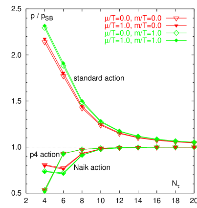
(a)

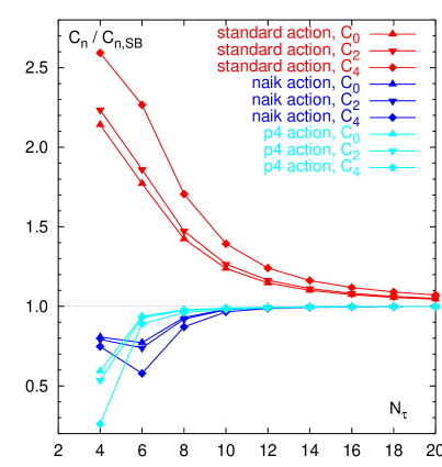
(b)

Figure 1: The pressure calculated on lattices with temporal extent $N_{\tau}$ in units of the continuum ideal Fermi gas value. (a) shows results for the standard, Naik and p4 actions at $(\mu_{q}/T,\,m/T)=(0,\,0),\,(0,\,1),(1,\,0)$ and $(1,\,1)$; (b) the coefficients ${\cal C}_{0},\,{\cal C}_{2},\,{\cal C}_{4}$ of the $\mu_{q}/T$ expansion of $p(m/T=0)$ divided by the corresponding SB constant as a function of $N_{\tau}$.

For the standard action cutoff effects remain $\geq 10$% out to $N_{\tau}\approx 16$, whereas both improved actions are hard to distinguish from the continuum result by $N_{\tau}=10$. We note that lines for different $\mu_{q}/T$ values but the same quark mass fall almost on top of each other. Cutoff effects are thus almost independent of $\mu_{q}$. The effect of $\mu_{q}\not=0$ on the cutoff dependence of the pressure is even smaller than the effect of quark mass $m\not=0$.

As can be seen from (32) for moderate values of $\mu_{q}/T$ the $\mu$-dependence of the continuum ideal gas pressure is dominated by the leading $O((\mu_{q}/T)^{2})$ contribution. In order to control the cut-off dependence of the various expansion terms we have expanded the integrand of (35) up to order $O((\mu_{q}/T)^{6})$. For the standard action the series starts with

$$\ln\left(\omega^{2}(p)+\sin^{2}\left(p_{4}-\frac{i}{N_{\tau}}\frac{\mu_{q}}{T}\right)\right)\,=\,\ln D$$ (39)

$$- \frac{2i\cos p_{4}\sin p_{4}}{D\,N_{\tau}}\left(\frac{\mu_{q}}{T}\right)$$

$$- \frac{-1+4\,D\,\cos 2p_{4}+\cos 4p_{4}}{4\,D^{2}\,N_{\tau}^{2}}\left(\frac{\mu_{q}}{T}\right)^{2}$$

$$- \frac{i\,\left(-1+4\,D^{2}+6\,D\,\cos 2p_{4}+\cos 4p_{4}\right)\,\sin 2p_{4}}{6\,D^{3}\,N_{\tau}^{3}}\left(\frac{\mu_{q}}{T}\right)^{3}$$

$$+ O\left(\left(\frac{\mu_{q}}{T}\right)^{4}\right).$$

Here we use the shorthand notation $D=4\sum_{\mu=1}^{4}f_{\mu}^{2}(p)$. The remaining orders as well as the series for Naik and p4 actions are given in Appendix B. A common feature of these expansions is that the odd terms are pure imaginary and the integral and sum over $p_{4}$ of those terms vanish due to a factor $\sin(np_{4})$ which always appears. To be more precise, this factor always forms the pattern $\sin(np_{4})\cos(mp_{4})$ which can be shown to vanish, either after summation over the discrete set of $p_{4}$ values, or integration from $0$ to $2\pi$, for $n,\,m\in\mathbb{N}$. Performing the momentum integration and the summation over Matsubara modes we obtain the coefficients of the ${\mu_{q}/T}$ expansion of the pressure;

$$\frac{p}{T^{4}}\Big{|}_{N_{\tau}}=N_{\rm f}\sum_{i=0}^{\infty}{\cal C}_{i}\Big{|}_{N_{\tau}}\left(\frac{\mu_{q}}{T}\right)^{i}\quad.$$ (40)

We checked numerically that with increasing $N_{\tau}$ the coefficients ${\cal C}_{0}$, ${\cal C}_{2}$ and ${\cal C}_{4}$ do indeed converge to their corresponding SB values,

$$\lim_{N_{\tau}\to\infty}{\cal C}_{0}=\frac{7\pi^{2}}{60};\quad\lim_{N_{\tau}\to\infty}{\cal C}_{2}=\frac{1}{2};\quad\lim_{N_{\tau}\to\infty}{\cal C}_{4}=\frac{1}{4\pi^{2}}.$$ (41)

Fig. 1b shows ${\cal C}_{0}$, ${\cal C}_{2}$ and ${\cal C}_{4}$ for the standard, Naik and p4 actions with massless quarks, normalized to the corresponding SB value.

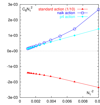
(a)

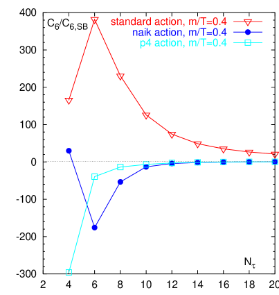
(b)

Figure 2: (a) The coefficients ${\cal C}_{6}$ in the massless case, multiplied with $N_{\tau}^{2}$ as a function of $N_{\tau}^{-2}$ (results for standard staggered fermions are divided by 10) and (b) the ratio ${\cal C}_{6}(N_{\tau})/{\cal C}_{6}(\infty)$ at $m/T=0.4$ for the standard, Naik and p4 actions.

We see here again that the cutoff dependence of the pressure at $\mu\not=0$ is qualitatively the same as at $\mu=0$.

For massless quarks the coefficient ${\cal C}_{6}$ should vanish with increasing $N_{\tau}$, as checked in Fig. 2a. It is expected that this term will approach zero like $N_{\tau}^{-2}$ in the large $N_{\tau}$ limit. In order to define the numerical factor, we plot ${\cal C}_{6}N_{\tau}^{2}$ over $N_{\tau}^{-2}$. A fit yields ${\cal C}_{6}\approx-0.015\,N_{\tau}^{-2}$ for the standard action. This is at least an order of magnitude larger than for the p4 improved action, for which the dominant cut-off dependence seems to be $O(N_{\tau}^{-4})$ as for the Naik action.

In the case of massive quarks the expansion (40) no longer terminates at ${\cal O}(\mu_{q}^{4})$. After expanding (31) in terms of $\mu_{q}/T$ and performing a numerical integration we find for the expansion coefficients ${\cal C}_{i}(m/T)$ up to $i=6$ the values given in Table 1.

	$m/T=0.4$		$m/T=1.0$
$i$	${\cal C}_{i}(m/T)$	${\cal C}_{i}(m/T)/{\cal C}_{i}(0)$	${\cal C}_{i}(m/T)$	${\cal C}_{i}(m/T)/{\cal C}_{i}(0)$
$0$	$1.113632$	0.967	$9.528163\cdot 10^{-1}$	0.827
$2$	$4.880455\cdot 10^{-1}$	0.976	$4.313914\cdot 10^{-1}$	0.863
$4$	$2.531101\cdot 10^{-2}$	0.999	$2.471397\cdot 10^{-2}$	0.976
$6$	$1.877659\cdot 10^{-6}$	—	$5.036816\cdot 10^{-5}$	—

Table 1: Continuum values for the coefficients ${\cal C}_{i}$ of the $\mu_{q}/T$ expansion of the pressure of a massive gas of quarks for the mass values $m/T=0.4$ and $m/T=1.0$.

The mass value $m/T=0.4$ is the value we use in our numerical calculations, corresponding to $N_{\tau}=4$ and $am=0.1$. We note that the coefficient ${\cal C}_{6}$ no longer vanishes. As shown in Fig. 2b, for $N_{\tau}$ finite there are large deviations from the continuum value. Even at $N_{\tau}=4$, however, the absolute value of this coefficient is still a factor of about $10^{-4}$ smaller than the leading term ${\cal C}_{0}$. The deviations thus do not show up in the calculation of the complete expression for the pressure shown in Figure 1a. These terms, however, become more important in higher derivatives of the pressure such as the quark number susceptibility $\chi_{q}$. In summary, for a gas of free quarks we find that the $\mu_{q}/T$ expansion up to $O((\mu_{q}/T)^{4})$ is sufficient for $\mu_{q}/T<1$ and $m/T<1$. In the continuum the deviation from the full expression over this range is smaller than 0.01%. On the lattice, however, cut-off effects lead to deviations of approximately 10% on coarse ($N_{\tau}=4$) lattices.

4 Numerical Results

We applied the formalism outlined in Sec. 2 to numerical simulations of QCD with $N_{\rm f}=2$ quark flavors on a $16^{3}\times 4$ lattice, using both Symanzik improved gauge and p4-improved staggered fermion actions. The simulation method is exactly as presented in [3] . The bare quark mass was $ma=0.1$ for which the pseudocritical point for zero chemical potential is estimated to be $\beta_{c}\simeq 3.649(2)$. In order to cover a range of temperatures on either side of the critical point we examined 16 values in the range $\beta\in[3.52,4.0]$. The simulation employed a hybrid molecular dynamic ‘R’-algorithm with discrete timestep $\delta\tau=0.025$, and measurements were performed on equilibrated configurations separated by $\tau=5$. In general for each $\beta$ 500 to 800 configurations were analysed, with 1000 used in the critical region $\beta\in[3.52,3.66]$. On each configuration 50 stochastic noise vectors were used to estimate the required fermionic operators. For each noise vector, 7 matrix inversions are required to estimate the required operators (8-11) and (49-52).

Following the procedure used for the equation of state at $\mu=0$ [15], we translate to physical units using the following scaling ansatz [18]:

$${{a(\beta)}\over{a(\bar{\beta})}}={\hat{a}}(\beta){{1+g_{2}\hat{a}^{2}(\beta)+g_{4}\hat{a}^{4}(\beta)}\over{1+g_{2}+g_{4}}}$$ (42)

where $\hat{a}\equiv R(\beta)/R(\bar{\beta})$, $R$ being the two-loop perturbative scaling function appropriate for two light flavors. Using string tension data at $(T,\mu)=(0,0)$ the best values for the fit parameters corresponding to a reference $\bar{\beta}=3.70$ are $g_{2}=0.669(208)$, $g_{4}=-0.0822(1088)$ [15]. We find that our simulations span a temperature range $T/T_{0}\in[0.76,1.98]$, where $T_{0}$ is the critical temperature at $\mu_{q}=0$.

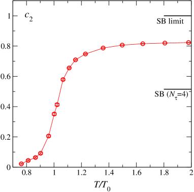
(a)

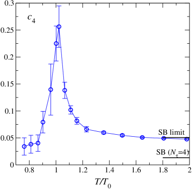
(b)

Figure 3: Coefficients of (a) $(\mu_{q}/T)^{2}$ and (b) $(\mu_{q}/T)^{4}$ in the Taylor expansion of $\Delta(p/T^{4})$ as functions of $T/T_{0}$.

In Fig. 3 we show the first two coefficients, (a) $c_{2}$ and (b) $c_{4}$, of the Taylor expansion of $\Delta(p/T^{4})$ introduced in (3) as functions of $T/T_{0}$. Also shown are the corresponding SB limits: (a) $N_{\rm f}{\cal C}_{2}(N_{\tau})$ and (b) $N_{\rm f}{\cal C}_{4}(N_{\tau})$, where the coefficients ${\cal C}_{i}$ are defined in (40), with values relevant for both the lattice used ($N_{\tau}=4$) and the continuum limit ($N_{\tau}=\infty$) plotted. Both $c_{2}$ and $c_{4}$ vary sharply in the critical region, but except in the immediate vicinity of the transition the quadratic term dominates the quartic. This is consistent with the results of [7] where data at varying $\mu$ obtained by reweighting was found lie on an almost universal curve when plotted as a fraction of the SB prediction. The asymptotic value of $c_{4}$ appears to be approached from above.

A notable feature is that in the high-$T$ limit our data lies closer to the continuum SB prediction rather than their values ${\cal C}_{i}(N_{\tau}=4)$ corrected for lattice artifacts, $c_{2}$ assuming 80% of the continuum value for $T/T_{0}=2$ whereas $c_{4}$ is almost coincident with its continuum value. By contrast recent calculations with unimproved staggered fermions [7, 9] find that the high-$T$ limit of the data lie close to the lattice-corrected SB value. This situation can be modelled by making the coefficient $d$ of the $O(N_{\tau}^{-2})$ correction appearing in (34) temperature dependent. In thermodynamic calculations performed with pure unimproved SU(3) lattice gauge theory [19], where extrapolations to the continuum limit are currently practicable, it is found that $d(T)\simeq 0.5d(T=\infty)$ for $T\sim 3T_{0}$, becoming even smaller closer to $T_{0}$. The behaviour of $c_{2}$ and $c_{4}$ we have observed using p4 fermions is broadly consistent with this behaviour.

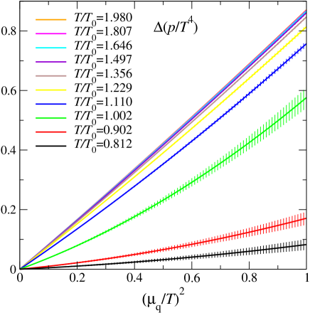
Figure 4: $\Delta(p/T^{4})$ as a function of $(\mu_{q}/T)^{2}$ for various temperatures, increasing upwards from the lowest curve with $T/T_{0}=0.812$ to the highest with $T/T_{0}=1.980$.

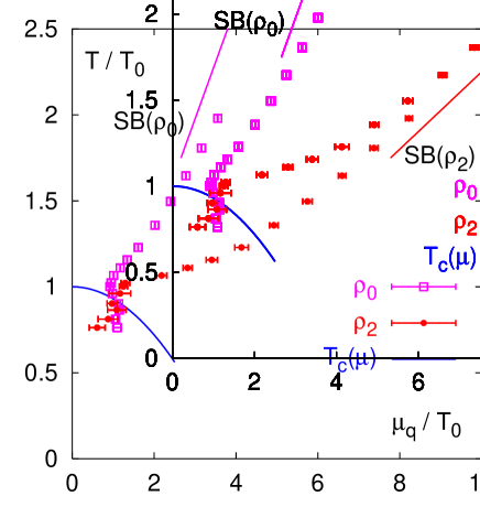
Figure 5: Estimates for the radius of convergence $\rho(\mu_{q},T)$.

In Fig. 4 we plot $\Delta(p/T^{4})$ defined in (3) as a function of $(\mu_{q}/T)^{2}$ for various temperatures. In most cases $c_{4}\ll c_{2}$ and the relation thus almost linear. The strongest departures from linearity are for $T\simeq T_{0}$, but even here the quadratic term is dominant for $(\mu_{q}/T)^{2}\raise 1.29167pt\hbox{$<$\kern-7.5pt\raise-4.73611pt\hbox{$\sim$}}0.4$, corresponding to $\mu_{q}\raise 1.29167pt\hbox{$<$\kern-7.5pt\raise-4.73611pt\hbox{$\sim$}}100$MeV. Given enough terms of the Taylor expansion in $\mu_{q}/T$, one could determine its radius of convergence $\rho$ via

$$\rho=\lim_{n\to\infty}\rho_{n}\equiv\lim_{n\to\infty}\sqrt{\left|{c_{n}\over c_{n+2}}\right|}.$$ (43)

Data from the pressure at $\mu_{q}=0$ [15] and the current study enable us to plot the first two estimates $\rho_{0}$ and $\rho_{2}$ on the $(\mu_{q},T)$ plane along with the estimated pseudocritical line $T_{c}(\mu_{q})$ found in [3] in Fig. 5. Also shown are the corresponding values from the SB limit (32). For $T>T_{c}$ one finds that $\rho_{n}$ increases markedly as $n$ increases from 0 to 2; if the SB limit is a good predictor for the QGP phase we might expect $c_{6}$ to be very small, and the next estimate $\rho_{4}$ correspondingly very large in this regime. Close to the transition line, however, the thermodynamic singularities appear to restrict $\rho\sim O(1)$; this in turn gives an approximate lower bound for the position of the critical endpoint. From the figure we deduce $\mu_{q}^{crit}\raise 1.29167pt\hbox{$>$\kern-7.5pt\raise-4.73611pt\hbox{$\sim$}}(1-1.2)T_{0}$, not inconsistent with the result of [2]. The new results at $O(\mu^{4})$ are important because they justify in retrospect our neglect of fourth order reweighting factors in our earlier calculation of the critical line $T_{c}(\mu_{q})$ [3]. Indeed, simulations with imaginary $\mu$ suggest that neglect of these terms in the analytic continuation to physical $\mu_{q}$ is justified for $\mu_{q}\raise 1.29167pt\hbox{$<$\kern-7.5pt\raise-4.73611pt\hbox{$\sim$}}170$MeV [4].

Fig. 7 plots the dimensionless correction $\Delta(p/T^{4})$ to the equation of state as a function of both $\mu_{q}/T$ and $\mu_{q}$. In the latter case the correction rises steeply across the transition and peaks for $T\simeq 1.1T_{0}$, before rapidly approaching a form $\Delta(p/T^{4})=\alpha T^{-2}$ characteristic of the SB limit, with the coefficient $\alpha$ having 82% of the continuum SB value. Comparison with the equation of state results at $\mu_{q}=0$ from Ref. [15] suggest that the correction will give a significant correction to the pressure for $0.9\raise 1.29167pt\hbox{$<$\kern-7.5pt\raise-4.73611pt\hbox{$\sim$}}T/T_{0}\raise 1.29167pt\hbox{$<$\kern-7.5pt\raise-4.73611pt\hbox{$\sim$}}1.3$, $\mu_{q}/T_{0}\raise 1.29167pt\hbox{$>$\kern-7.5pt\raise-4.73611pt\hbox{$\sim$}}0.5$, but will decrease in importance as $T$ rises further. The curves of Fig. 7b are in good qualitative agreement with those of Refs. [7, 9], although we consider any quantitative agreement to be somewhat accidental as the numerical data obtained in [7, 9] with unimproved actions have large discretisation errors which have been corrected for by renormalising the raw data with the known discretisation errors in the infinite temperature limit. Experience gained in calculations of thermodynamic quantities in the pure SU(3) gauge theory suggests that in the temperature range of a few times $T_{0}$ this procedure overestimates the importance of cut-off effects by a factor two or so [19].

Fig. 7a shows the quark number density $n_{q}$ evaluated using Eqn. (13). As $\mu_{q}$ increases, $n_{q}$ rises steeply as the QGP phase is entered; for reference, if the quark number density in nuclear matter is denoted $\bar{n}_{q}$, then the ratio $\bar{n}_{q}/T_{0}^{3}\approx 0.75$. Our results are numerically very similar to those obtained using exact reweighting in [7], where a mass $ma\approx 0.1$ for the light quark flavors was used. Note that a significant quark mass dependence for $n_{q}$ was observed in [3], and indeed is present even in the SB limit as described in Section 3; however analysis of the SB limit suggests that the difference between the chiral limit and $m/T=0.4$ is about 4%. In Fig. 7b we show the result of eliminating $\mu_{q}$ in favour of $n_{q}$ via

$$\Delta\left({p\over T^{4}}\right)={1\over{4c_{2}}}\left({n_{q}\over T^{3}}\right)^{2}-{3c_{4}\over 16c_{2}^{4}}\left({n_{q}\over T^{3}}\right)^{4}+O\biggl{(}\left({n_{q}\over T^{3}}\right)^{6}\biggr{)}.$$ (44)

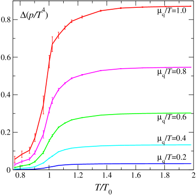
(a)

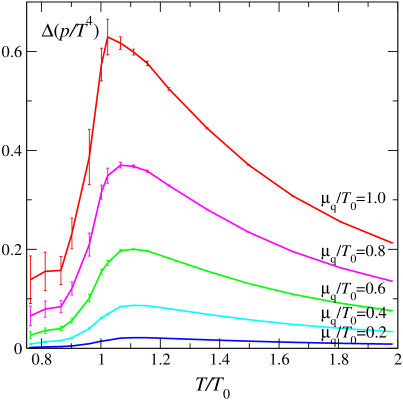
(b)

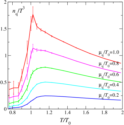
Figure 6: The equation of state correction $\Delta(p/T^{4})$ vs. $T/T_{0}$ for (a) various $\mu_{q}/T$, and (b) various $\mu_{q}/T_{0}$.

(a)

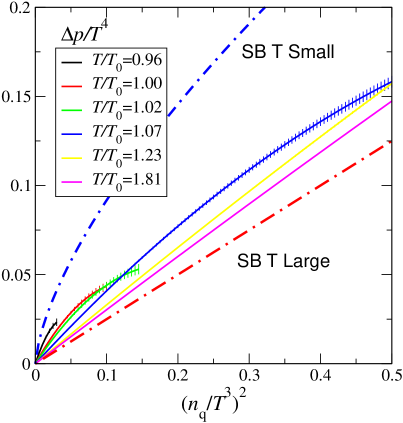
(b)

Figure 7: (a) $n_{q}/T^{3}$ as a function of $T/T_{0}$ for various $\mu_{q}/T_{0}$, and (b) the ”true” equation of state $\Delta(p/T^{4})$ vs. $(n_{q}/T^{3})^{2}$ for various temperatures. The continuum SB forms ${1\over 4}(\pi^{2}/N_{\rm f})^{1/3}(n_{q}/T^{3})^{4/3}$ (low $T$) and $(2N_{\rm f})^{-1}(n_{q}/T^{3})^{2}$ (high $T$) are also shown as functions of $T/T_{0}$.

The relation (44) approximates the “true” equation of state in terms of physically measurable quantities; we have plotted the resulting $\Delta(p/T^{4})$ against $(n_{q}/T^{3})^{2}$ up to the point where the ratio of the magnitude of the second term of (44) to that of the first is 40%: the point $n_{q}/T^{3}=\sqrt{2c_{2}^{3}/3c_{4}}$ where the ratio is 50% marks a mechanical instability $\partial p/\partial n_{q}=0$, which is an artifact due to the truncation of the series. Stability of the equilibrium state under local fluctuations $\delta n_{q}$ requires $\partial p/\partial n_{q}>0$, an example of Le Châtelier’s principle. As $T/T_{0}$ increases through unity, the equation of state changes from a form resembling the low-$T$ SB limit $p\propto n_{q}^{4/3}$ to the stiffer $p\propto n_{q}^{2}$ characteristic of the high-$T$ SB limit. Interestingly enough, to the order we have calculated the instability artifact sets in at $\mu_{q}/T\simeq 1.4$ for $T$ large, but at $\mu_{q}/T\simeq 0.4$ for $T\approx T_{0}$, thus providing an independent, and more stringent, limit to the physical validity of our approach, and reflecting the importance of contributions from higher orders in the Taylor expansion close to $T_{c}(\mu_{q})$.

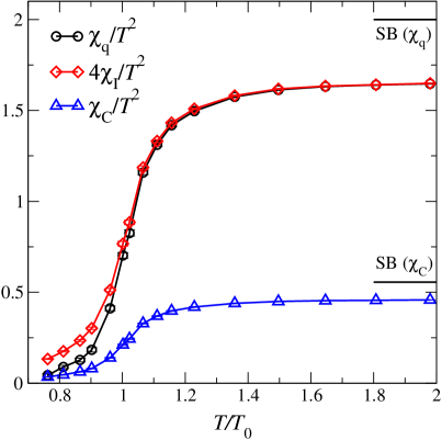
(a)

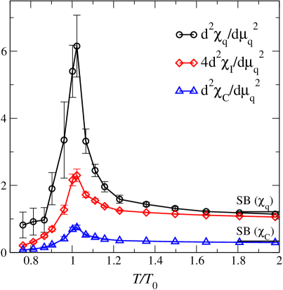
(b)

Figure 8: Susceptibilities (a) $\chi_{i}/T^{2}|_{\mu_{q}=0}$, and (b) $\partial^{2}\chi_{i}/\partial\mu_{q}^{2}|_{\mu_{q}=0}$ as functions of $T/T_{0}$.

Next, in Fig. 8 we plot the expansion coefficients corresponding to the various susceptibilities defined in (14-16). For $T\raise 1.29167pt\hbox{$<$\kern-7.5pt\raise-4.73611pt\hbox{$\sim$}}T_{0}$ there is a significant difference between $\chi_{q}(\mu_{q}=0)$ and $4\chi_{\rm I}(\mu_{q}=0)$, implying anti-correlated fluctuations of $n_{\rm u}$ and $n_{\rm d}$ which rapidly decrease in magnitude above $T_{0}$ and vanish as $T$ approaches the infinite temperature SB limit. In the same limit the charge susceptibility $\chi_{\rm C}$ approaches the value ${5\over 18}\chi_{q}$. The critical singularity in $4\chi_{\rm I}$ and $\chi_{\rm C}$ is weaker than that of $\chi_{q}$, which can be traced back to the differing coefficients of $\langle(\partial^{2}\ln\mbox{det}M/\partial\mu^{2})^{2}\rangle$, the dominant term in the vicinity of $T_{c}$, in the definitions (7) and (19). The dimensionless quantity $T\chi_{\rm C}/s$, where $s=(\epsilon+p-\mu_{q}n_{q})/T$ is the entropy density, can be related to event-by-event fluctuations in charged particle multiplicities in RHIC collisions, and has been proposed as a signal for QGP formation [25]. Event-by-event fluctuations in baryon number have also recently been discussed in [26].

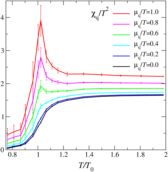
Figure 9: $\chi_{q}/T^{2}$ as a function of $T/T_{0}$ for various $\mu_{q}/T$.

In Fig. 9 the relation (17) and data of Fig. 3 have been used to plot the dimensionless quark number susceptibility $\chi_{q}/T^{2}$ as a function of $T/T_{0}$ for various $\mu_{q}/T$. The peak which develops in $\chi_{q}$ as $\mu_{q}$ increases is a sign that fluctuations in the baryon density are growing as the critical endpoint in the $(\mu,T)$ plane is approached. Physically, this shows that at the critical point, as well as strong fluctuations in the $(\bar{\psi}\psi)$ bilinear expected at a chiral phase transition there are also fluctuations in $(\bar{\psi}\gamma_{0}\psi)$ since Lorentz symmetry is explicitly broken by the background baryon charge density. For quantities such as $n_{q}$ and $\chi_{q}$ defined as higher derivatives of the free energy with respect to $\mu_{q}$, the relative importance of the higher order terms in the Taylor series expansion is increased; for example, at $T\simeq T_{0}$ and $\mu_{q}/T=1$ the quadratic contribution to $\chi_{q}(\mu_{q})$ is about 3 times that of the leading order term. For this reason we do not expect the data of Fig. 9 to be quantitatively accurate in the critical region. Note, however, that at each temperature the expansions for $p$, $n_{q}$ and $\chi_{q}$ all have the same radius of convergence.

(a)

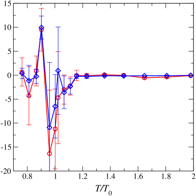
(b)

Figure 10: Derivatives (a) $(2VT^{3})^{-1}\partial^{3}\ln{\cal Z}/\partial\beta\partial(\mu_{q}/T)^{2}$ (circles) and $-(2VT^{3})^{-1}\partial^{3}\ln{\cal Z}/\partial m\partial(\mu_{q}/T)^{2}$ (diamonds); (b) $(24VT^{3})^{-1}\partial^{5}\ln{\cal Z}/\partial\beta\partial(\mu_{q}/T)^{4}$ (circles) and $-(24VT^{3})^{-1}\partial^{5}\ln{\cal Z}/\partial m\partial(\mu_{q}/T)^{4}$ (diamonds).

Finally we turn to a discussion of the derivatives necessary for calculating the response of the energy density $\epsilon$ to increasing $\mu_{q}$. The Taylor expansion of the energy density involves derivatives of the expansion coefficients $c_{p}(T)$ used to calculate the pressure,

$$\Delta\left({{\epsilon-3p}\over T^{4}}\right)=\sum_{p=1}^{\infty}c_{p}^{\prime}(T)\biggl{(}{\mu_{q}\over T}\biggr{)}^{p}\quad,$$ (45)

with $c_{p}^{\prime}(T)=T({\rm d}c_{p}(T)/{\rm d}T)|_{\mu_{q}=0}$. It is apparent from the temperature dependence of the expansion coefficients $c_{2}(T)$ and $c_{4}(T)$ shown in Fig. 3 that the coefficients $c_{p}^{\prime}(T)$ can become large in the vicinity of $T_{0}$. On the other hand that figure also shows that $c_{p}^{\prime}(T)$ will be small, i.e. close to zero, at high temperature as expected in the ideal gas limit. A comparison with (27) shows that the numerical evaluation of $c_{p}^{\prime}(T)$ requires the knowledge of lattice beta-functions and a calculation of mixed derivatives of $\ln{\cal Z}$ with respect to $\mu$ as well as $\beta$ and $m$. In Fig. 10 we plot these derivative terms; the signals in this case are much noisier than for $\partial^{n}\ln{\cal Z}/\partial\mu^{n}$, although we have been able to check that the numerical values for $\partial^{3}\ln{\cal Z}/\partial\beta\partial\mu^{2}$ are consistent with the slope of the curve in Fig. 3a. It is clear firstly that with the exception of $\partial^{3}\ln{\cal Z}/\partial m\partial\mu^{2}$ the signal only differs significantly from zero in the immediate neighbourhood of the transition, and secondly that derivatives with respect to $m$ are strongly anti-correlated with those with respect to $\beta$. The latter suggests it might be possible to learn something from (27) about the shape of the $\Delta((\epsilon-3p)/T^{4})$ curve as a function of $T/T_{0}$ away from the chiral limit even in the absence of quantitative information about $a\partial m/\partial a$.

Consider however ignoring mass derivatives and focusing on those performed with respect to coupling. In this case all derivatives are consistent with zero for $T\raise 1.29167pt\hbox{$>$\kern-7.5pt\raise-4.73611pt\hbox{$\sim$}}1.2\;T_{0}$; i.e. the difference $\Delta\left({{(\epsilon-3p)}/T^{4}}\right)$ is to a good approximation independent of $\mu_{q}$ for these high temperatures. This observation is consistent with the results obtained by using exact reweighting in [7]. Consider now temperatures close to $T_{0}$. The beta function at the critical $\beta_{c}$ has the value $a^{-1}da/d\beta=-2.08(43)$ [15]; substituting the derivatives from Fig. 10 in (27) we find at $T_{0}$

$$\Delta\left({{\epsilon-3p}\over T^{4}}\right)\approx(4.8\pm 1.2)\times\left({\mu_{q}\over T}\right)^{2}-(5\pm 4)\times\left({\mu_{q}\over T}\right)^{4}+\cdots$$ (46)

Taking the central values of the coefficients in this expansion one may conclude that the ratio $c_{2}^{\prime}/c_{4}^{\prime}$ is comparable with $c_{2}/c_{4}$. At present the large error on the coefficient of the $(\mu_{q}/T)^{4}$ term, however, does not allow a firm conclusion on the convergence radius of the expansion of $\epsilon-3p$. We also note that the coefficient $c_{4}^{\prime}$ will change sign for $T\sim T_{0}$. This suggests that large cancellations can occur for $\mu_{q}/T\sim{\cal O}(1)$ and indicates that higher order terms are needed to determine this difference reliably. In any event, it would appear that extending our current analysis to determine energy and entropy densities ($\epsilon$, $s$) in the critical region will be far more demanding.

5 Summary

We have presented the first Monte Carlo calculation of the QCD equation of state at non-zero quark chemical potential within the analytic framework; no reweighting has been performed. As in our previous work, we have exploited the relative simplicity of the method to explore larger physical volumes than those used in comparable studies [7, 9]. In addition, the compatibility of our method with the use of an improved lattice fermion action has meant that our results suffer from relatively mild discretisation artifacts, our data for the pressure correction $\Delta p(\mu_{q})$ achieving 80% of the Stefan-Boltzmann value by $T\simeq 2T_{0}$.

Our results for $\Delta p$ and its $\mu$-derivatives $n_{q}$ and the various susceptibilities $\chi_{i}$ are in good qualitative agreement with those of [7, 9]. Since higher derivatives suffer from larger discretisation artifacts, and are inherently noisier when estimated by Monte Carlo simulation, the results for, say, $\chi_{q}$ are less quantitatively reliable than those for $\Delta p$; nonetheless the singularity developing in $\chi_{q}$ as $\mu_{q}$ is increased, seen in Fig. 9, is evidence for the presence of a critical endpoint in the $(\mu_{q},T)$ plane, and for the importance of quark number fluctuations in its vicinity.

The calculation of fourth order derivatives has enabled us for the first time to make an estimate for the limitations of our method, both analytically through the radius of convergence of the Taylor expansion in $\mu_{q}/T$, and physically via the requirement of consistency with Le Châtelier’s principle. For both criteria the most stringent bounds are unsurprisingly in the vicinity of the critical line, where convergence of the series limits us to $\mu_{q}/T\raise 1.29167pt\hbox{$<$\kern-7.5pt\raise-4.73611pt\hbox{$\sim$}}1$, and mechanical stability of the equilibrium state to $\mu_{q}/T\raise 1.29167pt\hbox{$<$\kern-7.5pt\raise-4.73611pt\hbox{$\sim$}}0.5$. Of course, the picture should change with the inclusion of still higher derivatives since on physical grounds we expect stability of the equilibrium state everywhere within the domain of convergence. We are currently investigating the feasibility of including the relevant $O(\mu^{6})$ terms in our calculation.

Other quantities of phenomenological importance such as the energy $\epsilon$ and entropy $s$ densities, which require mixed derivatives with respect to the other bare parameters $\beta$ and $m$, appear more difficult to calculate with quantitative accuracy with this approach. It remains an open question whether the radius of convergence for these quantities is the same as that for quantities defined by series in $\partial^{n}\Omega/\partial\mu^{n}$.

Finally, it is necessary to stress the importance of refining the current calculation, firstly by simulating systems with $N_{\tau}\geq 6$ so that a reliable extrapolation to the continuum can be performed, and secondly by repeating it with a realistic spectrum of 2+1 fermion flavors.

Appendix A Derivatives needed to calculate energy density

Here we present the non-vanishing terms in the expressions for $\partial^{n+1}\ln{\cal Z}/\partial m\partial\mu^{n}$:

$$\frac{\partial^{3}\ln{\cal Z}}{\partial\mu^{2}\partial m}\hskip 34.14322pt=\left\langle\frac{N_{\rm f}}{4}\frac{\partial^{2}{\rm tr}M^{-1}}{\partial\mu^{2}}\right\rangle+2\left\langle\left(\frac{N_{\rm f}}{4}\right)^{2}\frac{\partial(\ln\det M)}{\partial\mu}\frac{\partial{\rm tr}M^{-1}}{\partial\mu}\right\rangle$$ (47)

$$+\left\langle\left(\frac{N_{\rm f}}{4}\right)^{2}\frac{\partial^{2}(\ln\det M)}{\partial\mu^{2}}{\rm tr}M^{-1}\right\rangle+\left\langle\left(\frac{N_{\rm f}}{4}\right)^{3}\left(\frac{\partial(\ln\det M)}{\partial\mu}\right)^{2}{\rm tr}M^{-1}\right\rangle$$

$$-\left[\left\langle\frac{N_{\rm f}}{4}\frac{\partial^{2}(\ln\det M)}{\partial\mu^{2}}\right\rangle+\left\langle\left(\frac{N_{\rm f}}{4}\frac{\partial(\ln\det M)}{\partial\mu}\right)^{2}\right\rangle\right]\left\langle\frac{N_{\rm f}}{4}{\rm tr}M^{-1}\right\rangle$$

$$\frac{\partial^{5}\ln{\cal Z}}{\partial\mu^{4}\partial m}\hskip 34.14322pt=\left\langle\frac{N_{\rm f}}{4}\frac{\partial^{4}({\rm tr}M^{-1})}{\partial\mu^{4}}\right\rangle+4\left\langle\left(\frac{N_{\rm f}}{4}\right)^{2}\frac{\partial^{3}({\rm tr}M^{-1})}{\partial\mu^{3}}\frac{\partial(\ln\det M)}{\partial\mu}\right\rangle$$ (48)

$$+4\left\langle\left(\frac{N_{\rm f}}{4}\right)^{2}\frac{\partial^{3}(\ln\det M)}{\partial\mu^{3}}\frac{\partial({\rm tr}M^{-1})}{\partial\mu}\right\rangle+6\left\langle\left(\frac{N_{\rm f}}{4}\right)^{2}\frac{\partial^{2}(\ln\det M)}{\partial\mu^{2}}\frac{\partial^{2}({\rm tr}M^{-1})}{\partial\mu^{2}}\right\rangle$$

$$+6\left\langle\left(\frac{N_{\rm f}}{4}\right)^{3}\frac{\partial^{2}({\rm tr}M^{-1})}{\partial\mu^{2}}\left(\frac{\partial(\ln\det M)}{\partial\mu}\right)^{2}\right\rangle$$

$$+12\left\langle\left(\frac{N_{\rm f}}{4}\right)^{3}\frac{\partial^{2}(\ln\det M)}{\partial\mu^{2}}\frac{\partial(\ln\det M)}{\partial\mu}\frac{\partial({\rm tr}M^{-1})}{\partial\mu}\right\rangle$$

$$+4\left\langle\left(\frac{N_{\rm f}}{4}\right)^{4}\left(\frac{\partial(\ln\det M)}{\partial\mu}\right)^{3}\frac{\partial({\rm tr}M^{-1})}{\partial\mu}\right\rangle+\left\langle\left(\frac{N_{\rm f}}{4}\right)^{2}\frac{\partial^{4}(\ln\det M)}{\partial\mu^{4}}{\rm tr}M^{-1}\right\rangle$$

$$+4\left\langle\left(\frac{N_{\rm f}}{4}\right)^{3}\frac{\partial^{3}(\ln\det M)}{\partial\mu^{3}}\frac{\partial(\ln\det M)}{\partial\mu}{\rm tr}M^{-1}\right\rangle$$

$$+3\left\langle\left(\frac{N_{\rm f}}{4}\right)^{3}\left(\frac{\partial^{2}(\ln\det M)}{\partial\mu^{2}}\right)^{2}{\rm tr}M^{-1}\right\rangle$$

$$+6\left\langle\left(\frac{N_{\rm f}}{4}\right)^{4}\frac{\partial^{2}(\ln\det M)}{\partial\mu^{2}}\left(\frac{\partial(\ln\det M)}{\partial\mu}\right)^{2}{\rm tr}M^{-1}\right\rangle$$

$$+\left\langle\left(\frac{N_{\rm f}}{4}\right)^{5}\left(\frac{\partial(\ln\det M)}{\partial\mu}\right)^{4}{\rm tr}M^{-1}\right\rangle$$

$$-\Biggl{[}\left\langle\frac{N_{\rm f}}{4}\frac{\partial^{4}(\ln\det M)}{\partial\mu^{4}}\right\rangle+4\left\langle\left(\frac{N_{\rm f}}{4}\right)^{2}\frac{\partial^{3}(\ln\det M)}{\partial\mu^{3}}\frac{\partial(\ln\det M)}{\partial\mu}\right\rangle$$

$$+3\left\langle\left(\frac{N_{\rm f}}{4}\right)^{2}\left(\frac{\partial^{2}(\ln\det M)}{\partial\mu^{2}}\right)^{2}\right\rangle+\left\langle\left(\frac{N_{\rm f}}{4}\frac{\partial(\ln\det M)}{\partial\mu}\right)^{4}\right\rangle$$

$$+6\left\langle\left(\frac{N_{\rm f}}{4}\right)^{3}\frac{\partial^{2}(\ln\det M)}{\partial\mu^{2}}\left(\frac{\partial(\ln\det M)}{\partial\mu}\right)^{2}\right\rangle\Biggr{]}\left\langle\frac{N_{\rm f}}{4}{\rm tr}M^{-1}\right\rangle$$

$$-6\left[\left\langle\frac{N_{\rm f}}{4}\frac{\partial^{2}({\rm tr}M^{-1})}{\partial\mu^{2}}\right\rangle+2\left\langle\left(\frac{N_{\rm f}}{4}\right)^{2}\frac{\partial(\ln\det M)}{\partial\mu}\frac{\partial({\rm tr}M^{-1})}{\partial\mu}\right\rangle\right.$$

$$+\left\langle\left(\frac{N_{\rm f}}{4}\right)^{2}\frac{\partial^{2}(\ln\det M)}{\partial\mu^{2}}{\rm tr}M^{-1}\right\rangle+\left\langle\left(\frac{N_{\rm f}}{4}\right)^{3}\left(\frac{\partial(\ln\det M)}{\partial\mu}\right)^{2}{\rm tr}M^{-1}\right\rangle$$

$$\left.-\left(\left\langle\frac{N_{\rm f}}{4}\frac{\partial^{2}(\ln\det M)}{\partial\mu^{2}}\right\rangle+\left\langle\left(\frac{N_{\rm f}}{4}\frac{\partial(\ln\det M)}{\partial\mu}\right)^{2}\right\rangle\right)\left\langle\frac{N_{\rm f}}{4}{\rm tr}M^{-1}\right\rangle\right]$$

$$\times\left[\left\langle\frac{N_{\rm f}}{4}\frac{\partial^{2}(\ln\det M)}{\partial\mu^{2}}\right\rangle+\left\langle\left(\frac{N_{\rm f}}{4}\frac{\partial(\ln\det M)}{\partial\mu}\right)^{2}\right\rangle\right].$$

As explained above, all terms involving the expectation value of an odd number of derivations with respect to $\mu$ have been set to zero. Evaluation of eqns. (47) and (48) requires the following expressions for the derivatives of $\mbox{tr}M^{-1}$:

$$\frac{\partial{\rm tr}M^{-1}}{\partial\mu}=-{\rm tr}\left(M^{-1}\frac{\partial M}{\partial\mu}M^{-1}\right)$$ (49)

$$\frac{\partial^{2}{\rm tr}M^{-1}}{\partial\mu^{2}}=-{\rm tr}\left(M^{-1}\frac{\partial^{2}M}{\partial\mu^{2}}M^{-1}\right)+2{\rm tr}\left(M^{-1}\frac{\partial M}{\partial\mu}M^{-1}\frac{\partial M}{\partial\mu}M^{-1}\right)$$ (50)

$$\frac{\partial^{3}{\rm tr}M^{-1}}{\partial\mu^{3}}=-{\rm tr}\left(M^{-1}\frac{\partial^{3}M}{\partial\mu^{3}}M^{-1}\right)+3{\rm tr}\left(M^{-1}\frac{\partial^{2}M}{\partial\mu^{2}}M^{-1}\frac{\partial M}{\partial\mu}M^{-1}\right)$$ (51)

$$+3{\rm tr}\left(M^{-1}\frac{\partial M}{\partial\mu}M^{-1}\frac{\partial^{2}M}{\partial\mu^{2}}M^{-1}\right)-6{\rm tr}\left(M^{-1}\frac{\partial M}{\partial\mu}M^{-1}\frac{\partial M}{\partial\mu}M^{-1}\frac{\partial M}{\partial\mu}M^{-1}\right)$$

$$\frac{\partial^{4}{\rm tr}M^{-1}}{\partial\mu^{4}}=-{\rm tr}\left(M^{-1}\frac{\partial^{4}M}{\partial\mu^{4}}M^{-1}\right)+4{\rm tr}\left(M^{-1}\frac{\partial^{3}M}{\partial\mu^{3}}M^{-1}\frac{\partial M}{\partial\mu}M^{-1}\right)$$ (52)

$$+6{\rm tr}\left(M^{-1}\frac{\partial^{2}M}{\partial\mu^{2}}M^{-1}\frac{\partial^{2}M}{\partial\mu^{2}}M^{-1}\right)+4{\rm tr}\left(M^{-1}\frac{\partial M}{\partial\mu}M^{-1}\frac{\partial^{3}M}{\partial\mu^{3}}M^{-1}\right)$$

$$-12{\rm tr}\left(M^{-1}\frac{\partial^{2}M}{\partial\mu^{2}}M^{-1}\frac{\partial M}{\partial\mu}M^{-1}\frac{\partial M}{\partial\mu}M^{-1}\right)$$

$$-12{\rm tr}\left(M^{-1}\frac{\partial M}{\partial\mu}M^{-1}\frac{\partial^{2}M}{\partial\mu^{2}}M^{-1}\frac{\partial M}{\partial\mu}M^{-1}\right)$$

$$-12{\rm tr}\left(M^{-1}\frac{\partial M}{\partial\mu}M^{-1}\frac{\partial M}{\partial\mu}M^{-1}\frac{\partial^{2}M}{\partial\mu^{2}}M^{-1}\right)$$

$$+24{\rm tr}\left(M^{-1}\frac{\partial M}{\partial\mu}M^{-1}\frac{\partial M}{\partial\mu}M^{-1}\frac{\partial M}{\partial\mu}M^{-1}\frac{\partial M}{\partial\mu}M^{-1}\right)$$

Appendix B The pressure of free staggered fermions

Expanding the quantity $p/T^{4}$ as discussed in section 3 one finds

$$\frac{p}{T^{4}}\Big{|}_{N_{\tau}}=N_{\rm f}\sum_{i=0}^{\infty}\mathcal{C}_{i}\Big{|}_{N_{\tau}}\left(\frac{\mu}{T}\right)^{i}\;=\;\frac{3}{8}N_{\rm f}\Bigg{[}\sum_{i=0}^{\infty}\left(\frac{N_{\tau}^{3-i}}{(2\pi)^{3}}\int_{0}^{2\pi}d^{3}\vec{p}\,\sum_{p_{4}}\,c_{i}(p)\,\right)\left(\frac{\mu}{T}\right)^{i}$$ (53)

$$-\frac{N_{\tau}^{4}}{(2\pi)^{4}}\int_{0}^{2\pi}d^{4}p\,\,c_{0}(p)\,\Bigg{]}~{}~{}.$$

Here only the even expansion coefficients give non-vanishing contributions. Introducing the abbreviation,

$$D=4\sum_{\mu}f^{2}_{\mu}(p),$$ (54)

with $f_{\mu}(p)$ as given in (38), the even expansion coefficients for the standard action are given by:

$$c_{0} = \ln(D)$$ (55)

$$c_{2} = \frac{1}{4D^{2}}\big{(}1-4D\cos(2p_{4})-\cos(4p_{4})\big{)}$$ (56)

$$c_{4} = \frac{1}{96D^{4}}\big{(}-9+8D^{2}-8D(-3+4D^{2})\cos(2p_{4})$$ (57)

$$+(12-56D^{2})\cos(4p_{4})-24D\cos(6p_{4})-3\cos(8p_{4})\big{)}$$

$$c_{6} = \frac{1}{2880D^{6}}\big{(}150-180D^{2}+32D^{4}-8D(45-60D^{2}$$ (58)

$$+16D^{4})\cos(2p_{4})+(-225+960D^{2}-992D^{4})\cos(4p_{4})$$

$$+540D\cos(6p_{4})-1440D^{3}\cos(6p_{4})+90\cos(8p_{4})$$

$$-780D^{2}\cos(8p_{4})-180D\cos(10p_{4})-15\cos(12p_{4})\big{)},$$

For the Naik action we introduce an additional function,

$$g_{4}(p)\equiv\left.-i\frac{df_{4}(\vec{p},p_{4}-i\mu)}{d\mu}\right|_{\mu=0}=-\frac{9}{16}\cos(p_{4})+\frac{3}{48}\cos(3p_{4}),$$ (59)

The even expansion coefficients can then be written as:

$$c_{0} = \ln(D)$$ (60)

$$c_{2} = \frac{-2}{3D^{2}}\big{(}-6Df_{4}^{2}(p)+6Dg_{4}^{2}(p)-48f_{4}^{2}(p)g_{4}^{2}(p)$$ (61)

$$+Df_{4}(p)\sin(3p_{4})\big{)}$$

$$c_{4} = \frac{1}{36D^{4}}\Big{(}48\big{(}-768f_{4}^{4}(p)g_{4}^{4}(p)+D^{3}\big{(}f_{4}^{2}(p)-g_{4}^{2}(p)\big{)}$$ (62)

$$-192Df_{4}^{2}(p)g_{4}^{2}(p)\big{(}f_{4}^{2}(p)-g_{4}^{2}(p)\big{)}+D^{2}\big{(}-6f_{4}^{4}(p)$$

$$+44f_{4}^{2}(p)g_{4}^{2}(p)-6g_{4}^{4}(p)\big{)}\big{)}-24D^{2}\big{(}D-8f_{4}^{2}(p)\big{)}g_{4}(p)\cos(3p_{4})$$

$$-32D{f_{4}(p)}\big{(}D^{2}-3Df_{4}^{2}(p)+9Dg_{4}^{2}(p)-48f_{4}^{2}(p)g_{4}^{2}(p)\big{)}\sin(3p_{4})$$

$$+D^{2}\big{(}D-8f_{4}^{2}(p)\big{)}\sin^{2}(3p_{4})\Big{)}$$

$$c_{6} = \frac{1}{1620D^{6}}\Big{(}-720D^{2}g_{4}(p)\big{(}D^{3}+768f_{4}^{4}(p)g_{4}^{2}(p)+D^{2}\big{(}-26f_{4}^{2}(p)$$ (63)

$$+6g_{4}^{2}(p)\big{)}+96D\big{(}f_{4}^{4}(p)-2f_{4}^{2}(p)g_{4}^{2}(p)\big{)}\big{)}\cos(3p_{4})$$

$$-45D^{4}\big{(}D-8f_{4}^{2}(p)\big{)}\cos^{2}(3p_{4})-96Df_{4}(p)\big{(}8D^{4}+46080f_{4}^{4}(p)g_{4}^{4}(p)$$

$$-75D^{3}\big{(}f_{4}^{2}(p)-3g_{4}^{2}(p)\big{)}+60D^{2}\big{(}3f_{4}^{4}(p)-50f_{4}^{2}(p)g_{4}^{2}(p)+15g_{4}^{4}(p)\big{)}$$

$$+2880D\big{(}3f_{4}^{4}(p)g_{4}^{2}(p)-5f_{4}^{2}(p)g_{4}^{4}(p)\big{)}\big{)}\sin(3p_{4})+15D^{2}\big{(}5D^{3}$$

$$+4608f_{4}^{4}(p)g_{4}^{2}(p)+D^{2}\big{(}-76f_{4}^{2}(p)+36g_{4}^{2}(p)\big{)}+192D\big{(}f_{4}^{4}(p)$$

$$-6f_{4}^{2}(p)g_{4}^{2}(p)\big{)}\big{)}\sin^{2}(3p_{4})+10D^{3}f_{4}(p)\big{(}3D-16f_{4}^{2}(p)\big{)}\sin^{3}(3p_{4})$$

$$+72\big{(}4\big{(}245760{f_{4}(p)}^{6}g_{4}^{6}(p)+D^{5}\big{(}f_{4}^{2}(p)-g_{4}^{2}(p)\big{)}$$

$$+92160Df_{4}^{4}(p)g_{4}^{4}(p)\big{(}f_{4}^{2}(p)-g_{4}^{2}(p)\big{)}-2D^{4}\big{(}15f_{4}^{4}(p)-94f_{4}^{2}(p)g_{4}^{2}(p)$$

$$+15g_{4}^{4}(p)\big{)}+120D^{3}\big{(}f_{4}^{6}(p)-23f_{4}^{4}(p)g_{4}^{2}(p)+23f_{4}^{2}(p)g_{4}^{4}(p)-g_{4}^{6}(p)\big{)}$$

$$+960D^{2}\big{(}9f_{4}^{6}(p)g_{4}^{2}(p)-34f_{4}^{4}(p)g_{4}^{4}(p)+9f_{4}^{2}(p)g_{4}^{6}(p)\big{)}\big{)}$$

$$-5D^{3}f_{4}(p)\big{(}3D-16f_{4}^{2}(p)\big{)}g_{4}(p)\sin(6p_{4})\big{)}\Big{)}$$

To simplify the expressions for the p4 action we define the expansion coefficients recursively and thus also list the odd expansion coefficients. However, after integration over the momenta also in this case only even powers of $\mu/T$ contribute to the expansion of the pressure. Introducing further abbreviations,

$$S_{\mu}=\sum_{\nu\neq\mu}\sin^{2}(p_{\nu})\qquad\mbox{and}\qquad\bar{c}_{k}=-ic_{k},$$ (64)

the expansion coefficients for the p4 action can be written as

$$c_{0} = \ln(D)$$ (65)

$$c_{1} = -\frac{i}{6D}\big{(}-S_{1}-S_{2}-S_{3}+6S_{4}^{2}+S_{1}\cos(2p_{1})+S_{2}\cos(2p_{2})$$ (66)

$$+S_{3}\cos(2p_{3})\big{)}\sin(2p_{4})$$

$$c_{2} = \frac{1}{18D}\big{(}9D\bar{c}_{1}^{2}+6\big{(}3S^{2}_{4}-S_{1}\sin^{2}(p_{1})-S_{2}\sin^{2}(p_{2})$$ (67)

$$-S_{3}\sin^{2}(p_{3})\big{)}\sin^{2}(p_{4})-2\cos^{2}(p_{4})\big{(}9S^{2}_{4}$$

$$+\sin^{2}(p_{1})\big{(}-3S_{1}+\sin^{2}(p_{4})\big{)}+\sin^{2}(p_{2})\big{(}-3S_{2}+\sin^{2}(p_{4})\big{)}$$

$$+\sin^{2}(p_{3})\big{(}-3S_{3}+\sin^{2}(p_{4})\big{)}\big{)}\big{)}$$

$$c_{3} = \frac{i}{18D}\big{(}3D\bar{c}_{1}\big{(}\bar{c}_{1}^{2}-6c_{2}\big{)}-\big{(}-3+\cos(2p_{1})+\cos(2p_{2})$$ (68)

$$+\cos(2p_{3})\big{)}\cos^{3}(p_{4})\sin(p_{4})-2\cos(p_{4})\sin(p_{4})\big{(}12S_{4}^{2}$$

$$+\sin^{2}(p_{1})\big{(}-4S_{1}+\sin^{2}(p_{4})\big{)}+\sin^{2}(p_{2})\big{(}-4S_{2}+\sin^{2}(p_{4})\big{)}$$

$$+\sin^{2}(p_{3})\big{(}-4S_{3}+\sin^{2}(p_{4})\big{)}\big{)}\big{)}$$

$$c_{4} = \frac{1}{216D}\big{(}6\cos^{4}(p_{4})\big{(}\sin^{2}(p_{1})+\sin^{2}(p_{2})+\sin^{2}(p_{3})\big{)}$$ (69)

$$-3\big{(}3D\big{(}\bar{c}_{1}^{4}-12\bar{c}_{1}^{2}c_{2}+12c_{2}^{2}-24\bar{c}_{1}\bar{c}_{3}\big{)}+8\big{(}-3S_{4}^{2}+S_{1}\sin^{2}(p_{1})$$

$$+S_{2}\sin^{2}(p_{2})+S_{3}\sin^{2}(p_{3})\big{)}\sin^{2}(p_{4})+\big{(}-3+\cos(2p_{1})$$

$$+\cos(2p_{2})+\cos(2p_{3})\big{)}\sin^{4}(p_{4}))-4\cos^{2}(p_{4})\big{(}18S_{4}^{2}$$

$$+\sin^{2}(p_{1})\big{(}-6S_{1}+11\sin^{2}(p_{1})\big{)}+\sin^{2}(p_{2})\big{(}-6S_{2}+11\sin^{2}(p_{2})\big{)}$$

$$+\sin^{2}(p_{3})\big{(}-6S_{3}+11\sin^{2}(p_{3})\big{)}\big{)}\big{)}$$

$$c_{5} = -\frac{i}{360D}\big{(}3D\big{(}\bar{c}_{1}^{5}-20c_{1}^{3}c_{2}-60\bar{c}_{1}^{2}\bar{c}_{3}+120{c}_{2}\bar{c}_{3}+60\bar{c}_{1}\big{(}c_{2}^{2}+2c_{4}\big{)}\big{)}$$ (70)

$$+20\big{(}-3+\cos(2p_{1})+\cos(2p_{2})+\cos(2p_{3})\big{)}\cos^{3}(p_{4})\sin(p_{4})$$

$$+8\cos(p_{4})\sin(p_{4})\big{(}12S_{4}^{2}+\sin^{2}(p_{1})\big{(}-4S_{1}+5\sin^{2}(p_{4})\big{)}$$

$$+\sin^{2}(p_{2})\big{(}-4S_{2}+5\sin^{2}(p_{4})\big{)}+\sin^{2}(p_{3})\big{(}-4S_{3}+5\sin^{2}(p_{4})\big{)}\big{)}\big{)}$$

$$c_{6} = -\frac{1}{6480D}\big{(}6-9D\bar{c}_{1}^{6}+270D\bar{c}_{1}^{4}c_{2}-1620D\bar{c}_{1}^{2}c_{2}^{2}+1080Dc_{2}^{3}$$ (71)

$$+1080D\bar{c}_{1}^{3}\bar{c}_{3}-6480D\bar{c}_{1}c_{2}\bar{c}_{3}-3240D\bar{c}_{3}^{2}-3240D\bar{c}_{1}^{2}c_{4}$$

$$+6480Dc_{2}c_{4}-6480D\bar{c}_{1}\bar{c}_{5}-2\cos(2p_{1})-2\cos(2p_{2})-2\cos(2p_{3})$$

$$+31\cos(2(p_{1}-2p_{4}))+31\cos(2(p_{2}-2p_{4}))+31\cos(2(p_{3}-2p_{4}))$$

$$+24S_{1}\cos(2(p_{1}-p_{4}))+24S_{2}\cos(2(p_{2}-p_{4}))+24S_{3}\cos(2(p_{3}-p_{4}))$$

$$-48S_{1}\cos(2p_{4})-48S_{2}\cos(2p_{4})-48S_{3}\cos(2p_{4})+288S_{4}^{2}\cos(2p_{4})$$

$$-186\cos(4p_{4})+24S_{1}\cos(2(p_{1}+p_{4}))+24S_{2}\cos(2(p_{2}+p_{4}))$$

$$+24S_{3}\cos(2(p_{3}+p_{4}))+31\cos(2(p_{1}+2p_{4}))$$

$$+31\cos(2(p_{2}+2p_{4}))+31\cos(2(p_{3}+2p_{4}))\big{)}.$$

Note that we have defined here the coefficients $c_{i}$ without $N_{\tau}$ factors, which can be found in front of the integrals in (53).

References

- [1] S. Choe et al. [QCDTARO collaboration], Phys. Rev. D65 (2002) 054501.
- [2] Z. Fodor and S. Katz, JHEP 0203 (2002) 014.
- [3] C.R. Allton, S. Ejiri, S.J. Hands, O. Kaczmarek, F. Karsch, E. Laermann, Ch. Schmidt and L. Scorzato, Phys. Rev. D66 (2002) 074507.
- [4] P. de Forcrand and O. Philipsen, Nucl. Phys. B642 (2002) 290.
- [5] P. Braun-Munzinger, D. Magestro, K. Redlich and J. Stachel, Phys. Lett. B518 (2001) 41.
- [6] Z. Fodor and S.D. Katz, Phys. Lett. B534 (2002) 87.
- [7] Z. Fodor, S.D. Katz and K.K. Szabó, hep-lat/0208078.
- [8] S. Gottlieb, W. Liu, D. Toussaint, R.L. Renken and R.L. Sugar, Phys. Rev. D38 (1988) 2888.
- [9] R.V. Gavai and S. Gupta, hep-lat/0303013.
- [10] M. D’Elia and M.-P. Lombardo, Phys. Rev. D67 (2003) 014505.
- [11] A. Hart, M. Laine and O. Philipsen, Phys. Lett. B505 (2001) 141.
- [12] Ch. Schmidt, C.R. Allton, S. Ejiri, S.J. Hands, O. Kaczmarek, F. Karsch and E. Laermann, Nucl. Phys. B (Proc. Suppl.) 119 (2003) 517.
- [13] S. Naik, Nucl. Phys. B316 (1989) 238.
- [14] U.M. Heller, F. Karsch and B. Sturm, Phys. Rev. D60 (1999) 114502.
- [15] F. Karsch, E. Laermann and A. Peikert, Phys. Lett. B478 (2000) 447.
- [16] A. Ali Khan et al. [CP-PACS collaboration], Phys. Rev. D64 (2001) 074510.
- [17] Y. Liu, H. Matsufuru, O. Miyamura, A. Nakamura and T. Takaishi, Soryushiron Kenkyu (Kyoto) 105 (2002) D77.
- [18] C.R. Allton, hep-lat/9610016 and Nucl. Phys. B (Proc. Suppl.) 53 (1997) 867.
- [19] G. Boyd, J. Engels, F. Karsch, E. Laermann, C. Legeland, M. Lutgemeier and B. Petersson, Nucl. Phys. B469 (1996) 419.
- [20] A. Roberge and N. Weiss, Nucl. Phys. B275 (1986) 734.
- [21] R.V. Gavai and S. Gupta, Phys. Rev. D65 (2002) 094515.
- [22] J.-P. Blaizot, E. Iancu and A. Rebhan, Phys. Lett. B523 (2001) 143.
- [23] J.-P. Blaizot, E. Iancu and A. Rebhan, Eur. Phys. J. C 27 (2003) 433.
- [24] C. Bernard et al. [MILC Collaboration], hep-lat/0209079.
-
[25]
M. Asakawa, U. Heinz and B. Müller,
Phys. Rev. Lett. 85 (2000) 2072;
S. Jeon and V. Koch, Phys. Rev. Lett. 85 (2000) 2076; hep-ph/0304012. - [26] Y. Hatta and M.A. Stephanov, hep-ph/0302002.