DESY 02-149
Edinburgh 2002/11
LU-ITP 2002/019
September 2002
Calculation of Moments of Structure Functions

Abstract

The progress on the lattice computation of low moments of both the unpolarised and polarised nucleon structure functions is reviewed with particular emphasis on continuum and chiral extrapolations and comparison between quenched and unquenched fermions.

1 INTRODUCTION

Deep Inelastic Scattering (DIS) experiments, such as $eN\to eX$ or $\nu N\to\mu^{-}X$ form an important basis for our knowledge of the structure of hadrons. In these processes the current probe (either a neutral current, $\gamma$/$Z^{0}$, or charged current, $W^{+}$/$W^{-}$) with large space-like momentum $-q^{2}\equiv Q^{2}$ breaks-up the nucleon. The (inclusive) cross section is then determined by the structure functions $F_{1}$, $F_{2}$ when summing over beam and target polarisations and, in addition, $F_{3}$ when using neutrino beams, and $g_{1}$, $g_{2}$ when both the beam and target are suitably polarised. The structure functions are functions of the Bjorken variable $x$ ($0\leq x\leq 1$) and $Q^{2}$. (Another class of structure functions – the transversity $h_{1}$ – can be measured, in principle, from Drell-Yan type processes or in certain semi-inclusive processes [2].) While the original pioneering discoveries were made over thirty years ago at SLAC, more recently experiments with polarised beams have been reported and the field remains very active. Recent experiments and proposals, [3, 4], include H1 and Zeus at DESY (unpolarised $F_{2}$ at small $x$, [5] and $F_{3}$, [6]), Hermes at DESY (polarised $g_{1}$ and $g_{2}$, [7]), E155 at SLAC (polarised $g_{1}$, $g_{2}$, [8]), Jefferson lab (structure functions in the resonance region, [9, 10]), COMPASS at CERN (polarised gluon distribution, $h_{1}$, $\Lambda$ matrix elements, [11]), CCFR at Fermilab (unpolarised $F_{3}$, [12]) and RHIC (spin physics, [13]). Recent results are given in the DIS conference series, [14].

A direct theoretical calculation of the structure functions seems not to be possible (but see [15, 16, 17]); however using the Wilson Operator Product Expansion (OPE) we may relate moments of the structure functions to matrix elements of certain operators in a twist or Taylor expansion in $1/Q^{2}$. Thus if we define

$${\cal O}^{\gamma;\mu_{1}\cdots\mu_{n}} = \bar{q}\gamma^{\mu_{1}}i\mbox{ \parbox[b]{0.0pt}{$D$}\raisebox{7.3194pt}{$\leftrightarrow$}${}_{\!}$}^{\mu_{2}}\cdots i\mbox{ \parbox[b]{0.0pt}{$D$}\raisebox{7.3194pt}{$\leftrightarrow$}${}_{\!}$}^{\mu_{n}}q$$

$${\cal O}^{\gamma\gamma_{5};\sigma\mu_{1}\ldots\mu_{n}} = \bar{q}\gamma^{\sigma}\gamma_{5}i\mbox{ \parbox[b]{0.0pt}{$D$}\raisebox{7.3194pt}{$\leftrightarrow$}${}_{\!}$}^{\mu_{1}}\cdots i\mbox{ \parbox[b]{0.0pt}{$D$}\raisebox{7.3194pt}{$\leftrightarrow$}${}_{\!}$}^{\mu_{n}}q$$

$${\cal O}^{\sigma\gamma_{5};\sigma\mu_{1}\ldots\mu_{n}} = \bar{q}\sigma^{\sigma\mu_{1}}\gamma_{5}i\mbox{ \parbox[b]{0.0pt}{$D$}\raisebox{7.3194pt}{$\leftrightarrow$}${}_{\!}$}^{\mu_{2}}\cdots i\mbox{ \parbox[b]{0.0pt}{$D$}\raisebox{7.3194pt}{$\leftrightarrow$}${}_{\!}$}^{\mu_{n}}q$$

then we have the Lorentz decompositions

$$\langle N(\vec{p})|{\cal O}^{\gamma;\{\mu_{1}\cdots\mu_{n}\}}-\mbox{tr}|N(\vec{p})\rangle=$$

$$2v_{n}\,\left[p^{\mu_{1}}\cdots p^{\mu_{n}}-\mbox{tr}\right]$$

$$\langle N(\vec{p},\vec{s})|{\cal O}^{\gamma\gamma_{5};\{\sigma\mu_{1}\cdots\mu_{n}\}}-\mbox{tr}|N(\vec{p},\vec{s})\rangle=$$

$$2{a_{n}\over n+1}\,\left[s^{\sigma}p^{\mu_{1}}\cdots p^{\mu_{n}}-\mbox{tr}\right]$$

$$\langle N(\vec{p},\vec{s})|{\cal O}^{\gamma\gamma_{5};[\sigma\{\mu_{1}]\cdots\mu_{n}\}}-\mbox{\rm tr}|N(\vec{p},\vec{s})\rangle=$$

$${n\over{n+1}}d_{n}\,\left[(s^{\sigma}p^{\{\mu_{1}}-s^{\{\mu_{1}}p^{|\sigma|})p^{\mu_{2}}\cdots p^{\mu_{n}\}}-\mbox{\rm tr}\right]$$

$$\langle N(\vec{p},\vec{s})|{\cal O}^{\sigma\gamma_{5};\sigma\{\mu_{1}\cdots\mu_{n}\}}-\mbox{tr}|N(\vec{p},\vec{s})\rangle=$$

$${2\over m_{N}}t_{n}\,\left[(s^{\sigma}p^{\mu_{1}}-s^{\mu_{1}}p^{\sigma})p^{\mu_{2}}\cdots p^{\mu_{n}}-\mbox{tr}\right]$$

and the $v_{n}$, $a_{n}$, $d_{n}$ and $t_{n}$ can be related to moments of the structure functions. For example we have for $v_{n}$ and $F_{2}$

$$\int_{0}^{1}dxx^{n-2}F_{2}(x,Q^{2})=$$

$$\sum_{f}E^{(f)\mbox{\tiny$\overline{MS}$}}_{F_{2};n}(\mu^{2}/Q^{2},g^{\mbox{\tiny$\overline{MS}$}})v_{n}^{(f)\mbox{\tiny$\overline{MS}$}}(\mu)+O(1/Q^{2})$$

and similar relations hold between $g_{1}$ and $a_{n}$; $g_{2}$ and a linear combination of $a_{n}$ and $d_{n}$; $h_{1}$ and $t_{n}$. Note that $v_{n}$, $a_{n}$ (including the $a_{n}$ part of $g_{2}$ – the so-called Wandzura-Wilczek contribution) and $t_{n}$ correspond to twist-2 operators and have a partonic model interpretation; $d_{n}$ is twist-3 however, and does not have such an interpretation.

Although the OPE gives $v_{n}$ from $F_{1}$ (or $F_{2}$) for even $n=2,4,\ldots$; $v_{n}$ from $F_{3}$ for odd $n=3,5,\ldots$; $a_{n}$ from $g_{1}$ for $n=0,2,\ldots$; $a_{n}$, $d_{n}$ from $g_{2}$ for $n=2,4,\ldots$, other matrix elements can be extracted from semi-inclusive experiments, for example $a_{1}$ by measuring $\pi^{\pm}$ in the final state, [18].

The sum in the previous equation runs over $f=u$, $d$, $s$, $g$, $\ldots$. We shall only consider $f=u$, $d$ here and mainly the non-singlet, NS, or proton minus neutron ($p-n$) matrix elements when the $f=s$ and $g$ (gluon) terms cancel. These latter terms are less significant for higher moments anyway as the integral is more weighted to $x\sim 1$ when sea terms have less influence. The Wilson coefficients, $E^{\mbox{\tiny$\overline{MS}$}}(1,g^{\mbox{\tiny$\overline{MS}$}}(Q))$ are known perturbatively (typically $2-3$ loops).

Present (numerically) investigated matrix elements, [19, 20], are $v_{2}\equiv\langle x\rangle$ (which may also be considered as a piece of the momentum sum rule $\sum_{q}\langle x\rangle^{(q)}+\langle x\rangle^{(g)}=1$) $v_{3}\equiv\langle x^{2}\rangle$, $v_{4}\equiv\langle x^{3}\rangle$, $a_{0}\sim\Delta q$ (with a connection to the quark spin component of the nucleon and also for $\Delta u-\Delta d\equiv g_{A}$ to the Bjorken sum rule), $a_{1}\sim\Delta q^{(2)}$, [21], $a_{2}\sim\Delta q^{(3)}$, $t_{1}\sim\delta q$, [22, 23], $t_{2}\sim\delta q^{(2)}$, $d_{1}$ and $d_{2}$. We shall mainly discuss here $v_{n}$ ($n=1$, $2$, $3$), $a_{0}$, $t_{0}$, $d_{1}$ and $d_{2}$. Earlier (lattice conference) reviews include [24, 25]. Since then emphasis has been placed first on results with $O(a)$ improved fermions, considerations of continuum and chiral limits, simulations with dynamical fermions and recently on the use of chiral fermions (which can ease the operator mixing problem). Also possible higher twist contributions and $\pi$, $\rho$ and $\Lambda$ matrix elements have been considered. We shall here briefly review progress in these fields.

2 THE LATTICE APPROACH

Matrix elements are evaluated on the lattice, [26], from ratios of (polarised or unpolarised) three-point nucleon correlation functions to (unpolarised) two-point correlation functions,

$$R_{\alpha\beta}(t,\tau;\vec{p}) = {\langle N_{\alpha}(t;\vec{p}){\cal O}(\tau)\overline{N}_{\beta}(0;\vec{p})\rangle\over\langle N(t;\vec{p})\overline{N}(0;\vec{p})\rangle}$$

as depicted in Fig. 1.

Figure 1: The quark-line-connected diagram, left hand picture, and quark-line-disconnected diagram, right hand picture. The cross denotes the operator insertion ${\cal O}(\tau)$.

Using transfer matrix methods, it can be shown that $R\propto\langle N(\vec{p})|{\cal O}|N(\vec{p})\rangle$ provided that $0\ll\tau\ll t\mathrel{\hbox to0.0pt{\lower 4.0pt\hbox{\hskip 1.0pt$\sim$}\hss}\raise 1.0pt\hbox{$<$}}\mbox{\small$\frac{1}{2}$}N_{T}$ (the lattice is of size $N_{S}^{3}\times N_{T}$). As the quark line disconnected diagrams (RH figure of Fig. 1) are difficult to compute (for some reviews see [27, 28]), it is again advantageous to look at non-singlet matrix elements, such as $v_{n;NS}=v_{n}^{(u)}-v_{n}^{(d)}\equiv v_{n}^{p}-v_{n}^{n}$. Finally most computations have been carried out in the quenched approximation, when the fermion determinant in the partition function is ignored. This is simply much cheaper in CPU time, but, as will be discussed later, unquenched results are beginning to appear.

Although the Minkowski matrix elements discussed in section 1 can be written in a Euclidean form in a straightforward way, the discretisation onto a hypercubic lattice is not so restrictive as for the continuum and thus more representations appear, [29]. For example choosing the operators

$$O^{(q)}_{v_{2a}} = \overline{q}\mbox{\small$\frac{1}{2}$}[\gamma_{4}D_{1}+\gamma_{1}D_{4}]q$$

$$O^{(q)}_{v_{2b}} = \overline{q}[\gamma_{4}D_{4}-\mbox{\small$\frac{1}{3}$}(\gamma_{1}D_{1}+\gamma_{2}D_{2}+\gamma_{3}D_{3})]q$$

both lead to a matrix element determining $v_{2}$. The first representation requires a moving nucleon, while for the second a stationary nucleon is sufficient. An example for $R$ for these bare matrix elements is shown in Fig. 2.

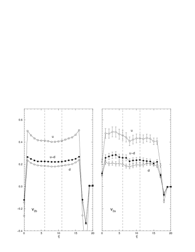
Figure 2: The ratio $R$, normalised so that when the conditions $0\ll\tau\ll t\mathrel{\hbox to0.0pt{\lower 4.0pt\hbox{\hskip 1.0pt$\sim$}\hss}\raise 1.0pt\hbox{$<$}}\mbox{\small$\frac{1}{2}$}N_{T}$ are met, the resulting plateau gives the bare matrix element. The picture shows the results for quenched $O(a)$-improved fermions at $\beta=6.20$ and $\kappa=0.1344$ on a $N_{S}^{3}\times N_{T}\equiv 24^{3}\times 48$ lattice. $t=17$ and a typical fit range for the plateau is taken from $\tau=6$ to $11$, shown by vertical dashed lines. The LH picture shows the ‘diagonal’ representation, $v_{2b}$ with a stationary nucleon, while the RH picture shows the ‘off-diagonal’ representation $v_{2a}$, which requires a moving nucleon with (lowest possible) momentum $\vec{p}=\vec{p}_{1}\equiv(2\pi/N_{S},0,0)$. The empty symbols refer to $u$ and $d$ matrix elements, while the full symbols give the NS matrix elements.

Due to the increase in noise in the signal, it is clearly advantageous to take a stationary nucleon – but this is unfortunately only possible for the lowest moments.

The operators (or raw results) must be renormalised. If using $O(a)$-improved Wilson type fermions, one also wishes to improve the operator. At present these additional operators are known for local (ie no $D$) and one-link (ie one $D$) operators [30], but not for higher-link operators. Numerically when known these additional operators do not seem to be significant, [31]. Perturbatively $Z$ is known for all the local operators, and for the one-link operators, [30]. For the higher-link operators only the unimproved results are presently known. For Ginsparg-Wilson (GW) fermions, the situation is simpler as the improvement coefficients are simple numbers, [32], while the renormalisation constants are given in [33]. Furthermore renormalisation constants for local operators for Domain Wall (DW) fermions have also been calculated in [34].

As most of the perturbative one-loop coefficients are known, then tadpole improvement (TI) of the renormalisation constants is possible. There are several variants, the one we shall use here is given in [35]. Here the renormalisation group invariant form of the renormalisation constant is directly computed. This can then be converted into the conventional $\overline{MS}$-scheme.

Non-perturbative renormalisation has also been attempted using both the Schrödinger Functional (SF) method, and the RI-MOM-scheme. The SF method was developed mainly by the ALPHA collaboration, and presently in quenched QCD most of the improvement coefficients and renormalisation constants for $O(a)$-improved Wilson fermions for the local operators are known, [36, 37], while for one-link operators ($v_{2a}$) the renormalisation constant has been determined for both unimproved and $O(a)$-improved fermions, [38]. An alternative approach, RI-MOM, based on generalising the perturbative procedure for the determination of the renormalisation constants has been applied to local, [39, 40], and higher link operators, [40, 35], for unimproved Wilson fermions. For $O(a)$ improved Wilson fermions local [41] and one-link operators [42] have been investigated. For DW fermions $Z$ for local operators have been found in [43]. For unquenched fermions, very little is known at present, [44]. However as we later want to compare quenched and unquenched results, we shall use for consistency the TI Z (except for $Z_{a_{0}}$, [42]).

Finally the operator mixing renormalisation structure is partially known. There is possible additional mixing with operators of the same dimension for $v_{3}$ and $v_{4}$, [29]. Also mixing with lower dimensional operators occurs, in particular for $d_{2}$, [45], and $d_{1}$. These are due to additional chiral non-invariant operators which occur for Wilson fermions (but not for DW or GW fermions). This point will be discussed further in section 6.1. Also the formalism for the SF method has been developed for singlet operators mixing with gluon operators, [46].

3 CHIRAL AND CONTINUUM EXTRAPOLATIONS

The next step is to attempt a chiral extrapolation. An example for quenched $O(a)$-improved Wilson fermions for $v_{2b}$ is shown in Fig. 3.

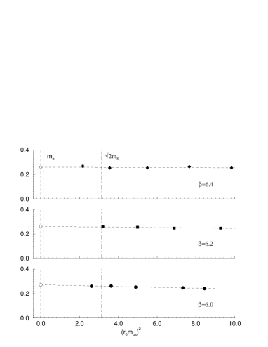
Figure 3: $v_{2b;NS}^{\mbox{\tiny$\overline{MS}$}}(2\mbox{GeV})$ versus $(r_{0}m_{ps})^{2}\sim r_{0}m_{q}$ using $\beta=6.0$, $6.2$ and $6.4$ for $O(a)$-improved quenched Wilson fermions. For orientation, the dash-dotted lines represents (roughly) a strange pseudoscalar meson ($m_{s}$ quark mass, determined from $m_{K}$), and the long-dashed line to the pion ($ud$ quark mass). The chiral limit is given by the short dashed lines. Also shown is a linear extrapolation.

The points have been scaled to $\overline{MS}$ at $\mu=2.0\mbox{GeV}$ (using $r_{0}=0.5\mbox{fm}\sim(400\mbox{MeV})^{-1}$). Also shown is a linear extrapolation to the chiral limit,

$$v_{n;NS}=a_{n}(r_{0}m_{ps})^{2}+b_{n}$$

which seems to be adequate, but one should remember that all the data points lie at the strange quark mass or higher. For $v_{3}$ and $v_{4}$ similar extrapolations can be performed, but as they need a moving nucleon yield much more noisy signals.

Finally to obtain the phenomenological result, an extrapolation to the continuum limit must be performed. These extrapolations are shown in Fig. 4 for $v_{2}$, $v_{3}$ and $v_{4}$.

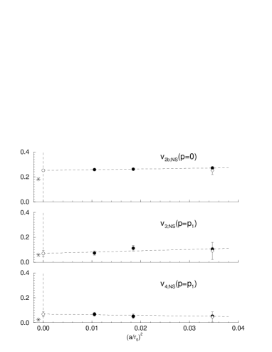
Figure 4: The continuum extrapolation for $v_{2b;NS}^{\mbox{\tiny$\overline{MS}$}}$ at a scale of $2\mbox{GeV}$ using the results from Fig. 3, filled circles with the linear extrapolated result being given by the empty circle. Also shown is the LHPC+SESAM result, [20] using unimproved Wilson fermions, empty diamond. The stars are the MRS phenomenological values, [47].

One can see the degradation of the signal as one goes to the higher moments, which makes the continuum extrapolation rather noisy. At least for $v_{2b}$ one can say that lattice effects appear to be small. Also shown is the result from [20] for unimproved Wilson fermions. Good agreement is seen, which again tends to suggest that lattice effects are small. The results of the extrapolation are also compared to the phenomenological MRS results, [47]. It is at present difficult to make any definite statement about the higher moments $v_{3}$ and $v_{4}$ except to say that due to the continuum extrapolation the ordering has been inverted (we would expect $v_{3}>v_{4}$). The problem seems to lie in the continuum extrapolation and can only be cured with more $\beta$-values. For $v_{2}$ three $\beta$ values seem to be sufficient; but the extrapolated result then seems to be about $30\%$ higher than the phenomenological value.

One might be worried that one should perform the continuum extrapolation before the chiral extrapolation. The previous fits can be thought of as finding the best $\beta$-$(r_{0}m_{ps})^{2}$ plane to the data, so a variant procedure is to try a joint fit, [48],

$$v_{2b;NS}=a_{2}(r_{0}m_{ps})^{2}+b_{2}+c_{2}(a/r_{0})^{2}+d_{2}ar_{0}m_{ps}^{2}$$

where the first two parameters represent the ‘chiral physics’, the third parameter potential $O(a^{2})$ effects and the fourth parameter $\propto am_{q}\sim ar_{0}m_{ps}^{2}$ is to account for any residual quark mass effects. (With three $\beta$ values, one actually reduces the number of free parameters by one.) In Fig. 5 we show the results of this type of fit. The same continuum result is obtained.

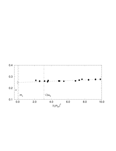
Figure 5: $v_{2b;NS}^{\mbox{\tiny$\overline{MS}$}}(2\mbox{GeV})$ with lattice artifacts removed, ie $v_{2b}-c_{2}(a/r_{0})^{2}-d_{2}ar_{0}m_{ps}^{2}$ showing the chiral extrapolation for the quenched $O(a)$-improved Wilson results of Figs. 3 and 4. The same notation as in Fig. 3.

4 UNQUENCHED RESULTS VERSUS QUENCHED RESULTS

One possible explanation for the discrepancy between the lattice result for $v_{2}$ and the phenomenological result is the use of the quenched approximation. Indeed one might expect that due to the momentum sum rule the quenched result is greater than the unquenched result (as the sea term part is suppressed in the quenched approximation). While most of the data at present uses quenched fermions, some recent results using unquenched fermions has appeared: from the LHPC and SESAM Collaboration, [20] (using unimproved Wilson fermions with $\beta=5.5$, $5.6$) and from the QCDSF and UKQCD Collaboration (using $O(a)$-improved Wilson fermions at $\beta=5.20$, $5.25$ and $5.29$, [35, 49]). (Both Collaborations have three quark mass values at each $\beta$ value.) Again, as in the quenched case, a linear chiral extrapolation (at fixed $\beta$) seems adequate. In Fig. 6

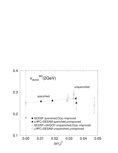
Figure 6: Quenched and unquenched results from the QCDSF+UKQCD and LHPC+SESAM Collaborations. Note that to determine $a$ different scales have been used (either $r_{0}$ or $m_{N}$ being extrapolated to the chiral limit), and also slightly different renormalisation procedures.

we plot the results against $(a/r_{0})^{2}$. Are there quenching effects? Although the unquenched results are not as good as the quenched results, it seems that in this quark mass ($\mathrel{\hbox to0.0pt{\lower 4.0pt\hbox{\hskip 1.0pt$\sim$}\hss}\raise 1.0pt\hbox{$>$}}m_{s}$) and $a$ range quenching effects are small.

Further quantities that have been considered include the axial charge (ie Bjorken Sum rule)

$$\int_{0}^{1}dxg_{1}^{p-n}(x,Q^{2}) = \mbox{\small$\frac{1}{6}$}E_{g_{1};a_{0};NS}\,g_{A}$$

$$\langle N(\vec{p},\vec{s})|\overline{q}\gamma^{\mu}\gamma_{5}q|N(\vec{p},\vec{s})\rangle = 2s^{\mu}\Delta q$$

with $\Delta u^{\mbox{\tiny$\overline{MS}$}}(\mu)-\Delta d^{\mbox{\tiny$\overline{MS}$}}(\mu)=g_{A}$ and the tensor charge

$$\int_{0}^{1}dxh_{1}^{p-n}(x,Q^{2}) = E^{\mbox{\tiny$\overline{MS}$}}_{h_{1};t_{0};NS}\,t^{\mbox{\tiny$\overline{MS}$}}_{0;NS}$$

$$\langle N(\vec{p},\vec{s})|\overline{q}i\sigma^{\mu\nu}\gamma_{5}q|N(\vec{p},\vec{s})\rangle = {2\over m_{N}}(s^{\mu}p^{\nu}-s^{\nu}p^{\mu})\delta q$$

with $\delta u^{\mbox{\tiny$\overline{MS}$}}(\mu)-\delta d^{\mbox{\tiny$\overline{MS}$}}(\mu)=t_{0;NS}^{\mbox{\tiny$\overline{MS}$}}(\mu)$. In Figs. 7 and 8

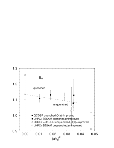
Figure 7: Quenched and unquenched results from the QCDSF+UKQCD and LHPC+SESAM Collaborations, for $g_{A}$ using the same notation as in Fig. 6.

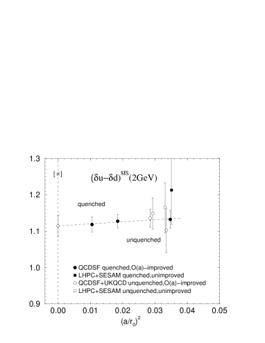
Figure 8: Quenched and unquenched results from the QCDSF+UKQCD and LHPC+SESAM Collaborations, for $(\delta u-\delta d)^{\mbox{\tiny$\overline{MS}$}}(\mu)$ using the same notation as in Fig. 6.

we show equivalent pictures to Fig. 6. Again little difference between the quenched and unquenched simulations is seen.

5 TOWARDS SMALL QUARK MASSES

The results shown previously have all been characterised by having data points at quark masses at or above the strange quark mass, and then a linear extrapolation in the quark mass to the chiral limit. There has been much recent work developing chiral perturbation theory, $\chi$-PT, [50, 51, 52, 53] which has shown the existence of a chiral logarithm of the form $\sim m_{q}\ln m_{q}$,

$$t_{n;NS} = T_{n}(1-\mbox{\small$\frac{1}{2}$}C_{4}m_{ps}^{2}\ln(m_{ps}^{2}/\mu_{\chi}^{2}))$$

$$v_{n;NS} = V_{n}(1-C_{3}m_{ps}^{2}\ln(m_{ps}^{2}/\mu_{\chi}^{2}))$$

$$a_{n;NS} = A_{n}(1-C_{2}m_{ps}^{2}\ln(m_{ps}^{2}/\mu_{\chi}^{2}))$$

where $C_{n}=(ng_{A}^{2}+1)/(4\pi f_{\pi})^{2}$ for (full) QCD. For quenched QCD an expression for $C_{3}$ in terms of $F$ and $D$ constants can be found in [54]. (Note that for quenched QCD for the nucleon there is no ‘hairpin’ contribution giving rise to the logarithm $\sim\ln m_{q}$ for $v_{n}$.) What is a suitable value for the chiral scale $\mu_{\chi}$? Roughly for $m_{ps}>\mu_{\chi}$, pion loops are suppressed and there is a linear variation in $m_{q}$ ie constituent quark behaviour, while for $m_{ps}<\mu_{\chi}$ we have non-linear behaviour. Often a value for $\mu_{\chi}\sim 1\mbox{GeV}$ is taken. We shall also use a comparison value of $500\mbox{MeV}$ here. From the above formulae, we see that $\chi$-PT always decreases the value of the matrix element as $m_{ps}^{2}\to 0$. Thus the lattice result should always be larger than the $\chi$-limit result. Also we would expect more effect for $v_{n}$ than for $a_{n}$. (Recent work in [55] indicates however that when including $\Delta$ as well as the $N$ then effectively bending only occurs for $v_{n}$ but not $a_{n}$ and $t_{n}$.)

As it is not so clear to which quark mass $\chi$-PT is valid, and as the results shown so far at $m_{q}\mathrel{\hbox to0.0pt{\lower 4.0pt\hbox{\hskip 1.0pt$\sim$}\hss}\raise 1.0pt\hbox{$>$}}m_{s}$ yield a linear behaviour it is necessary to go to lower quark masses. In [35] this was started using unimproved quenched Wilson fermions at $\beta=6.0$ (as the problem of ‘exceptional configurations’ then seems to be less severe). The present status, [56], is shown in Fig. 9.

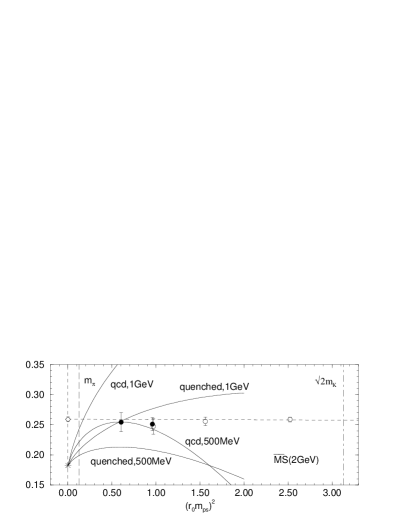
Figure 9: Quenched results for unimproved Wilson fermions at $\beta=6.0$ for $v_{2b;NS}^{\mbox{\tiny$\overline{MS}$}}(2\mbox{GeV})$. The empty circles are for heavier quark masses on a $24^{3}\times 32$ lattice, $O(200)$ configurations, while the filled circles for the lighter quark masses are on a $32^{3}\times 48$ lattice, $O(100/50)$ configurations, [56]. Finite volume effects are checked at the second lightest mass. The dashed line is a linear fit to the data. From the MRS value (star), [47], the $\chi$-PT formula is applied, with $C_{3}/r_{0}^{2}\sim 0.28$, $0.67$ for quenched or full QCD respectively and for two values of the chiral scale $\mu_{\chi}$.

All quark masses have $am_{ps}N_{S}\mathrel{\hbox to0.0pt{\lower 4.0pt\hbox{\hskip 1.0pt$\sim$}\hss}\raise 1.0pt\hbox{$>$}}4$. As $(r_{0}2m_{\pi})^{2}\sim 0.5$, the lightest mass used in the simulation is $\sim 2m_{ud}$ (this corresponds to $m_{ps}/m_{V}\sim 0.4$). Little curvature in the numerical results is seen, but is still possible, as we expect the coefficient $C_{3}$ to be smaller than in the unquenched case, [54]. Also, as noted before, quenching might give a higher value for $v_{2b}$ than the phenomenological value anyway.

In Fig. 10 we show results for $g_{A}$.

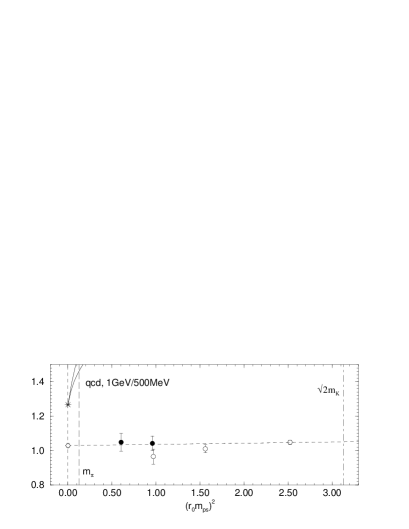
Figure 10: Quenched results for unimproved Wilson fermions at $\beta=6.0$ for $g_{A}$. Notation as in Fig. 9.

Note that $\chi$-PT goes in the wrong direction. It is less clear if there is a finite volume effect. Ref. [57] suggested that the charge is delocalised in the chiral (and infinite volume) limit, $g_{A}\to 2/3g_{A}$. This was further discussed in [58], which showed that for finite volumes, there are no (large) volume effects.

Nevertheless the questions of finite volume effects and the range of applicability for Wilson fermions near the chiral limit remain, and recently there have also been results using DW fermions by the RBC Collaboration. These have much better chiral properties than Wilson fermions and so are more suitable for investigating small quark masses. In [59], $v_{2b}$ is computed on a $16^{3}\times 32[\times 16]$ lattice at $a^{-1}\sim 1.3\mbox{GeV}$. Thus the lowest pion mass there, $(am_{ps})^{2}\sim 0.1$, corresponds to about $(r_{0}m_{ps})^{2}\sim 1$ in Fig. 9. At this point some curvature in the signal is present. For $g_{A}$, [60], finite volume effects are seen. Thus the general situation is not completely clear.

6 OTHER TOPICS

6.1 Non-perturbative mixing

A further source of discrepancy between lattice results and phenomenological results can lie in the incorrect treatment of non-perturbative mixing of the lattice operators. An example is given by $d_{2}$, which can be found from $g_{2}$,

$$\int_{0}^{1}dxx^{2}g_{2}(x,Q^{2}) = \mbox{\small$\frac{1}{6}$}\sum_{q=u,d}\left[E^{(q)}_{d_{2}}d_{2}^{(q)}-E^{(q)}_{a_{2}}a_{2}^{(q)}\right]$$

$$\int_{0}^{1}dxx^{2}g_{1}(x,Q^{2}) = \mbox{\small$\frac{1}{4}$}\sum_{q=u,d}E^{(q)}_{a_{2}}a_{2}^{(q)}$$

where $a_{2}$ and $d_{2}$ are given in section 1 as nucleon matrix elements of certain operators ${\cal O}^{(q)}_{a_{2}/d_{2}}\sim\overline{q}\gamma\gamma_{5}DDq$. The $a_{n}$ operators have twist two, but $d_{n}$ corresponds to twist three and is thus of particular interest. A ‘straightforward’ lattice computation, [19, 20], gave rather large values for $d_{2}^{p}$. A recent experiment, [8], however indicated that this term was very small. This problem was traced in [45] to a mixing of the original operator ${\cal O}^{(q)}_{d_{2}}$ with a lower-dimensional operator ${\cal O}_{\sigma}^{(q)}\sim\overline{q}\sigma Dq$. This additional operator mixes $\propto 1/a$ and so its renormalisation constant must be determined non-perturbatively. In [45] this was attempted using RI-MOM, and led to results qualitatively consistent with the experimental values. Note that this is only a problem when using Wilson-like fermions, as we would expect the operator to appear like $\sim m_{q}\overline{q}\sigma Dq$ and hence vanish in the chiral limit. Thus there should be no mixing if one uses GW or DW fermions. In [59] this was investigated for $d_{1}$ using DW fermions and compared with unimproved Wilson fermions $d_{1}$ results from [20]. The same phenomenon was seen: $d_{1}$ using DW fermions gave a small value in the chiral limit, while the unimproved Wilson fermion results increased strongly as the quark mass was reduced.

6.2 Higher Twist effects

Potential higher twist effects are present in the moment of a structure function, see section 1. These $O(1/Q^{2})$ terms have four quark matrix elements. A general problem is the non-perturbative mixing of these new dimension 6 operators with the previous dimension 4 operators. At present results are restricted to finding combinations of these higer twist operators which do not mix from flavour symmetry. In [61] the lowest moment of the pion structure function was considered,

$$\int_{0}^{1}dxF_{2}(x,Q^{2})|^{I=2}_{Nachtmann}=$$

$$1.67(64){f_{\pi}^{2}\alpha_{s}(Q^{2})\over Q^{2}}+O(\alpha_{s}^{2})$$

where the $SU_{F}(2)$ flavour symmetry group gives the combination $F_{2}^{I=2}=F_{2}^{\pi^{+}}+F_{2}^{\pi^{-}}-2F_{2}^{\pi^{0}}$. For the nucleon the $SU_{F}(3)$ flavour symmetry group must be considered, ie taking mass degenerate $u$, $d$ and $s$ quarks, [62], giving

$$\int_{0}^{1}dxF_{2}(x,Q^{2})|^{27,I=1}_{Nachtmann}=$$

$$-0.0005(5){m_{p}^{2}\alpha_{s}(Q^{2})\over Q^{2}}+O(\alpha_{s}^{2})$$

(To access this moment experimentally needs the measurement of structure functions of $p$, $n$, $\Lambda$, $\Sigma$ and $\Xi$ baryons.) These results are for quenched unimproved Wilson fermions at $\beta=6.0$, and are very small in comparison with the leading twist result. However these are rather exotic combinations of matrix elements and say little about individual contributions. Nevertheless this might hint that higher twist contributions are small.

6.3 Pion, Rho and Lambda results

Moments for pion and rho structure functions were computed in [63], for unimproved Wilson fermions. Using the SF method, $v_{2a}$ was calculated for the pion, [64] for both unimproved and $O(a)$-improved fermions, giving numbers in agreement with [63]. Finally there have been results for moments of $\Lambda$ structure functions, [65]. These are potentially useful as one can compare with nucleon spin structure and check violation of $SU_{F}(3)$ symmetry. First indications are that there is little flavour symmetry breaking.

7 CONCLUSIONS AND FUTURE PERSPECTIVES

Clearly the computation of many matrix elements giving low moments of structure functions is possible. We would like to emphasise that a successful computation is a fundamental test of QCD – this is not a model computation. There are however many problems to overcome: finite volume effects, renormalisation and mixing, continuum and chiral extrapolations and unquenching. At present although overall impressions are encouraging, still it is difficult to re-produce experimental/phenomenological results of (relatively) simple matrix elements (eg $v_{2}$, $g_{A}$). Improvements are thus necessary in all areas. Nevertheless progress is being made: there are now considerations of both chiral and continuum extrapolations, some dynamical results are now available, there are attempts to understand lower quark mass both numerically (using both Wilson fermions and DW fermions) and from $\chi$-PT. Clearly everything depends on the data and the quest for better results should continue. To leave the region where constituent quark masses give a reasonable description of the data, seems unfortunately to require quark masses rather close to the $ud$ mass. This will presumably also entail the use of unquenched chiral fermions (such as GW/DW). This will need much faster machines and is, perhaps, a cautionary tale for the determination of other matrix elements.

References

- [1] J. Blümlein et al., Nucl. Phys. B498 (1997) 285, hep-ph/9612318.
- [2] V. Barone et al., Phys. Rept. 359 (2002) 1, hep-ph/0104283.
- [3] A. M. Cooper-Sarkar et al., Int. J. Mod. Phys. A13 (1998) 3385, hep-ph/9712301.
- [4] A. T. Doyle, hep-ex/9812029.
- [5] H1 Collaboration, eg hep-ex/0206062.
- [6] Zeus Collaboration, eg hep-ex/0208040.
- [7] Hermes Collaboration, eg Phys. Lett. B464 (1999) 123, hep-ex/9906035.
- [8] E155 Collaboration, Phys. Lett. B458 (1999) 529, hep-ex/9901006.
- [9] C. S. Armstrong et al., Phys. Rev. D63 (2001) 094008, hep-ph/0104055.
- [10] I. Niculescu et al., Phys. Rev. Lett.85 (2000) 1182; ibid 1186.
- [11] Compass Collaboration, eg hep-ex/9611016.
- [12] CCFR Collaboration, eg Phys. Rev. Lett. 86 (2001) 2742, hep-ex/0009041.
- [13] G. Bunce et al., Ann. Rev. Nucl. Part. Sci. 50 (2000) 525, hep-ph/0007218.
- [14] eg DIS2002, April 2002, Krakow, Poland.
- [15] O. Nachtmann, hep-ph/0206284.
- [16] S. Caracciolo et al., JHEP 0009 (2000) 045, hep-lat/0007044.
- [17] S. Capitani et al., Nucl. Phys. Proc. Suppl. 79 (1999) 173, hep-ph/9906320.
- [18] Spin Muon Collaboration (SMC), Phys. Lett. B420 (1998) 180, hep-ex/9711008.
- [19] M. Göckeler et al., Phys. Rev. D53 (1996) 2317, hep-lat/9508004.
- [20] D. Dolgov et al., Phys. Rev. D66 (2002) 034506, hep-lat/0201021.
- [21] M. Göckeler et al., Phys. Lett. B414 (1997) 340, hep-ph/9708270.
- [22] S. Aoki et al., Phys. Rev. D56 (1997) 433, hep-lat/9606006.
- [23] S. Capitani et al., Nucl. Phys. Proc. Suppl. 79 (1999) 548, hep-ph/9905573.
- [24] G. Martinelli, Nucl. Phys. Proc. Suppl. 9 (1989) 134.
- [25] M. Göckeler et al., Nucl. Phys. Proc. Suppl. 53 (1997) 81, hep-lat/9608046.
- [26] G. Martinelli et al., Nucl. Phys. B316 (1989) 355.
- [27] M. Okawa, Nucl. Phys. Proc. Suppl. 47 (1996) 160, hep-lat/9510047.
- [28] S. Güsken, hep-lat/9906034.
- [29] M. Göckeler et al., Phys. Rev. D54 (1996) 5705, hep-lat/9602029.
- [30] S. Capitani et al., Nucl. Phys. B593 (2001) 183, hep-lat/0007004.
- [31] S. Capitani et al., in preparation.
- [32] S. Capitani et al., Phys. Lett. B468 (1999) 150, hep-lat/9908029.
- [33] S. Capitani, Nucl. Phys. B592 (2001) 183, hep-lat/0005008; Nucl. Phys. B597 (2001) 313, hep-lat/0009018.
- [34] S. Aoki et al., Phys. Rev. D59 (1999) 094505, hep-lat/9810020.
- [35] S. Capitani et al, Nucl. Phys. Proc. Suppl. 106 (2002) 299, hep-lat/0111012.
- [36] M. Lüscher et al., Nucl. Phys. B491 (1997) 344, hep-lat/9611015.
- [37] S. Capitani et al., Nucl. Phys. B544 (1999) 669, hep-lat/9810063.
- [38] M. Guagnelli et al., Phys. Lett. B459 (1999) 594, hep-lat/9903012; Phys.Lett. B493 (2000) 77, hep-lat/0009006.
- [39] G. Martinelli at al., Nucl. Phys. B445 (1995) 81, hep-lat/9411010.
- [40] M. Göckeler et al., Nucl. Phys. B544 (1999) 699, hep-lat/9807044.
- [41] V. Lubicz, talk at this conference.
- [42] M. Göckeler et al., in preparation.
- [43] T. Blum et al., Phys. Rev. D66 (2002) 014504, hep-lat/0102005.
- [44] R. Horsley, Nucl. Phys. Proc. Suppl. 94 (2001) 307, hep-lat/0010059.
- [45] M. Göckeler et al., Phys. Rev. D63 (2001) 074506, hep-lat/0011091.
- [46] F. Palombi et al., hep-lat/0203002.
- [47] A. D. Martin et al., Phys. Lett. B354 (1995) 155, hep-ph/9502336.
- [48] S. Booth et al., Phys. Lett. B519 (2001) 229, hep-lat/0103023.
- [49] T. Bakeyev et al., talk, hep-lat/0209148.
- [50] W. Detmold et al., Phys. Rev. Lett. 87 (2001) 172001, hep-lat/0103006.
- [51] D. Arndt et al., Nucl. Phys. A697 (2002) 429, nucl-th/0105045.
- [52] J. Chen et al., Phys. Lett. B523 (2001) 107, hep-ph/0105197.
- [53] A. W. Thomas, plenary talk, hep-lat/0208023.
- [54] J. Chen et al., nucl-th/0108042.
- [55] W. Detmold et al., hep-lat/0206001.
- [56] M. Göckeler et al., poster, hep-lat/0209151.
- [57] R. L. Jaffe, Phys. Lett. B529 (2002) 105, hep-ph/0108015.
- [58] T. D. Cohen, Phys. Lett. B529 (2002) 50, hep-lat/0112014.
- [59] K. Orginos, talk, hep-lat/0209137.
- [60] S. Ohta, poster at this conference.
- [61] S. Capitani et al., Nucl. Phys. B570 (2000) 393, hep-lat/9908011.
- [62] M. Göckeler et al., Nucl. Phys. B623 (2002) 287, hep-lat/0103038.
- [63] C. Best et al., Phys. Rev. D56 (1997) 2743, hep-lat/9703014.
- [64] K. Jansen, hep-lat/9903012.
- [65] M. Göckeler et al., hep-lat/0208017.