Mass gap in compact U(1) Model in (2+1) dimensions
Abstract
A numerical study of low-lying glueball masses of compact U(1) lattice gauge theory in (2+1) dimensions is performed using Standard Path integral Monte Carlo techniques. The masses are extracted, at fixed (low) temperature, from simulations on anisotropic lattices, with temporal lattice spacing much smaller than the spatial ones. Convincing evidence of the scaling behaviour in the antisymmetric mass gap is observed over the range . The observed behaviour is very consistent with asymptotic form predicted by Göpfert and Mack. Extrapolations are made to the “Hamiltonian” limit, and the results are compared with previous estimates obtained by many other Hamiltonian studies.
I Introduction
Compact U(1) lattice gauge theory in three-dimensions is the most well-understood nontrivial gauge theory. The theory exhibits some important similarities with QCD [16], such as confinement [2, 3] and chiral symmetry breaking [4]. Because of its simplicity, it has been a good testing ground for new methods and algorithmic approaches. While the Euclidean Path Integral Monte Carlo simulations [5] have been very successful in the study of non-perturbative lattice gauge theories and is currently the preffered technique for studying QCD at low energies, there there has been some progress in the development of analytic and numerical approaches in the Hamiltonian formalism. The Hamiltonian version of the model has been studied by many methods: some recent studies include series expansions [6], finite-lattice techniques[7], the t-expansion [8, 9], and coupled-cluster techniques [10, 11, 12], as well as Quantum Monte Carlo methods[13, 14, 15, 16, 17, 18, 19]. Quite accurate estimates have been obtained for the string tension and the mass gaps, which can be used as comparison for our present results. The finite-size scaling properties of the model can be predicted using an effective Lagrangian approach combined with a weak-coupling expansion [20], and the predictions agree very well with finite-lattice data [16]. Here our aim is to use standard Euclidean path integral Monte Carlo techniques for an anisotropic lattice, and see whether useful results can be obtained in the anisotropic or Hamiltonian limit.
II Compact U(1) Model in 3 Dimensions
The anisotropic Wilson gauge action for compact U(1) model in (2+1) dimensions has the form [21]
| (1) |
Where and are the spatial and temporal plaquette variables respectively. In the classical limit
| (2) | |||||
| (3) |
where ( in (2+1)D)) and is the anisotropy parameter, is the lattice spacing in the space direction, and is the temporal spacing. In the weak-coupling approximation, the above action can be written as
| (4) |
In the limit , the time variable becomes continuous and one obtains the Hamiltonian limit of the model (modulo a Wick rotation back to Minkowski space).
Among other features, antisymmetric mass gap is a fundamental quantity of interest in U(1) model. On an isotropic lattice, the model reduces to the simple continuum theory of non-interacting photons in the naive continuum limit at a fixed energy scale [22] but if one renormalizes or rescales in the standard way so as to maintain the mass gap constant, then one obtains a confining theory of free massive bosons. Göpfert and Mack[23] proved that in the continuum limit the theory converges to a scalar free field theory of massive bosons. They found that in that limit the mass gap behaves as
| (5) |
where is the Coulomb potential at zero distance for the isotropic case.
The behaviour of the mass gap in the anisotropic case will be similar to equation (5) Generalizing discussions by Banks et al[24] and Ben-Menahem[25], we find that the exponential factor takes exactly the same form in the anisotropic case. The only difference is that the lattice Coulomb potential at zero spacing for general is
| (6) | |||||
| (9) |
The above result is based on dilute gas approximation, which is justified in the Euclidean case, but not in the Hamiltonian limit[24, 25].
The expected finite-size scaling behaviour of the mass gap near the continuum critical point in this model is not known; but Weigel and Janke[26] have performed a Monte Carlo simulation for an O(2) spin model in three dimensions which should lie in the same universality class, obtaining
| (10) |
for the magnetic gap.
III Monte Calro simulations and glueball masses
Using the anisotropic Wilson action, we perform Monte Carlo simulations on a finite lattice of size , where is the number of lattice sites in the space direction and in the temporal direction, with spacing ratio . By varying it is possible to change , while keeping the spacing in the spatial direction fixed. The details of the algorithm for updating are given elsewhere [27]. The simulations were performed on lattices with sites in each of the two spatial directions and in the temporal direction for a range of couplings .
IV Results and Discussion
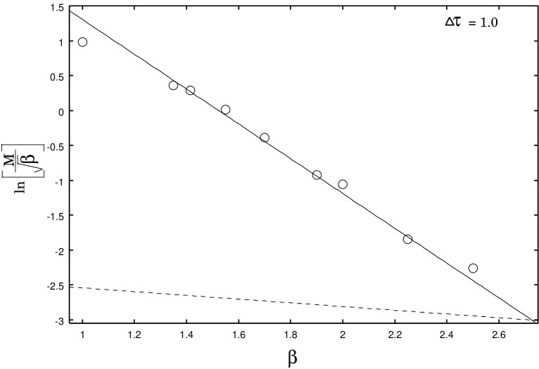
Figure 1 shows the estimates for the glueball masses of and channels against for the Euclidean case . As expected the masses are seen to vanish exponentially with as we approach the continuum limit (high ). To show the evidence of scaling behaviour of antisymmetric glueball masses , we used the predicted asymptotic form, equation 5, with an additional normalization constant;
| (11) |
where when adjusted to fit the data. Figure 2 shows the predicted scaling behaviour. The solid line on the graph is a fit to the data over the range . The slope, , of the data matches the predicted asymptotic form very nicely, but the coefficient is too large by a factor of 5.2. It would again be interesting to explore whether this discrepancy could be due to quantum corrections. The finite-size scaling behaviour is shown by the dashed line in Figure 2. It can be seen that the Euclidean mass gap should not be effected by finite-size corrections until .
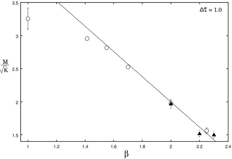
To check the consistency of our method, we plot the dimensionless ratio of the the antisymmetric mass gap over the square root of the string tension against together with the results of Teper [29] in Figure 3. The agreement is excellent. The solid line gives the ratio of the fits in Figures 2 and Fig. (8) in [28], and shows how this ratio vanishes exponentially in the weak-coupling limit, whereas in four-dimensional confining theories it goes to a constant.
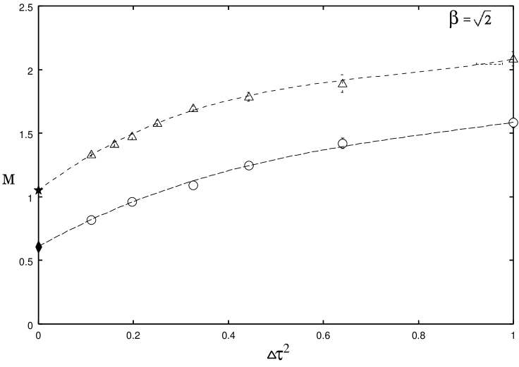
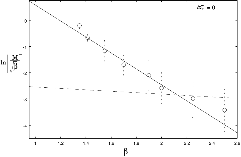
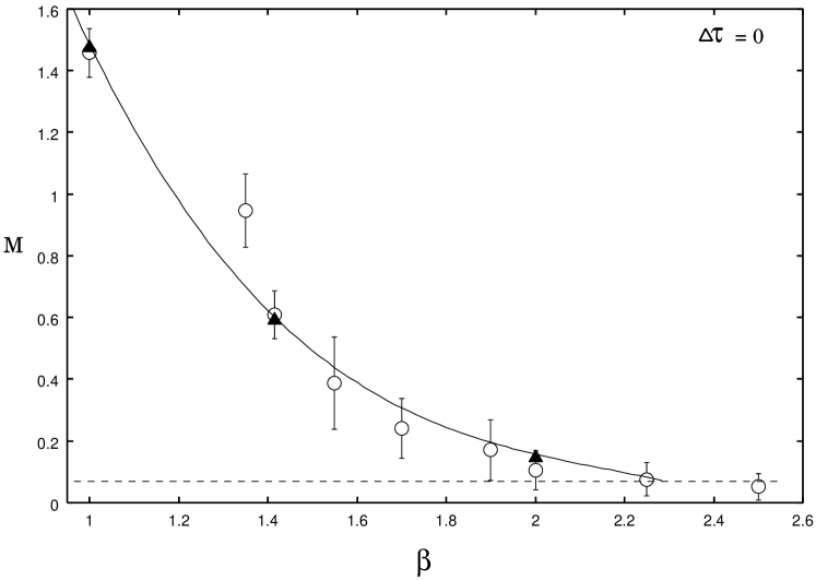
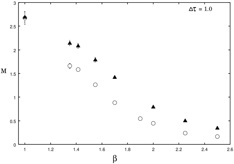
Figure 4 shows the behaviour of the glueball masses as function of for . The extrapolation to the Hamiltonian limit is performed by a simple cubic fit in powers of . In the limit , we reproduce the earlier series estimates of Hamer et al[6] for the and states. The estimates of the antisymmetric mass gap, for various , extracted from the extrapolation to the limit are graphed as a function of in Figure 5. The solid line is a fit to the data for of the form (5), with and , which is similar to the coefficient found in the Euclidean case. The fitting parameters, the slope, and the intercept, , of the scaling curve are in excellent agreement with the results obtained from the other Hamiltonian studies and are listed in table I. The dashed line represents the finite-size scaling behaviour, equation (10), which we assume holds in the Hamiltonian limit also, for want of better information. It can be seen that the finite-size corrections are predicted to dominate for , but the date are not accurate enough at weak couplings to establish whether this is really the case. Figure 6 shows the our Monte Carlo estimates for antisymmetric mass gap as a function of . Also are shown the results from previous strong-coupling series extrapolations[6] and quantum Monte Carlo calculations[16]. It can be seen that our present results agree with previous estimates but are less accurate.
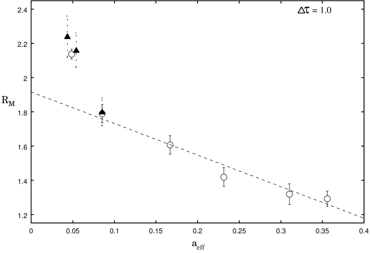
Finally, Figure 7 displays the behaviour of the dimensionless mass ratio,
| (12) |
for the Euclidean case . As in the (3+1)D confining theories, we may expect that quantities of this sort will approach their weak-coupling or continuum limits with corrections of , where is the effective lattice spacing in ‘physical’ units when the mass gap has been renormalized to a constant. Hence for our present purposes we define from equation (5) as
| (13) |
with for the Euclidean case. The mass ratio is plotted against in Figure 6. At weak coupling, we expect the theory to approach a theory of free bosons[23] so that the symmetric state will be composed of two bosons and the mass ratio should approach two. Our results show that as goes to zero, the mass ratio rises to around the expected value of . A linear fit to the data from gives an intercept However, we note that the last one of our estimates, together with two from Teper[29], lie considerably above . In the bluk systems, of course, the ratio cannot rise above 2, because it is always possible to construct a state out of two mesons. been included in the fit.
Acknowledgments
This work was supported by the Australian Research Council. We are grateful for access to the computing facilities of the Australian Centre for Advanced Computing and Communications (ac3) and the Australian Partnership for Advanced Computing (APAC).
REFERENCES
- [1] C. J. Hamer, K. C. Wang and P. F. Price, Phys. Rev. D50, 4693 (1994)
- [2] A.M. Polyakov, Phys. Lett. 72B, 477 (1978)
- [3] A.M. Polyakov, Nucl. Phys. 120B, 429 (1977)
- [4] H.R. Fiebig and R.M. Woloshyn, Phys. Rev. 120D, 3520 (1990)
- [5] M. Creutz, Phys. Rev. Letts. 43, 553 (1979)
- [6] C. J. Hamer, J. Oitmaa, and Zheng Weihong, Phys. Rev. D45, 4652 (1992)
- [7] A.C. Irving, J.F. Owens and C.J.Hamer, Phys. Rev. D28, 2059 (1983)
- [8] D. Horn, G. Lana and D. Schreiber, Phys. Rev. D36, 3218 (1987)
- [9] C.J. Morningstar, Phys. Rev. D46, 824 (1992)
- [10] A. Dabringhaus, M.L. Ristig and J.W. Clark, Phys. Rev. D43, 1978 (1991)
- [11] X.Y. Fang, J.M. Liu and S.H. Guo, Phys. Rev. D53, 1523 (1996)
- [12] S.J. Baker, R,.F. Bishop and N.J. Davidson, Phys. Rev. D53, 2610 (1996)
- [13] S. A. Chin, J. W. Negele and S. E. Koonin, Ann. Phys. (N.Y.) 157, 140 (1984)
- [14] S. E. Koonin, E. A. Umland and M. R. Zirnbauer, Phys. Rev. D33, 1795 (1986)
- [15] C. M. Yung, C. R. Allton and C. J. Hamer, Phys. Rev. D33, 1795 (1986)
- [16] C. J. Hamer, K. C. Wang and P. F. Price, Phys. Rev. D50, 4693 (1994)
- [17] J. McIntosh and L. Hollenberg, Z. Phys. C76, 175 (1997)
- [18] M.N. Chernodub, E.-M. Ilgenfritz and A. Schiller, Phys. Rev. bf 64D, 054507 (2001)
- [19] C.J. Hamer, R.J. Bursill and M. Samaras, Phys. Rev. D62, 054511 (2000)
- [20] C. J. Hamer and Zheng Weihong, Phys. Rev. D48, 4435 (1993)
- [21] C.J. Morningstar and M. Peardon, Phys. Rev. D56, 4043 (1997)
- [22] L. Gross, Commun. Math. Phys. 92, 137 (1983)
- [23] M. Göpfert and G. Mack, Commun. Math. Phys. 82, 545 (1982)
- [24] T. Banks, R. Myerson and J. Kogut, Nucl. Phys. B129, 493 (1977)
- [25] S. Ben-Menahem, Phys. Rev. D20, 1923 (1979)
- [26] M. Weigel and W. Janke, Phys. Rev. Letts. 82, 2318 (1999)
- [27] M. Loan et al., hep-lat/0209159
- [28] M. Loan et al., hep-lat/0208047
- [29] M.J. Teper, Phys. Rev. D59, 014512 (1999)
- [30] G. Lana, Phys. Rev. D38, 1954 (1988)
- [31] C.J. Hamer and A.C. Irving, Z. Phys. C27, 145 (1985)
- [32] D.W. Heys and D.R. Stump, Nucl. Phys. B257, 19 (1987)
- [33] F. Xiyan, L. Jinming and G. Shuohong, Phys. Rev. D53 1523 (1996)
- [34] A. Darooneh and M. Modarres, Eur. Phys. J. C17, 169 (2000)
| Source | ||
| Villain (Hamiltonian) | 3.17 | 2.18 |
| Lana [30] | 2.05 | 2.49 |
| Hamer and Irving [31] | 2.65 | 3.07 |
| Hamer, Oitmaa and Weihong [6] | 2.71 | 3.13 |
| Dabrighaus, Ristig and Clark [10] | 2.40 | 3.13 |
| Fang, Liu and Guo [11] | 2.50 | 2.94 |
| Morningstar [9] | 2.61 | 2.97 |
| Heys and Stump [32] | 2.48 | 3.13 |
| McIntosh and Hollenberg [17] | 2.50 | 2.91 |
| Xiyan, Jinming and Shuohong [33] | 2.50 | 2.95 |
| Darooneh and Modarres [34] | ||
| This work |
.