PATH INTEGRAL MONTE CARLO APPROACH TO THE U(1) LATTICE GAUGE THEORY IN (2+1) DIMENSIONS

Abstract

Path Integral Monte Carlo simulations have been performed for U(1) lattice gauge theory in (2+1) dimensions on anisotropic lattices. We extract the static quark potential, the string tension and the low-lying “glueball” spectrum. The Euclidean string tension and mass gap decrease exponentially at weak coupling in excellent agreement with the predictions of Polyakov and Göpfert and Mack, but their magnitudes are five times bigger than predicted. Extrapolations are made to the extreme anisotropic or Hamiltonian limit, and comparisons are made with previous estimates obtained in the Hamiltonian formulation.

I Introduction

Classical Monte Carlo simulationscre79 of the path integral in Euclidean lattice gauge theorywil74 have been very successful, and this is currently the preferred method for ab initio calculations in quantum chromodynamics (QCD) in the low energy regime. Monte Carlo approaches to the Hamiltonian version of QCD propounded by Kogut and Susskindkog75 have been less successful, however, and lag at least ten years behind the Euclidean calculations. Our aim in this paper is to see whether useful results can be obtained for the Hamiltonian version by using the standard Euclidean Monte Carlo methods for anisotropic latticesmor97 , and extrapolating to the Hamiltonian limit in which the time variable becomes continuous, i.e. the lattice spacing in the time direction goes to zero. The Hamiltonian version of lattice gauge theory is less popular than the Euclidean version, but is still worthy of study. It can provide a valuable check of the universality of the Euclidean resultsham96 , and it allows the application of many techniques imported from quantum many-body theory and condensed matter physics, such as strong coupling expansionsban77a , the t-expansionhor84 , the coupled-cluster methodguo88 , the plaquette expansion john97 , loop representation method aro93 , and more recently the density matrix renormalization groupbyr02 (DMRG). None of these techniques has proved as useful as Monte Carlo in (3+1) dimensions; but in lower dimensions they are more competitive.

A number of Quantum Monte Carlo methods have been applied to Hamiltonian lattice gauge theory in the past, with somewhat mixed results. A “Projector Monte Carlo” approachbla83 ; deg85 using a strong coupling representation for the gauge fields runs into difficulties for non-Abelian models, in that it requires Clebsch-Gordan coefficients for SU(3) which are not even known at high orders; and furthermore a version of the “minus sign problem” rears its headham94 . A Greens Function Monte Carlo approach was pioneered by Chin et alchi84 and Heys and Stumphey83 , which uses a weak coupling representation for the gauge fields. This approach can be used successfully for non-Abelian theories, and obtains estimates of parameters such as the string tension and glueball masses from the correlation functions in a similar fashion to Euclidean techniques. Unfortunately the approach requires the use of a “trial wave function” to guide random walkers in the ensemble towards the preferred regions of configuration spacekal66 . This introduces a variational element into the procedure, in that the results may exhibit a systematic dependence on the trial wave function. We have previously exploredsam99 ; ham00 ; ham00a a “forward-walking” techniqueliu74 ; whi79 for measuring the expectation values and the correlation functions, which should minimize this dependence; but calculations for the SU(3) Yang-Mills theory in (3+1) dimensions still showed an unacceptably strong sensitivity to the parameters of the trial wave functionham00a . For this reason, we are forced to look yet again for an alternative approach.

As mentioned above our aim in this paper is to use standard Euclidean path integral Monte Carlo techniques for anisotropic lattices, and see whether useful results can be obtained in the Hamiltonian limit. Morningstar and Peardonmor97 showed some time ago that the use of anisotropic lattices can be advantageous in any case, particularly for the measurement of glueball masses. We use a number of their techniques in what follows.

As a first trial of this approach, we treat the U(1) gauge model in (2+1)D, which is one of the simplest models with dynamical gauge degrees of freedom, and has also been studied extensively by other means (see Section II). Path integral Monte Carlo methods were applied to this model a long time ago by Hey and collaboratorsamb82 ; cod86 , but the techniques used at that time were not very sophisticated, and the results were rather qualitative. Very little has been done since then using this approach on this particular model, apart from a calculation by Irbäck and Peterson irb87 .

The rest of this paper is organised as follows. In section II we discuss the U(1) model in (2+1) dimensions in its lattice formulation, and outline some of the work done on it previously. The details of the simulations, including the generation of the gauge-field configurations, the construction of the Wilson loop operators and glueball operators, and the extraction of the potential and string tension estimates are described in section III. In section IV we present our main results for the mean plaquette, static quark potential, string tension and glueball masses. The static quark potential has not previously been exhibited for this model, as far as we are aware. Finally we make an extrapolation to the Hamiltonian limit, and comparisons are made with estimates obtained by other means in that limit. We find that indeed the PIMC method can give better results than other weak-coupling Monte Carlo methods, even in the Hamiltonian limit. Our conclusions are summarized in Sec. VI.

II THE U(1) MODEL

Consider the isotropic Abelian U(1) lattice gauge theory in three dimensions. The theory is defined by the actionwil74

$$S=\beta\sum_{r,\mu,\nu}\mbox{ReTr}P_{\mu\nu}$$ (1)

where

$$\mbox{P}_{\mu\nu}(r)=\left[1-ReTr\{\mbox{U}_{\mu}(r)\mbox{U}_{\nu}(r+\hat{\mu})\mbox{U}_{\mu}^{\dagger}(r+\hat{\nu})\mbox{U}_{\nu}^{\dagger}(r)\right\}]$$ (2)

is the plaquette variable given by the product of the link variables taken around an elementary plaquette. The link variable $\mbox{U}_{\mu}(r)$ is defined by

$$\mbox{U}_{\mu}(r)=\mbox{exp}[ieaA_{\mu}(r)]=\mbox{exp}[i\theta_{\mu}(r)]$$ (3)

where in the compact form of the model, $\theta_{\mu}(r)(=eaA_{\mu}(r))\in[0,2\pi]$ represents the gauge field on the directed link $r\rightarrow r+\hat{\mu}$. The parameter $\beta$ is related to the bare gauge coupling by

$$\beta=\frac{1}{g^{2}}$$ (4)

where $g^{2}=ae^{2}$, in (2+1) dimensions.

The lattice U(1) model in (2+1) dimensions has been studied by many authors, and possesses some important similarities with QCD (for a more extensive review, see for example ref. ham94 ). If one takes the “naive” continuum limit at a fixed energy scale, one regains the simple continuum theory of non-interacting photonsgro83 ; but if one renormalizes or rescales in the standard way so as to maintain the mass gap constant, then one obtains a confining theory of free massive bosons. Polyakovpol78 showed that a linear potential appears between static charges due to instantons in the lattice theory; and Göpfert and Mackgop82 proved that in the continuum limit the theory converges to a scalar free field theory of massive bosons. They found that in that limit the mass gap behaves as

$$am_{D}=\sqrt{\frac{8\pi^{2}}{g^{2}}}\exp(-\frac{\pi^{2}}{g^{2}}v(0))$$ (5)

while the string tension is bounded by

$$a^{2}\sigma\geq c\sqrt{\frac{g^{2}}{2\pi^{2}}}\exp(-\frac{\pi^{2}}{g^{2}}v(0))$$ (6)

where $v(0)$ is the Coulomb potential at zero distance, and has a value in lattice units

$$v(0)=0.2527$$ (7)

for the isotropic case. They argue that (6) represents the true asymptotic behaviour of the string tension, where the constant $c$ is equal to $8$ in classical approximation. The theory has a non-vanishing string tension for arbitrarily large $\beta$, similar to the behaviour expected for non-Abelian lattice gauge theories in four dimensions.

For an anisotropic lattice, the gauge action becomesmor97

$$S=\beta_{s}\sum_{r,i<j}P_{ij}(r)+\beta_{t}\sum_{r,i}P_{it}(r)$$ (8)

where $P_{ij}$ and $P_{it}$ are the spatial and temporal plaquette variables respectively. In the classical limit

$$\beta_{s} = \frac{a_{t}}{e^{2}a_{s}^{2}}=\frac{1}{g^{2}}\Delta\tau$$ (9)

$$\beta_{t} = \frac{1}{e^{2}a_{t}}=\frac{1}{g^{2}}\frac{1}{\Delta\tau}$$ (10)

where $\Delta\tau=a_{t}/a_{s}$ is the anisotropy parameter, $a_{s}$ is the lattice spacing in the space direction, and $a_{t}$ is the temporal spacing. The above action can be written as

$$S = \beta\left[\Delta\tau\sum_{r}\sum_{i<j}\bigg{(}1-\cos\theta_{ij}(r)\bigg{)}\right.$$ (11)

$$\left.+\frac{1}{\Delta\tau}\sum_{r,i}\bigg{(}1-\cos\theta_{it}(r)\bigg{)}\right]$$

In the limit $\Delta\tau\rightarrow 0$, the time variable becomes continuous, and we obtain the Hamiltonian limit of the model (modulo a Wick rotation back to Minkowski space).

The behaviour of the mass gap in the anisotropic case will be similar to equation (5) Generalizing discussions by Banks et alban77 and Ben-Menahemben79 , we find that the exponential factor takes exactly the same form in the anisotropic case. The only difference is that the lattice Coulomb potential at zero spacing for general $\Delta\tau$ is

$$v(0) = \int^{\pi}_{-\pi}\frac{d^{3}k}{(2\pi)^{3}}\frac{\Delta\tau}{4[\sin^{2}(k_{0}/2)+\Delta\tau^{2}(\sin^{2}(k_{1}/2)+\sin^{2}(k_{2}/2))]}$$ (14)

$$= \left\{\begin{array}[]{c}0.2527\hskip 14.22636pt(\Delta\tau=1)\\ 0.3214\hskip 14.22636pt(\Delta\tau=0)\end{array}\right.$$

But this result neglects the effects of monopoles with charges other than $0,\pm 1$ in the monopole gas, which is justified in the Euclidean case, but not in the Hamiltonian limitban77 ; ben79 .

The Hamiltonian version of the model has been studied by many methods: some recent studies include series expansions ham92 , finite-lattice techniquesirv83 , the t-expansion hor87 ; mor92 , and coupled-cluster techniques dab91 ; fan96 ; bak96 and the plaquette expansions john97 as well as Quantum Monte Carlo methods chi84 ; koo86 ; yun86 ; ham94 ; ham00 . Quite accurate estimates have been obtained for the string tension and the mass gaps, which can be used as comparison for our present results. The finite-size scaling properties of the model can be predicted using an effective Lagrangian approach combined with a weak-coupling expansion ham93 , and the predictions agree very well with finite-lattice data ham94 .

III METHODS

III.1 Path Integral Monte Carlo algorithm

We perform standard path integral Monte Carlo simulations on a finite lattice of size $N_{s}^{2}\times N_{\tau}$, where $N_{s}$ is the number of lattice sites in the space direction and $N_{\tau}$ in the temporal direction, with spacing ratio $\Delta\tau=a_{t}/a_{s}$. By varying $\Delta\tau$ it is possible to change $a_{t}$, while keeping the spacing in the spatial direction fixed. The simulations were performed on lattices with $N_{s}=16$ sites in each of the two spatial directions and $N_{t}=16-64$ in the temporal direction for a range of couplings $\beta=1-3$.

The ensembles of field configurations were generated by using a Metropolis algorithm. Starting from an arbitrary initial configuration of link angles, we successively update link angles $\theta_{\mu}(\vec{r},\tau)$ at positions $(\vec{r},\tau)$ which are chosen randomly each time. We propose a change $\Delta\theta$ to this link angle, which is randomly drawn from a uniform distribution on $[-\Delta,\Delta]$, where $\Delta$ is adjusted for each set of parameters to give an acceptable “hit rate” around 70-80%. The change is accepted or rejected according to the standard Metropolis procedure.

For high anisotropy ($\Delta\tau<<1$), any change in a time-like plaquette will produce a large change in the action, whereas changes to the space-like plaquettes will cause a much smaller change in the action. This makes the system very “stiff” against variations in the time-like plaquettes, and therefore very slow to equilibrate, with long autocorrelation times. To alleviate this problem, we used a Fourier update procedurebat85 ; dav90 . Here proposed changes are made to space-like links which are designed to alter space-like plaquette values much more than the time-like plaquette values. At randomly chosen intervals and random locations, we propose a non-local change $\Delta\theta(\vec{r},\tau)=X\sin k(\tau-\tau_{0})$ on a “ladder” of space-like links extending half a wavelength $(\lambda=2\pi/k)$ in the time direction, where both $k$ and $X$ are randomly chosen at each update from uniform distributions in suitably chosen intervals. We replaced approximately $30\%$ of the ordinary Metropolis updates with Fourier updates for anisotropy $\Delta\tau>0.444$ and $50\%$ for highly anisotropic cases ($\Delta\tau<0.444$). These moves satisfy the requirements of detailed balance and ergodicity for the algorithm.

A single sweep involves attempting $N$ changes to randomly chosen links of the lattice, where $N(=3N_{t}N_{s}^{2})$ is the total number of links on the lattice. The first several thousand sweeps are discarded to allow the system to relax to equilibrium. Figure 1 shows measurements of the mean plaquette for $\beta=2.0$ and $\Delta\tau=1.0$, and it can be seen that equilibrium is reached after about 50,000 sweeps, with the measurements fluctuating about the equilibrum value thereafter. For highly anisotropic cases the system was much slower to equilibrate, despite the Fourier acceleration, and in the worst case the equilibration time was of order 100,000 sweeps.

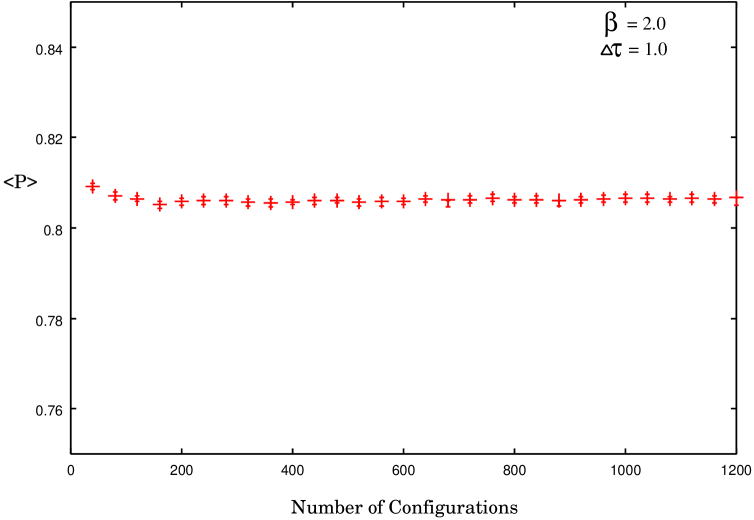
Figure 1: Plot of the mean plaquette value against the number of configurations.

After discarding the initial sweeps, the configurations were stored every 250 sweeps thereafter for later analysis. Ensembles of about 1,000 configurations were stored to measure the static quark potential and glueball masses at each $\beta$ for $\Delta\tau\geq 0.4$, and 1,400 configurations for $\Delta\tau\leq 0.333$. Measurements made on these stored configurations were grouped into 5 blocks, and then the mean and standard deviation of the final quantities were estimated by averaging over the ‘block averages’, treated as independent measurements. Each block average thus comprised 50,000 - 70,000 sweeps.

III.2 Interquark Potential

The static quark-antiquark potential, $V(\bf{r})$ for various spatial separations $\bf{r}$ is extracted from the expectation values of the Wilson loops. The timelike Wilson loops are expected to behave as:

$$W({\bf r},\tau)\simeq Z({\bf r})\mbox{exp}\big{[}-\tau V({\bf r})]+\mbox{(excited state contributions)}$$ (15)

We have averaged only over loops $({\bf x_{0}},\tau_{0})\rightarrow({\bf x_{0}+r},\tau_{0})\rightarrow({\bf x_{0}+r},\tau_{0}+\tau)\rightarrow({\bf x_{0}},\tau_{0}+\tau)\rightarrow({\bf x_{0}},\tau_{0})$ which follow either two sides of a rectangle between ${\bf x_{0}}$ and ${\bf x_{0}+r}$ or a single-step ‘staircase’ route, to estimate $W({\bf r},\tau)$. To suppress the excited state contributions, a simple APE smearing techniquealb87 ; tep86 was used on the space-like variables. In this technique an iterative smearing procedure is used to construct Wilson loop (and glueball) operators with a very high degree of overlap with the lowest-lying state. In our single-link smoothing procedure, we replace every space-like link variable by

$$U_{i}\rightarrow P\left[\alpha U_{i}+\frac{(1-\alpha)}{2}\sum_{s}U_{s}\right]$$ (16)

where the sum over “s” refers to the “staples”, or 3-link paths bracketing the given link on either side in the spatial plane, and P denotes a projection onto the group U(1), achieved by renormalizing the magnitude to unity. We used a smearing parameter $\alpha=0.7$ and up to ten iterations of the smearing process.

To further reduce the statistical errors, the timelike Wilson loops were constructed from “thermally averaged” temporal linkspar83 . That is, the temporal links $U_{t}$ in each Wilson loop were replaced by their thermal averages

$$\bar{U_{t}}=\int dUU\exp(-S[U])/\int dU\exp(-S[U])$$ (17)

where the integration is done over the one link only, and depends on the neighbouring links. For the U(1) model, the result can easily be computed in terms of Bessel functions involving the ‘staples’ adjacent to the link in question. This was done for all temporal links except those adjacent to the spatial legs of the loop, which are not ‘independent’par83 . The procedure has a dramatic effect in reducing the statistical noise, by up to an order of magnitudemor97 , worth a factor of 100 in Monte Carlo runtime.

The Wilson loop values $W({\bf r},\tau)$ are expected to decrease exponentially with Euclidean time $\tau$. A typical plot of the logrithmic ratios of successive loop values is shown in Figure 2 for $\beta=2.0$, $\Delta\tau=1.0$ and $R=\|{\bf r}\|=4$. It can be seen that with the heavy smearing we have used, a flat ‘plateau’ is attained virtually straight away. The Wilson loops are therefore fitted with the simple form

$$W({\bf r},\tau)=a\mbox{e}^{-\tau V(\bf r)}$$ (18)

to determine the ‘effective’ potential $V(\bf r)$.

Figure 2: Logarithmic ratio of Wilson loops as a function of $\tau$ for fixed $R=4$ at $\beta=2.0$ and $\Delta\tau=1.0$. The dashed horizontal line indicates the plateau value.

III.3 Glueball masses

Estimates for the glueball masses were obtained from the time-like correlations between spatial Wilson loop operators $\Phi_{i}(\tau))$,

$$C(\tau)=\langle\Phi_{i}(\tau)^{\dagger}\Phi_{i}(\tau)\rangle$$ (19)

in a standard fashion. As the temporal separation becomes large, the above correlator tends to be dominated by the lowest energy state carrying the quantum numbers of $\Phi$. If these quantum numbers coincide with those of the vacuum state, one then looks at the next higher energy state. So before taking the large Euclidean time limit, one subtracts the vacuum contribution from the correlator. Thus

$$\bar{\Phi}_{i}(\tau)=\Phi_{i}(\tau)-<0|\Phi_{i}(\tau)|0>$$ (20)

is a gauge invariant, translationally invariant, vacuum-subtracted operator capable of creating a glueball out of the vacuum. As a function of the temporal separation $\tau$, and with periodic boundary conditions, the correlation function is expected to behave as

$$C(\tau) = <\bar{\Phi}^{\dagger}_{i}(\tau)\bar{\Phi}_{i}(0)>$$ (21)

$$\simeq c_{1}(\exp(-m_{i}(\tau))+\exp(-m_{i}(T-\tau)))$$

$$+\mbox{(excited state contributions)}$$

where $m_{i}$ is the mass of the lowest glueball state in that sector, and $T=N_{\tau}a_{t}$ is the extent of the periodic lattice in the time direction. We project out states with momentum ${\bf k}=0$ and spin $J=0$ by summing over all lattice translations and rotations of the operators involved in $\Phi_{i}$. In the present case, we study only the lowest-lying ‘antisymmetric’ (PC = - -) and ‘symmetric’ (PC = ++) glueball states, corresponding to operators $\Phi_{i}$ which are the sine and cosine, respectively, of the sum of the link angles around the Wilson loop in question.

The statistical fluctuations in $C(\tau)$ are given bybra90

$$\sigma\rightarrow\frac{C(0)}{\sqrt{N}}$$ (22)

Thus, the signal-to-noise ratio collapses as $C(\tau)$ falls exponentially fast with $\tau$. Hence, it becomes important to use a glueball operator for which the overlap with the glueball state of interest is strong for small lattice spacing, and such that $C(\tau)$ attains its asymptotic form as quickly as possible. For such an operator, the signal-to-noise ratio is also optimalbra90 . Such operators can be constructed by exploiting link smearing and variational techniquesmor97 ; tep99 .

In the strong coupling limit $\beta=0$, the plaquette operator $U_{P}$ will create a symmetric glueball state from the vacuum. For large $\beta$, however, the glueball wave functions are expected to spread out and become more diffuse. To obtain a good overlap with the ground state in each sector at weak coupling, we need large, smooth operators $\phi_{i}$ on the lattice scale. An optimized operator is found by a variational technique, following Morningstar and Peardonmor97 and Tepertep99 . First, we calculate the correlation functions for square $n\times n$ Wilson loops with $m$ smearings, and determine the values of $m$ and $n$ for which the ratio $(C(1)/C(0))_{nm}$ is a maximum. In the second pass, an optimized glueball operator was found as a linear combination of the basic operators $\phi_{i}$,

$$\Phi(\tau)=\sum_{\alpha}v_{i\alpha}\phi_{i\alpha}(\tau)$$ (23)

where the index $\alpha$ runs over the rectangular Wilson loops with dimensions $l_{x}=[n-1,n+1]$, $l_{y}=[n-1,n+1]$ and smearings $n_{s}=[m-1,m+1]$ with $n$ and $m$ as determined in the first pass, making 27 operators in all. The $27\times 27$ correlation matrix was computed

$$C_{i\alpha\beta}(\tau)=\sum_{\tau 0}<0|\bar{\phi}_{i\alpha}(\tau+\tau_{0})\bar{\phi}_{i\beta}(\tau_{0})|>$$ (24)

where $\bar{\phi}_{i\alpha}(\tau)$ is a vacuum-subtracted operator

$$\bar{\phi}_{i\alpha}(\tau)=\phi_{i\alpha}(\tau)-<0|\phi_{i\alpha}(\tau)|0>$$

The coefficients $v_{i\alpha}$ were then determined by minimizing the effective mass at $\tau=1$

$$\tilde{m}(1)=-\frac{1}{a_{t}}\ln\left[\frac{\sum_{\alpha\beta}v_{i\alpha}v_{i\beta}C_{i\alpha\beta}(1)}{\sum_{\alpha\beta}v_{i\alpha}v_{i\beta}C_{i\alpha\beta}(0)}\right]$$ (25)

Let ${\bf{v}}_{i}$ denote a column vector whose elements are the optimal values of the coefficients $v_{i\alpha}$, then the column vector ${\bf{v}}_{i}$ formed from the $v_{i\alpha}$ is the solution of an eigenvalue equation

$$C(1){\bf{v}}_{i}=\mbox{e}^{-a_{t}\tilde{m}(1)}C(0){\bf{v}}_{i}$$ (26)

The eigenvector ${\bf{v}}_{0}$ corresponding to the largest eigenvalue $\mbox{e}^{-a_{t}\tilde{m}}$ then yields the coefficients for the operator $\Phi_{i}(\tau)$ which best overlaps the lowest-lying state.

A third pass was made to estimate the optimized correlation function

$$C_{i}(\tau)=\sum_{\tau_{0}}<0|\bar{\Phi}_{i}(\tau+\tau_{0})\bar{\Phi}_{i}(\tau_{0})|0>$$ (27)

Finally the optimized correlation function was fitted with the simple form

$$C_{i}(\tau)=c_{1}\cosh m_{i}(\frac{T}{2}-\tau)$$ (28)

to determine the glueball mass estimates. Figure 3 shows an example of the correlation function and fit for the antisymmetric state at $\beta=2$ and $\Delta\tau=1$. It can be seen that the form (28) fits the data very well.

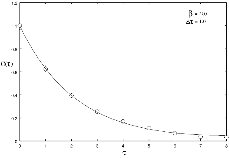
Figure 3: Antisymmetric glueball correlation function $C(\tau)$ for the $0^{--}$ channel against $\tau$ at $\Delta\tau=1.0$ and $\beta=2.0$. The solid curve is a fit to the simulation results using Eq. (28).

IV Simulation results at finite lattice size

Simulations were carried out for lattices of $N_{s}^{2}\times N_{t}$ sites, with $N_{s}=16$ and $N_{t}$ ranging from 16 to 48 sites, with periodic boundary conditions. Each run involved 250,000 sweeps (350,000 for high anisotropy) of the lattice, with 50,000 sweeps (100,000 high anisotropy) discarded to allow for equilibrum, and configurations recorded every 250 sweeps thereafter. Coupling values from $\beta=1.0$ to 3.0 were explored at anisotropies $\Delta\tau$ ranging from 1 to 1/3. We fixed $\Delta\tau=16/N_{t}$ in the first pass, so that the lattice size remains fixed at $16a_{s}$ in all directions. At strong couplings (small $\beta$), we expect the behaviour to be the same as in the bulk system, but at weaker couplings (large $\beta$) the finite-size/finite-temperature corrections will become more important. We shall monitor our data for signs of these effects. The results for the Euclidean case $\Delta\tau=1$ are listed in Table 1.

Table 1: Monte Carlo estimates for the mean plaquette $<P>$, string tension $K$, symmetric and antisymmetric glueball masses $M_{0^{++}}$, $M_{0^{--}}$, and the mass ratio $R_{M}$ in the Euclidean case $\Delta\tau=1.0$.

$\beta$	$<P>$	K	$M_{0^{++}}$	$M_{0^{--}}$	$R_{M}$
1.0	0.475	0.674	2.69(1)	2.6(1)	1.00(6)
1.35	0.629	0.343(6)	2.14(5)	1.65(5)	1.29(5)
1.41	0.656	0.286(5)	2.08(5)	1.58(3)	1.31(7)
1.55	0.704	0.200(1)	1.79(5)	1.26(3)	1.41(7)
1.70	0.748	0.122	1.41(3)	0.88(1)	1.60(8)
1.90	0.790	0.082	1.14(3)	0.54(1)	2.0(1)
2.0	0.806	0.050	0.79(1)	0.44(1)	1.78(9)
2.25	0.834	0.022	0.50(2)	0.236(9)	2.1(1)
2.5	0.854	0.012	0.34(2)	0.165(9)	2.0(1)
2.75	0.869	0.009
3.0	0.881	0.010

IV.1 Mean Plaquette

Figure 4 shows the behaviour of the mean spatial plaquette $<P>$ for different $\beta$, at fixed $\Delta\tau=1$ (Euclidean, isotropic case). A strong coupling perturbation series expansion has been obtained for this quantity by Bhanot and Creutzbha80 to order $\beta$, and a weak coupling series to order $1/\beta^{5}$ by Horsley and Wolffhor81 . These series are represented by solid and dashed lines on the graph, respectively. It can be seen that the data follow the strong-coupling expansion for $\beta\leq 1.5$, and match the weak-coupling expansion quite closely beyond $\beta\simeq 2$. The variation of $<P>$ with coupling is extremely smooth, with no sign of any phase transition, as we should expect. The cross-over from strong to weak coupling seems to take place quite rapidly in the region $\beta\approx 1.8-2.0$. Horsley and Wolff hor81 investigated the effect of a finite-size lattice in their weak-coupling expansion calculations. They found that such effects enter at order $1/\beta^{2}$ as a correction of order $1/L^{D}$, where $L$ is the lattice size and $D$ is the number of dimensions. Thus for the compact U(1) model in 3-dimensions and $L>10$, the finite size effects should be essentially negligible.

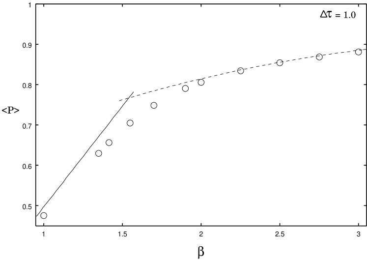
Figure 4: The mean plaquette as a function of $\beta$ at $\Delta\tau=1$. The circles are our Monte Carlo estimates. The solid curve represents the $O(\beta)$ strong-coupling expansion bha80 and the dashed curve represents the $O(1/\beta^{4})$ weak-coupling expansion hor81 .

Figure 5 shows a plot of our estimates of $<P>$ as a function of anisotropy irv84 ${\Delta\tau}^{2}$ for the case $\beta=\sqrt{2}$. It can be seen that $<P>$ remains almost constant. We would like to make contact with previous Hamiltonian studies by showing that the mean plaquette value approaches to previously known values in the Hamiltonian limit $\Delta\tau\rightarrow 0$. The extrapolation was performed using a simple cubic fit in powers of $\Delta\tau^{2}$. In this limit our results agree very well with the Hamiltonian estimate obtained by Hamer et alham00 . Our general estimates in the Hamiltonian limit $\Delta\tau=0$ are listed in Table 2.

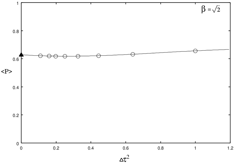
Figure 5: The mean plaquette as a function of $\Delta\tau^{2}$ at $\beta=\sqrt{2}$. The solid curve is a cubic fit to the data, extrapolated to the Hamiltonian limit. The triangle shows the Hamiltonian series estimate ham00 in that limit.

Table 2: Monte Carlo estimates for the mean plaquette $<P>$, string tension $K$, symmetric and antisymmetric glueball masses $M_{0^{++}}$, $M_{0^{--}}$, and the mass ratio $R_{M}$ in the Hamiltonian limit $\Delta\tau=0$.

$\beta$	$<P>$	K	$M_{0^{++}}$	$M_{0^{--}}$	$R_{M}$
1.0	0.397(6)	0.302(3)	1.9(1)	1.45(7)	1.32(1)
1.35	0.599(2)	0.132(8)	1.4(1)	0.9(1)	1.5(2)
1.41	0.628(1)	0.104(7)	1.05(6)	0.60(7)	1.7(2)
1.55	0.651(1)	0.085(9)	0.8(2)	0.3(1)	2.1(1.1)
1.70	0.695(3)	0.021(6)	0.5(3)	0.24(9)	2.2(1.5)
1.90	0.716(4)	0.018(7)	0.3(1)	0.17(9)	2.2(1.5)
2.0	0.740(4)	0.015(1)	0.2(1)	0.10(6)
2.25	0.779(4)	0.008(4)	0.15(9)	0.07(5)
2.5	0.796(5)	0.005(8)
2.75	0.820(5)
3.0	0.839(4)

Figure 6 graphs the resulting estimates of $<P>$ in the Hamiltonian limit $\Delta\tau=0$ as a function of coupling $\beta$. The weak-couplingham93 and strong-couplingham92 series predictions are shown as dashed and solid lines on the graph respectively, while some previous Greens Function Monte Carlo estimates ham00 are shown as triangles. Our present results are generally in reasonable agreement with the earlier ones, if perhaps a little low in places. It can be seen that the crossover from strong to weak coupling behaviour again occurs at around $\beta\simeq 1.8$.

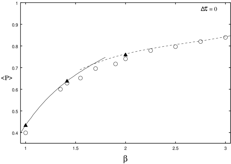
Figure 6: Mean plaquette estimates as a function of $\beta$ at $\Delta\tau=0$. Our present Monte Carlo estimates are shown by circles. The strong-coupling ham92 and weak-coupling ham93 series predictions are shown as solid and dashed lines respectively. The GFMC estimates ham00 are represented by the solid triangles.

IV.2 Static quark potential and string tension

Figure 7 shows a graph of the static quark potential V(R) as a function of radius R at $\beta=2.0$ and $\Delta\tau=1.0$. To extract the string tension, the curve is fitted by a form

$$V(R)=a+b\ln R+\sigma R,$$ (29)

including a logarithmic Coulomb term as expected for classical QED in (2+1) dimensions which dominates the behaviour at small distances, and a linear term as predicted by Polyakovpol78 and Göpfert and Mackgop82 dominating the behaviour at large distances. The linear behaviour at large distances is very clear, but the data do not extend to very small distances, so there is no real test of the presumed logarithmic behaviour in this regime.

Figure 7: The static-quark potential $V(R)$ as a function of the separation R. This plot involves measurements at $\beta=2.0$ for $\Delta\tau=1.0$ with 10 smearing sweeps at smearing parameter $\alpha=0.7$. The errors are smaller than the symbols. The dashed line is a fit to the form $V(R)=a+bR+c\mbox{ln}(R)$.

Figure 8 shows the behaviour of the fitted value of the string tension $K=\sigma a^{2}$ as a function of $\beta$ for the Euclidean, isotropic case ($\Delta\tau=1$). The solid line on the graph represents the form (6) predicted by Göpfert and Mackgop82 , using a value of $c=44.0\pm 0.4$. It can be seen that this form represents the data rather well over a range $1.41\leq\beta\leq 2.5$; in fact an unconstrainted fit to the data gives a slope of $2.49\pm 0.15$, extremely close to the predicted value 2.494. The coefficient $c$, however, is much bigger than the value $c=8$ predicted in the classical approximation. It would be interesting to explore how higher-order quantum corrections affect the prediction for $c$.

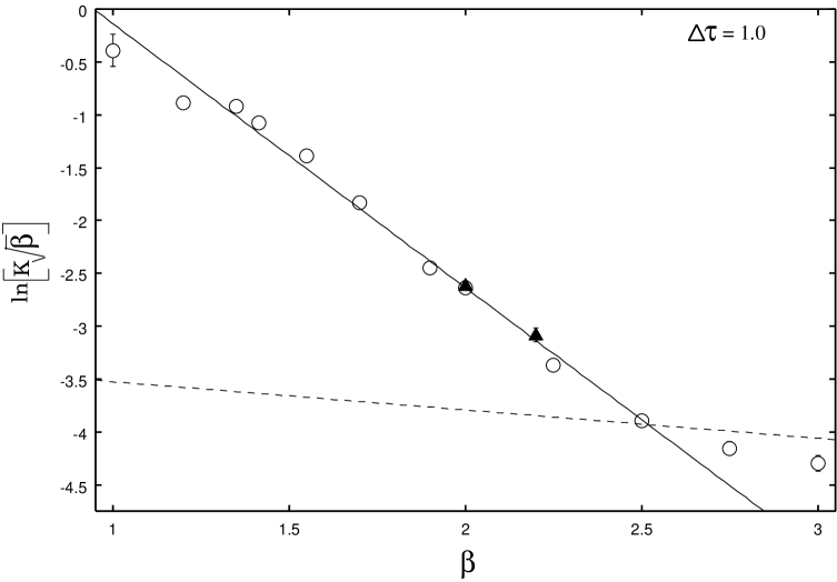
Figure 8: $\mbox{ln}(K\sqrt{\beta})$ as a function of $\beta$ at $\Delta\tau=1.0$. The solid curve represents the predicted asymptotic form, eq. (6), with our estimated value for the normalization constant, $c=44.0\pm 0.4$. The dashed line represents the finite size scaling behaviourham93 . The solid triangles show the previous estimates of Irbäck and Peterson irb87 .

The dashed line in Figure 8 gives some idea of the expected finite-size scaling corrections to the string tension. These have not been calculated explicitly for the Euclidean model, as far as we are aware, but in the Hamiltonian version the string tension at weak coupling is foundham93 to behave as

$$K=\frac{1}{2\beta L}$$ (30)

where $L=N_{s}$ is the lattice size (here $L=16$), and this is represented by the dashed line. This would predict that the string tension will be dominated by finite-size corrections beyond $\beta\simeq 2.5$, and indeed the Monte Carlo estimates do flatten out beyond that point, although at a level below equation (30).

Figure 9 shows the behaviour of the string tension $K$ as a function of the anisotropy ${\Delta\tau}^{2}$, for fixed coupling $\beta=\sqrt{2}$. An extrapolation to the Hamiltonian limit $\Delta\tau\rightarrow 0$ is performed by a simple cubic fit. Again the extrapolation agrees well with earlier Hamiltonian estimatesham94 . Note that this quantity depends rather strongly on $\Delta\tau$: there is a factor of three difference between the values at $\Delta\tau=0$ and $\Delta\tau=1$. Extrapolating to $\Delta\tau\rightarrow 0$, estimates of the string tension in the Hamiltonian limit are obtained for various $\beta$ values.

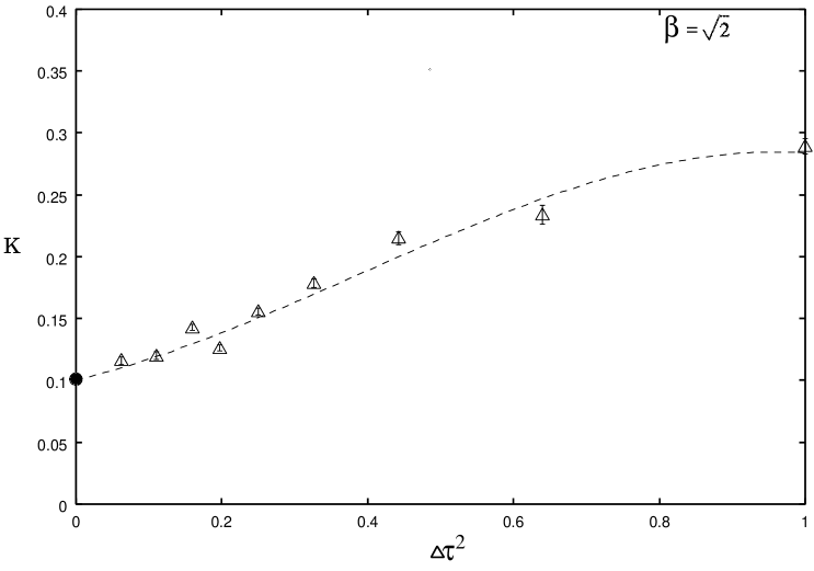
Figure 9: String tension, K, as a function of $\Delta\tau^{2}$ at $\beta=\sqrt{2}$. An extrapolation to the Hamiltonian limit is performed by a cubic fit and shown by the dashed line. Our MC estimates are shown by triangles and an earlier Hamiltonian series estimate ham92 is shown by a solid circle.

Our estimates of the string tension in the Hamiltonian limit are graphed in Figure 10, together with earlier results from an ‘exact linked cluster expansion’irv84 and a quantum Monte Carlo simulationham94 . It can be seen that our values are consistent with earlier results, though less accurate, and extend further into the weak-coupling region. The solid line in the graph represents a least-square fit of the weak-coupling asymptotic form (6), with $v(0)=0.3214$ and $c=46.7\pm 0.4$. This form represents the data well for $1.35\leq\beta\leq 2.0$. Beyond $\beta=2$ the string tension is consistent, within errors, with the finite-size behaviour predicted by equation (30), which is shown as a dashed line.

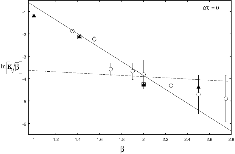
Figure 10: Graph showing estimates of the string tension in the Hamiltonian limit as a function of $\beta$. The solid line is a least square fit to the form $K=\beta^{-1/2}\mbox{exp}(a_{0}-a_{1}\beta)$, with $a_{0}=2.359$ and $a_{1}=3.159$. The dashed line represents the finite size scaling behaviourham93 . Earlier results from an exact linked cluster expansionirv84 and quantum Monte Carlo simulations ham94 are shown as solid triangles and squares respectively.

IV.3 Glueball Masses

Figure 11 shows results for the antisymmetric $0^{--}$ glueball mass against $\beta$ for the isotropic Euclidean case $\Delta\tau=1$. The solid line on the graph is a fit to the data over the range $1.4\leq\beta\leq 2.25$ using the predicted asymptotic form, equation (5), but with an additional multiplying constant:

$$M=am_{D}=c_{1}\sqrt{8\pi^{2}\beta}\exp(-\pi^{2}\beta v(0))$$ (31)

where $c_{1}=5.23\pm 0.11$ when adjusted to fit the data. Thus the slope, $2.48\pm 0.09$, of the data matches the predicted asymptotic form very nicely, but the coefficient is too large by a factor of $5.2$. It would again be interesting to explore whether this discrepancy could be due to quantum corrections.

The expected finite-size scaling behaviour of the mass gap near the continuum critical point in this model is not known; but Weigel and Jankewei99 have performed a Monte Carlo simulation for an O(2) spin model in three dimensions which should lie in the same universality class, obtaining

$$M\sim 1.3218/L$$ (32)

for the magnetic gap. The dashed line in Figure 11 shows this prediction for $L=16$. It can be seen that the Euclidean mass gap should not be affected by finite-size corrections until $\beta\geq 2.8$.

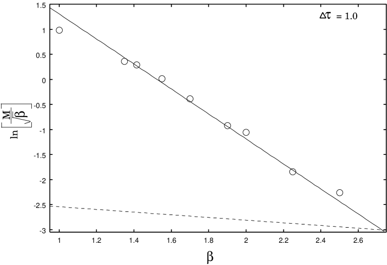
Figure 11: The scaling behaviour of the antisymmetric mass gap against $\beta$ at $\Delta\tau=1.0$. The solid line is a fit of the form eq. (31). The errors are smaller than the symbols. The dashed line shows the finite size scaling behaviour wei99 .

To check the consistency of our method, we plot the dimensionless ratio of the antisymmetric mass gap over the square root of the string tension against $\beta$ together with the results of Tepertep99 in Figure 12. The agreement is excellent. The solid line gives the ratio of the fits in Figures 8 and 11, and shows how this ratio vanishes exponentially in the weak-coupling limit, whereas in four-dimensional confining theories it goes to a constant.

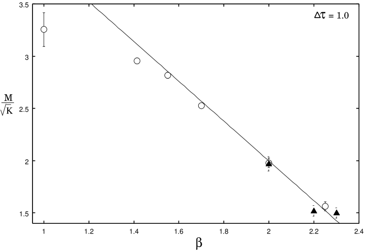
Figure 12: The dimensionless ratio $M/\sqrt{K}$ as a function $\beta$. Our estimates are shown by circles and solid triangles show the earlier results of Teper tep99 . The solid curve represents the predicted weak-coupling behaviour.

Figure 13 shows the behaviour of the glueball masses as functions of ${\Delta\tau}^{2}$ for $\beta=\sqrt{2}$. The extrapolation to the Hamiltonian limit is performed by a simple cubic fit in powers of $\Delta\tau^{2}$. In this limit we reproduce the earlier estimates of Hamer et alham92 for the $0^{--}$ and $0^{++}$ states.

Estimates of the antisymmetric mass gap in the Hamiltonian limit $\Delta\tau=0$ are graphed against $\beta$ in Figure 14. Also shown are results from previous strong-coupling series extrapolationsham92 and quantum Monte Carlo calculationsham94 . It can be seen that our present results agree with previous estimates but are less accurate. The solid line is a fit to our data for $1.4\leq\beta\leq 2.25$ of the form (28), with $v(0)=0.3214$ and $c_{1}=5.5\pm 0.2$, which is similar to the coefficient found in the Euclidean case. The fit to the data gives a slope of $3.1\pm 0.2$ and an intercept of $3.6\pm 0.3$ of the scaling curve. We note that the exponential slope in previous studies is generally somewhat less than this, as tabled in john97 and as illustrated by the black triangles in Figure 14. The dashed line represents the finite-size scaling behaviour, equation (32), which we assume holds in the Hamiltonian limit also, for want of better information. It can be seen that the finite-size corrections are predicted to dominate for $\beta\geq 2.2$, but the date are not accurate enough at weak couplings to establish whether this is really the case.

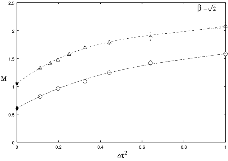
Figure 13: Estimates of the masses of $0^{++}$ and $0^{--}$ glueballs against $\Delta\tau^{2}$. Results at $\beta=\sqrt{2}$ for the $0^{++}$ and $0^{--}$ are labeled by circles and triangle respectively. The solid and dashed curves are the cubic fits to the data extrapolated to the Hamiltonian limit. The series estimates of Hamer et al ham92 in the limit $\Delta\tau\rightarrow 0$, for symmetric and antisymmetric channels are shown as a star and diamond respectively.

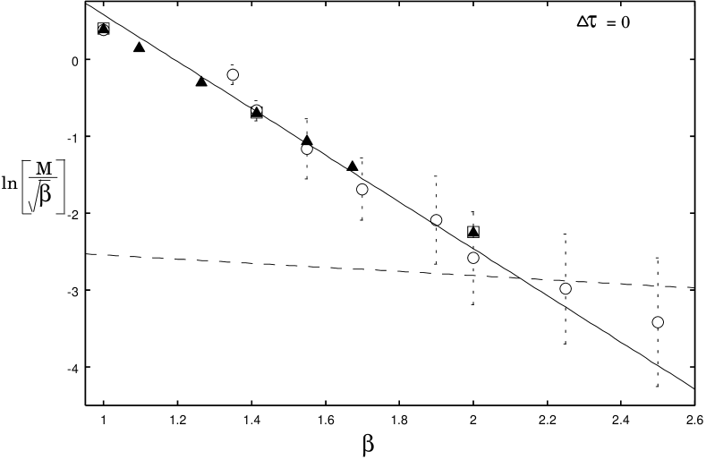
Figure 14: Hamiltonian estimates of the antisymmetric mass gap plotted as a function of $\beta$. The solid curve is the fit to the data for $1.4<\beta<2.25$. The dashed line represents the finite size effects wei99 . The previous results from series expansion ham92 and quantum Monte Carlo calculations ham94 are shown as solid triangles and open squares respectively.

Finally, Figure 15 displays the behaviour of the dimensionless mass ratio,

$$R_{M}=M(0^{++})/M(0^{--})$$ (33)

for the Euclidean case $\Delta\tau=1$. As in the (3+1)D confining theories, we may expect that quantities of this sort will approach their weak-coupling or continuum limits with corrections of $O(1/a_{eff})$, where $a_{eff}$ is the effective lattice spacing in ‘physical’ units when the mass gap has been renormalized to a constant. Hence for our present purposes we define $a_{eff}$ from equation (5) as

$$a_{eff}=\sqrt{8\pi^{2}\beta}\exp(-\pi^{2}\beta v(0))$$ (34)

with $v(0)=0.2527$ for the Euclidean case. The mass ratio is plotted against $a_{eff}$ in Figure 15. At weak coupling, we expect the theory to approach a theory of free bosonsgop82 so that the symmetric state will be composed of two $0^{--}$ bosons and the mass ratio should approach two. Our results show that as $a_{eff}$ goes to zero, the mass ratio rises to around the expected value of $2.0$. A linear fit to the data from $0.08\leq a_{eff}\leq 0.32$ gives an intercept $R_{M}=1.95\pm 0.05$. However, we note that the last two of our estimates, together with two from Tepertep99 , lie considerably above $R_{M}=2$. In the bulk system, of course, the ratio cannot rise above 2, because it is always possible to construct a $0^{++}$ state out of two $0^{--}$ mesons. These points correspond to couplings $\beta>2$, and we conjecture that they may be affected by finite-size corrections: a simulation on a larger lattice would be necessary to check on this point. Our last two points have not been included in the fit.

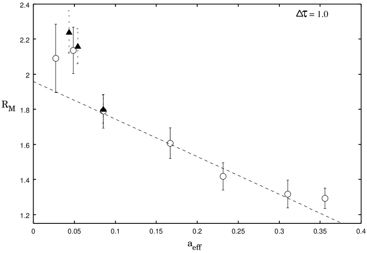
Figure 15: A graph showing estimates of the mass ratio $R_{M}$ as a function of the effective spacing, $a_{eff}$, at $\Delta\tau=1.0$. Our present estimates are shown by the circles. The dashed line is a linear fit to the data over the range $0.08\leq a_{eff}\leq 0.31$. The solid triangles show the previous estimates of Teper tep99 .

Figure 16: Mass ratio in the Hamiltonian limit as a function of the effective spacing, $a_{eff}$, at $\Delta\tau=0$. Our MC estimates are shown by the circles. Earlier series ham92 and quantum Monte Carlo ham00a results are shown by solid triangles and open squares respectively. The dashed line is a linear fit to the earlier data from series expansions ham92 over the range $0.02\leq a_{eff}\leq 0.12$.

Figure 16 shows a similar graph for the Hamiltonian limit, $\Delta\tau=0$. Within errors, our present results are consistent with earlier seriesham92 and quantum Monte Carloham94 estimates, but are much less accurate, and tend to lie consistently on the high side. A linear fit to the earlier data from $0.02\leq a_{eff}\leq 0.12$ gives $R_{M}=2.14\pm 0.01$.

V Conclusions

In this paper, we have applied standard Euclidean path integral Monte Carlo methods to the U(1) model in (2+1) dimensions on an anisotropic lattice, and taken the anisotropic limit $\Delta\tau\rightarrow 0$ to obtain the Hamiltonian limit of the model.

We have obtained the first clear picture of the static quark potential in this model, showing very clear evidence of the linear confining behaviour at large distances predicted by Polyakovpol78 . There is also a turnover at short distances consistent with a logarithmic Coulomb behaviour in that regime.

In the isotropic or Euclidean case $\Delta\tau=1$, the string tension and mass gap display an exponential decrease at weak couplings which is in excellent agreement with the behaviour predicted by Polyakovpol78 and Göpfert and Mackgop82 . Both quantities, however, are 5-6 times larger in magnitude than the theory predicts. It would be interesting to calculate whether higher-order quantum corrections can account for this discrepancy.

The dimensionless ratio $M/\sqrt{K}$ scales exponentially to zero in the weak-coupling or continuum limit, as predicted by the theory. The mass ratio of the two lowest glueball states scales against the effective lattice spacing towards a value close to $2.0$, as expected for a theory of free scalar bosons, apart from some anomalous results at large $\beta$ which we have ascribed to finite-lattice effects.

In the anisotropic or Hamiltonian limit $\Delta\tau\rightarrow 0$, our results are less accurate, because of the extrapolation needed to reach this limit. Nevertheless, the results are generally in good agreement with those obtained by other methods. Once again, an exponential behaviour of the string tension and glueball masses can be demonstrated at weak coupling. The dimensionless mass ratio again scales to a value near $2.0$. Because the exponential slope is steeper, finite-size effects seem to be somewhat more important in the Hamiltonian regime than in the Euclidean one.

Our major object in this study was to compare the Euclidean PIMC approach to quantum Monte Carlo methods such as Green’s Function Monte Carlo (GFMC) for obtaining estimates in the Hamiltonian limit. The PIMC approach suffers from the disadvantage that an extrapolation is necessary to reach the limit $\Delta\tau\rightarrow 0$; while GFMC suffers from the major disadvantage that it relies on a ‘trial wave function’. In the event, we have obtained much better results using PIMC. A clear and consistent picture of the string tension and glueball masses was obtained at weak coupling. Using GFMC, on the other hand, only qualitative estimates of the string tension were obtained, and the glueball mass estimates were virtually worthlessham00 . No doubt there are many ‘tricks of the trade’, such as smearing and variational techniques, which could be used to improve the GFMC results; but we found previouslyham00a that there is an unacceptably strong dependence on the trial wave function using that technique, especially for large lattice size. The PIMC technique seems to offer a much more robust and unbiased approach to Hamiltonian lattice gauge theories. Of course, one must generally expect the Hamiltonian estimates to be less accurate than the Euclidean ones because of the extra extrapolation involved.

We note that the PIMC results are still less accurate than some older quantum Monte Carlo results of Hamer, Wang and Priceham94 . The latter were obtained using a strong-coupling representation, however, and this approach has been found to fail for non-Abelian modelsham94 due to the occurrence of a ‘minus sign’ problem, as mentioned in the introduction.

- (1) M. Creutz, Phys. Rev. Letts. 43, 553 (1979)
- (2) K.G. Wilson, Phys. Rev. D10, 2445 (1974)
- (3) J. Kogut and L. Susskind, Phys. Rev. D11, 395 (1975)
- (4) C.J. Morningstar and M. Peardon, Phys. Rev. D56, 4043 (1997)
- (5) C. J. Hamer, M. Sheppeard, W. H. Zheng and D. Schütte, Phys. Rev. D54, 2395 (1996)
- (6) T.Banks, S. Raby, L. Susskind, J. Kogut, D.R.T. Jones, P.N. Scharbach and D.K. Sinclair, Phys. Rev. D15, 1111 (1977)
- (7) D. Horn and M. Weinstein, Phys. Rev. D30, 1256 (1984)
- (8) Guo Shuohong, Zheng Weihong and Liu Jiunmin, Phys. Rev. D38, 2591 (1988)
- (9) J. McIntosh and L. Hollenberg, Z. Phys. C76, 175 (1997)
- (10) J.M. Aroca and H. Fort, Phys. Letts. B317, 604 (1993)
- (11) T.M.R. Byrnes, P.Sriganesh, R.J. Bursill and C.J. Hamer, to be published in Phys. Rev. D
- (12) D.Blankenbecler and R.L. Sugar, Phys. Rev. D27, 1304( 1983)
- (13) T.A. DeGrand and J. Potvin, Phys. Rev. D31, 871 (1985)
- (14) C. J. Hamer, K. C. Wang and P. F. Price, Phys. Rev. D50, 4693 (1994)
- (15) S. A. Chin, J. W. Negele and S. E. Koonin, Ann. Phys. (N.Y.) 157, 140 (1984)
- (16) D. W. Heys and D. R. Stump, Phys. Rev. D28, 2067 (1983)
- (17) Kalos M. H., J. Comp. Phys. 1, 257 (1966); D. M. Ceperley and M. H. Kalos, in Monte Carlo Methods in Statistical Mechanics, ed. K. Binder (Springer-Verlag, New York, 1979).
- (18) M. Samaras and C. J. Hamer, Aust. J. Phys. 52, 637 (1999)
- (19) C.J. Hamer, R.J. Bursill and M. Samaras, Phys. Rev. D62, 054511 (2000)
- (20) C.J. Hamer, R.J. Bursill and M. Samaras, Phys. Rev. D62, 074506 (2000)
- (21) K.S. Liu, M.H. Kalos and G.V. Chester, Phys. Rev. A10 303 (1974)
- (22) P. A. Whitlock, D. M. Ceperley, G. V. Chester and M. H. Kalos, Phys. Rev. B19, 5598 (1979)
- (23) J. Ambjorn, A.J.G. Hey and S. Otto, Nucl. Phys. B210, 347 (1982)
- (24) P.D. Coddington, A.J.G. Hey, A.A. Middleton and J.S. Townsend, Phys. Letts. B175, 64 (1986)
- (25) A. Irbäck and C. Peterson, Phys. Rev. D36, 3804 (1987)
- (26) L. Gross, Commun. Math. Phys. 92, 137 (1983)
- (27) A.M. Polyakov, Phys. Lett. 72B, 477 (1978)
- (28) M. Göpfert and G. Mack, Commun. Math. Phys. 82, 545 (1982)
- (29) T. Banks, R. Myerson and J. Kogut, Nucl. Phys. B129, 493 (1977).
- (30) S. Ben-Menahem, Phys. Rev. bf D20, 1923 (1979).
- (31) C. J. Hamer, J. Oitmaa, and Zheng Weihong, Phys. Rev. D45, 4652 (1992)
- (32) C.J.Hamer, Zheng Weihong and J. Oitmaa, Phys. Rev. D53, 1429 (1996)
- (33) A.C. Irving, J.F. Owens and C.J.Hamer, Phys. Rev. D28, 2059 (1983)
- (34) D. Horn, G. Lana and D. Schreiber, Phys. Rev. D36, 3218 (1987)
- (35) C.J. Morningstar, Phys. Rev. D46, 824 (1992)
- (36) A. Dabringhaus, M.L. Ristig and J.W. Clark, Phys. Rev. D43, 1978 (1991)
- (37) X.Y. Fang, J.M. Liu and S.H. Guo, Phys. Rev. D53, 1523 (1996)
- (38) S.J. Baker, R,.F. Bishop and N.J. Davidson, Phys. Rev. D53, 2610 (1996).
- (39) S. E. Koonin, E. A. Umland and M. R. Zirnbauer, Phys. Rev. D33, 1795 (1986)
- (40) C. M. Yung, C. R. Allton and C. J. Hamer, Phys. Rev. D33, 1795 (1986)
- (41) C. J. Hamer and Zheng Weihong, Phys. Rev. D48, 4435 (1993)
- (42) G.G. Batrouni, G.R. Katz, A.S. Kronfeld, G.P. Lepage, B.Svetitsky and K.G. Wilson, Phys. Rev. D32, 2736 (1985)
- (43) C.T.H. Davies, G.G. Batrouni, G.R. Katz, A.S. Kronfeld, G.P. Lepage, P. Rossi, B. Svetitsky and K.G. Wilson, Phys. Rev. D41, 1953 (1990)
- (44) M. Albanese et al., Phys. Lett. B192, 163 (1987)
- (45) M. Teper, Phys. Lett. B183, 345 (1986); K.Ishikawa, A. Sato, G. Schierholz and M. Teper, Z. Phs. C21, 167 (1983)
- (46) G. Parisi, R. Petronzio and F. Rapuano, Phys. Lett. 128B, 418 (1983)
- (47) F. Brandstaeter et al., Nucl.Phys. B345, 709 (1990)
- (48) M.J. Teper, Phys. Rev. D59, 014512 (1999)
- (49) G. Bhanot and M. Creutz, Phys. Rev. D21, 2892 (1980)
- (50) R. Horsley and U. Wolff, Phys. Letts. B105, 290 (1981)
- (51) A.C. Irving and C.J. Hamer, Nucl. Phys. B235, 358 (1984)
- (52) M. Weigel and W. Janke, Phys. Rev. Letts. 82, 2318 (1999)