The radial distributions of a heavy-light meson on a lattice

Abstract

In an earlier work [1], the charge (vector) and matter (scalar) radial distributions of heavy-light mesons were measured in the quenched approximation on a $16^{3}\times 24$ lattice with $\beta=5.7$, a lattice spacing of $a\approx 0.17$ fm, and a hopping parameter corresponding to a light quark mass about that of the strange quark.

Several improvements are now made [2]:

1. The configurations are generated using dynamical fermions with quark-gluon coupling $\beta=5.2$ ($a\approx 0.14$ fm);

2. Many more gauge configurations are included (78 compared with the earlier 20);

3. The distributions at many off-axis, in addition to on-axis, points are measured;

4. The data analysis is much more complete. In particular, distributions involving excited states are extracted.

The exponential decay of the charge and matter distributions can be described by mesons of mass 0.9$\pm 0.1$ and 1.5$\pm 0.1$ GeV respectively — values that are consistent with those of vector and scalar $q\bar{q}$-states calculated directly with the same lattice parameters.

1 INTRODUCTION

A knowledge of the radial distributions of quarks inside hadrons could lead to a better understanding of the QCD description of these hadrons and possibly suggest forms for phenomenological models. As a step in this direction, we have measured the charge (vector) and matter (scalar) densities of a heavy-light meson.

More explicitly, the heavy-light meson is simplified to being an infinitely heavy quark ($Q$) and an antiquark ($\bar{q}$) with a mass approximately equal to that of the strange quark. The physical meson nearest to this idealised meson is the $B_{{\rm s}}$(5.37 GeV). We consider two flavours of dynamical quarks ($u$ and $d$).

2 MEASUREMENTS

2.1 Energies

The basic quantity for evaluating the energies of a heavy-light meson is the 2-point correlation function – see Fig. 1 a) –

$$C_{2}(T)=\langle U^{Q}(\mathbf{x},t,T)P(\mathbf{x},t+T,t)\rangle,$$ (1)

where $U^{Q}(\mathbf{x},t,T)$ is the heavy (infinite mass)-quark propagator and $P(\mathbf{x},t+T,t)$ the light anti-quark propagator. The $\langle...\rangle$ means the average over the whole lattice.

Figure 1: Two- and three-point correlation functions $C_{2}(T)$ and $C_{3,c(m)}(T,\mathbf{r})$.

2.2 Heavy-light radial correlations

When measuring the radial correlations, the basic quantity is the 3-point correlation function – see Fig. 1 b) –

$$C_{3,c(m)}(T,\mathbf{r})=\langle U^{Q}P_{1}\Theta P_{2}\rangle,$$ (2)

where the $P_{1,2}$ are the light anti-quark propagators that go from the $Q$ at time $t_{1}$ to the point $\mathbf{r}$ at $t=0$ and then return to $Q$ at time $-t_{2}$. Here $T=t_{1}+t_{2}$. The probe $\Theta$ at $\mathbf{r}$ is here considered to have two forms: i) $\Theta=\gamma_{4}$ for measuring the charge distribution (c) of the $\bar{q}$ and ii) $\Theta=1$ for measuring the matter distribution (m).

The strategy is to first fit the $\langle C_{2}(T)\rangle$ by the approximate expression

$$\tilde{C}_{2}(T)=\sum_{\alpha}v^{\alpha}\mathrm{e}^{-E_{\alpha}T}v^{\alpha}.$$ (3)

This results in the energy eigenvalues $E_{\alpha}$ and their eigenvectors $v^{\alpha}$ (Ref. [3]).

Given the $E_{\alpha}$ and $v^{\alpha}$, the $C_{3,c(m)}(T,\mathbf{r})$ are then fitted by

$$\tilde{C}_{3,c(m)}(T,\mathbf{r})=\sum_{\alpha\beta}v^{\alpha}\mathrm{e}^{-E_{\alpha}t_{1}}x^{\alpha\beta}(r)\mathrm{e}^{-E_{\beta}t_{2}}v^{\beta},$$ (4)

where the $x^{\alpha\beta}(r)$ are varied giving directly the desired charge or matter density. In this work two levels of fuzzing with 2 and 8 iterations were used in addition to the unfuzzed lattice. This enabled us to extract information of the excited states as well.

3 RESULTS

3.1 Fits to the charge and matter densities

It is convenient to parametrize the radial correlations in some simple way. We have considered pure exponential and Yukawa fits to the data as well as their lattice forms

$$\frac{\pi a}{2r^{\mathrm{E}}L^{3}}\sum_{\mathbf{q}}\frac{\cos(\mathbf{r}\cdot\mathbf{q})}{\bigl{[}\sum^{3}_{\begin{subarray}{c}i=1\end{subarray}}\sin^{2}(\frac{aq_{i}}{2})+(\frac{a}{2r^{\mathrm{E}}})^{2}\bigr{]}^{2}}$$ (5)

(lattice exponential) and

$$\frac{\pi}{aL^{3}}\sum_{\mathbf{q}}\frac{\cos(\mathbf{r}\cdot\mathbf{q})}{\sum^{3}_{i=1}\sin^{2}(\frac{aq_{i}}{2})+(\frac{a}{2r^{\mathrm{Y}}})^{2}}$$ (6)

(lattice Yukawa).

They all fit the data well, and the lattice forms are able to reproduce some of the structure (lattice artefacts) — see Fig. 2. The exponential decay of the charge and matter distributions can be described by mesons of mass $0.9\pm 0.1$ and $1.5\pm 0.1$ GeV respectively. The matrix elements with excited states are shown in Figs. 3, 4.

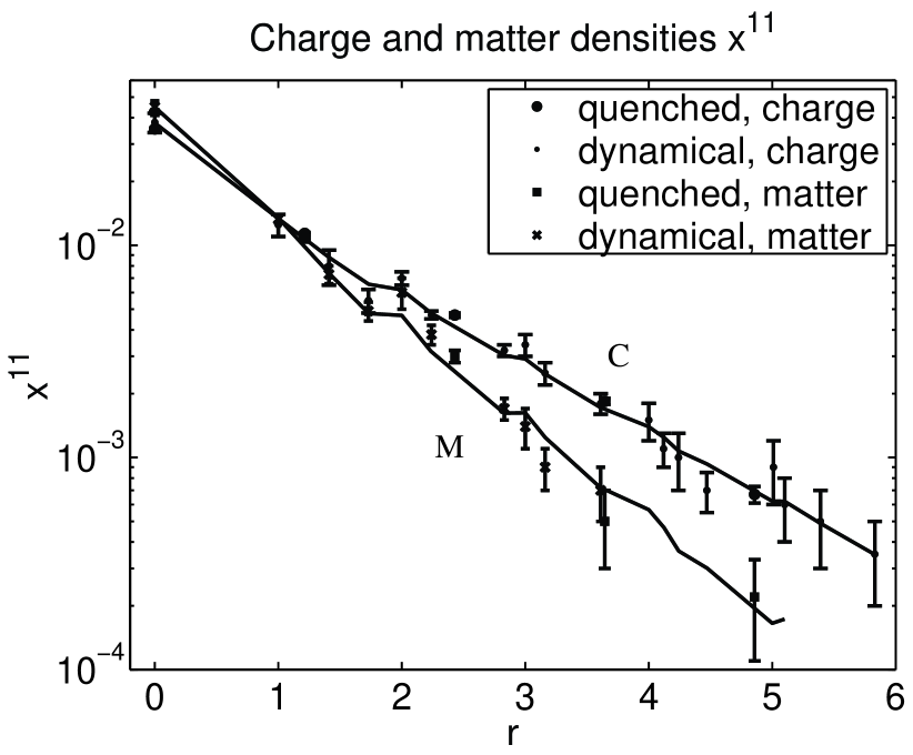
Figure 2: The radial distribution of the ground state charge (C) and matter (M) densities. The lattice exponential fits are plotted with solid lines. Here $r$ is in lattice units of $a\approx 0.14$ fm.

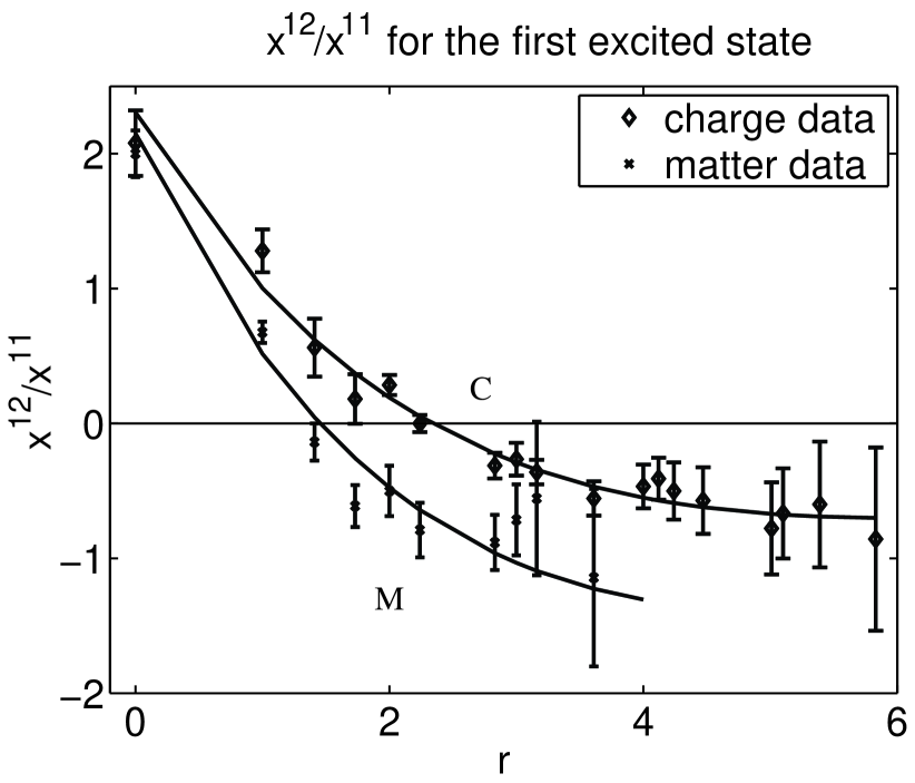
Figure 3: The ratio $x^{12}/x^{11}$ for charge (C) and matter (M) densities. The solid curves guide the eye.

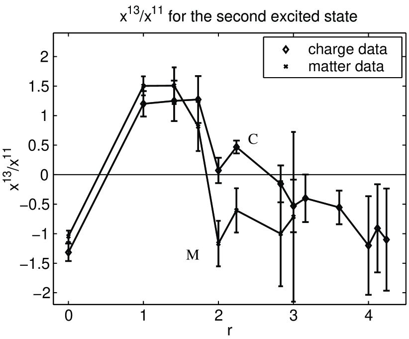
Figure 4: The ratio $x^{13}/x^{11}$ for charge (C) and matter (M) densities.

3.2 Sum rules

It is also of interest to consider the sum rules that sum over all values of $r$ i.e.

$$I_{\textrm{c(m)}}=\frac{\langle\sum_{\mathbf{r}}C_{3,c(m)}(T,\mathbf{r})\rangle}{\langle C_{2}(T)\rangle}.$$ (7)

For the charge and matter densities this yields $I_{\textrm{c}}=1.4(1)$ and $I_{\textrm{m}}=0.9(1)$ respectively. The corresponding values for the quenched approximation are $I_{\textrm{c}}=1.30(5)$ and $I_{\textrm{m}}=0.4(1)$. By charge conservation we should get $I_{\textrm{c}}=1$ in the continuum limit. Renormalisation effects of $\approx 0.7$ enter due to the finite lattice spacing.

4 CONCLUSIONS AND FUTURE

The $S$-wave charge and matter densities can be measured quite reliably out to $\approx 0.8$ fm and $\approx 0.5$ fm respectively. No difference can be seen when comparing dynamical and quenched fermions. This is probably due to the rather heavy mass of the light quarks.

This work is by no means the last word on the subject, and a lot remains to be done. The next step could be, for example, measuring the $P$-, $D$- and $F$-wave densities. The correlations in the baryonic and $(Q^{2}\bar{q}^{2})$ systems should be studied as well. We would also like to understand the densities phenomenologically using the Dirac equation. To check the continuum limit we should, of course, repeat the measurements using larger $\beta$ and bigger lattices.

The authors wish to thank the Center for Scientific Computing in Espoo, Finland for making available resources without which this project could not have been carried out. One of the authors (J.K.) wishes to thank the Magnus Ehrnrooth Foundation for financial support.

References

- [1] UKQCD Collaboration, A.M. Green, J. Koponen, P. Pennanen and C. Michael, Phys. Rev. D65 (2002), 014512 [hep-lat/0105027].
- [2] UKQCD Collaboration, A.M. Green, J. Koponen, P. Pennanen and C. Michael, ”The charge and matter radial distributions of heavy-light mesons calculated on a lattice with dynamical fermions”, [hep-lat/0206015].
- [3] C. Michael and J. Peisa, Phys. Rev. D58 (1998), 034506 [hep-lat/9802015].