ITP Budapest 586
August 2002

Lattice QCD Results at Finite Temperature and Density

Abstract

Recent lattice results on QCD at finite temperatures and densities are reviewed. Two new and independent techniques give compatible results for physical quantities. The phase line separating the hadronic and quark-gluon plasma phases, the critical endpoint and the equation of state are discussed.

1 Introduction

QCD at finite temperatures ($T$) and/or chemical potentials ($\mu$) is of fundamental importance, since it describes particle physics in the early universe, in neutron stars and in heavy ion collisions. According to the standard picture, at high $T$ and/or high density there is a transition from a state dominated by hadrons to a state dominated by partons. The expression “transition” (which occurs at the transition temperature $T_{c}$) is used for first/second order phase transitions and crossovers. (Observables change rapidly during a crossover, but no singularities appear.) Extensive experimental work has been done with heavy ion collisions at CERN and Brookhaven to explore the $\mu$-$T$ phase boundary at relatively small $\mu$ values. At large $\mu$ a rich phase structure is conjectured [1, 2, 3, 4].

There are well established nonperturbative lattice techniques to study this transition at vanishing density. At $\mu$=0 we have fairly good description of the transition (e.g. the order of the transition as a function of the quark masses or the the equation of state as a function of T). For recent reviews see the summaries of the lattice conferences [5] or the review talk on finite T lattice QCD at this conference [6].

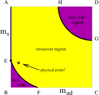
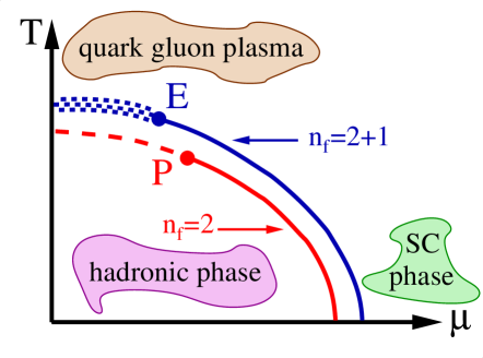
Figure 1: QCD phase diagrams. Left panel: The phase diagram on the $m_{ud}$ versus $m_{s}$ plane at $\mu$=0. The left lower and the right upper corners are first order phase transition regions. Thick solid lines (A–E,E–F and H–G) indicate second order phase transitions. The physical point is most probably in the crossover region. Right panel: The phase diagram on the T versus $\mu$ plane. For small T and $\mu$ the system is in the hadronic phase, for large T it is a quark-gluon plasma, whereas for small T and large $\mu$ colour superconductivity is conjectured. The lower curve shows the $n_{f}$=2 case. In the small $\mu$ region the dashed line indicates a second order phase transition which is connected by a tricritical point P to a first order phase transition line. The upper curve shows the $n_{f}$=2+1 case, with physical quark masses. The second order phase transition line disappears, instead of it we are faced with a crossover, illustrated by the dotted region. This region is connected to a first order phase transition line by a critical endpoint E.

Our knowledge is far more limited at nonvanishing $\mu$. Due to the sign problem (oscillating signs lead to cancellation in results, a phenomenon which appears in many fields of physics) nothing could have been said for almost 20 years about the experimentally important case at nonvanishing densities. In the last year new, and for the first time successful approaches appeared and physically relevant results were obtained [7, 8, 9, 10, 11, 12, 13].

The aim of this review is to give a self-contained picture on the lattice approach at $\mu$$\neq$0 for real QCD (QCD-like models, such as SU(2), random matrix or NJL models are not discussed). In Section 2 the qualitative features of the phase diagram are summarised both at $\mu$=0 and $\mu$$\neq$0. Section 3 briefly presents the lattice formulation and shows the associated sign problem. The main emphasis is put to the origin of the problem and technical details are not discussed. In Section 4 the two new techniques (the overlap improving multi-parameter reweighting [7] and the analytic continuation [10]) are presented. Readers who are not interested in the origin of the sign problem and in the new techniques should skip Section 3 and 4. In Section 5 results of the Budapest group [7, 8, 13] are listed (the phase line, the location of the critical endpoint and the equation of state at $\mu$$\neq$0). They are obtained by the direct application of the overlap improving multi-parameter reweighting. Section 6 gives the findings [9, 12] of the Bielefeld-Swansea group (the phase line, the equation of state at $\mu$$\approx$0 and $T$$\approx$$T_{c}$ and the response of the critical endpoint to the change of $\mu$). They also use the multi-parameter reweighting technique; however, the $\mu$-dependence of the determinant is approximated by a Taylor expansion. Section 7 discusses the phase line obtained by analytic continuation [10, 11]. Section 8 concludes.

2 Qualitative features of the phase diagram

Our knowledge on the phase diagram of QCD at $\mu$=0 and $\mu$$\neq$0 is summarized on Figure 1. Some ingredients are rigorous lattice results, others are indications from models.

What are the characteristics of the $\mu$–$T$ phase diagrams, relevant for heavy ion collisions? (See the right panel of Figure 1.) One of the most interesting features of the phase diagram is a critical endpoint E connecting the first order phase transition line with the crossover region, which separates the low T hadronic and high T quark-gluon plasma phases. It is a long-standing open question, whether such a critical point exists on the $\mu$-$T$ plane, and particularly how to predict theoretically its location [14].

Let us discuss first the $\mu$=0 case (see the left panel of Figure 1; note, that now we study only those features of the figure, which are relevant for the critical endpoint at $\mu$$\neq$0, for more details see [6] and references therein). Universal arguments [15] and lattice results [5] indicate that in a hypothetical QCD with a strange (s) quark mass ($m_{s}$) as small as the up (u) and down (d) quark masses ($m_{u,d}$) there would be a first order phase transition at finite $T$ (point in the E–B–F region). The $n_{f}$=2 case with small (but nonvanishing) u/d quark masses but with $m_{s}=\infty$ there would be no phase transition only an analytical crossover. This means that between the two extremes there is a critical strange mass ($m_{s}^{c}$) at which one has a second order finite $T$ phase transition. $n_{f}$=2+1 lattice results with two light quarks and $m_{s}$ around the $T_{c}$ indicated that $m_{s}^{c}$ is about half of the physical $m_{s}$. Thus, in the real world we probably have a crossover. (Clearly, more work is needed to approach the chiral and continuum limits [6].)

At nonvanishing $\mu$, arguments based on a variety of models predict a first order finite $T$ phase transition at large $\mu$. Combining the $\mu=0$ and large $\mu$ informations an interesting picture emerges on the $\mu$-$T$ plane. For the physical $m_{s}$ the first order phase transitions at large $\mu$ should be connected with the crossover on the $\mu=0$ axis. This suggests that the phase diagram features a critical endpoint $E$ (with chemical potential $\mu_{E}$ and temperature $T_{E}$), at which the line of first order phase transitions ($\mu>\mu_{E}$ and $T<T_{E}$) ends [14]. At this point the phase transition is of second order and long wavelength fluctuations appear, which results in characteristic experimental consequences, similar to critical opalescence. Passing close enough to ($\mu_{E}$,$T_{E}$) one expects simultaneous appearance of signatures, which exhibit nonmonotonic dependence on the control parameters [16], since one can miss the critical point on either of two sides. The location of this endpoint is an unambiguous, nonperturbative prediction of the QCD Lagrangian. Unfortunately, no ab initio, lattice work was done earlier to locate the endpoint. Only results from models [14] were available.

The goal of present $\mu$$\neq$0 lattice studies is to determine the phase diagram, to locate the endpoint and also to calculate the equation of state.

3 Lattice QCD and the sign problem at $\mu$$\neq$0

Figure 2: Illustration of Euclidean lattice QCD. Anticommuting quark fields are defined on the lattice sites. Gauge fields are SU(3) matrices and used as link variables: $U_{\nu}(n)$. The product of four links around a plaquette leads to the standard gauge action.

The continuum QCD Lagrangian in Euclidean spacetime is ${\cal L}=-{1\over 4}F_{\mu\nu}^{a}F^{a\mu\nu}+\bar{\psi}(D_{\mu}\gamma^{\mu}+m)\psi$. The first term gives the gauge, the second one the fermionic contribution. In the discretised lattice formulation the anti-commuting $\psi(n)$ quark fields live on the sites ($n$) of the lattice, whereas the $A_{\mu}^{a}$ gluon fields are used as link ($U_{\mu}(n)$) and as plaquette ($P_{\mu\nu}(n)$) variables

$$U_{\mu}(n)=\exp{(ig_{s}\int_{n}^{n+e_{\mu}}d{x^{\prime}}^{\mu}\,A_{\mu}^{a}(x^{\prime})\lambda_{a}/2)},\ \ P_{\mu\nu}(n)=U_{\mu}(n)U_{\nu}(n+e_{\mu})U^{\dagger}_{\mu}(n+e_{\nu})U^{\dagger}_{\nu}(n)$$ (1)

Here $\mu$ represents the direction and $e_{\mu}$ the corresponding unit vector. Similarly to the continuum formulation the action $S=S_{g}+S_{f}$ consists of the pure gluonic and the fermionic parts. The gluonic part is written with the help of the plaquettes: $S_{g}=6/g_{s}^{2}\cdot\sum_{n,\mu,\nu}\left[1-{\rm Re}({\rm Tr}P_{\mu\nu}(n))\right]$, where $g_{s}$ is the gauge coupling. The fermionic part on the lattice needs a differencing scheme for quarks. In the naive, noninteractive case one obtains: $\bar{\psi}(x)\gamma^{\mu}\partial_{\mu}\psi(x)\rightarrow\bar{\psi}(n)\gamma^{\mu}(\psi(n+e_{\mu})-\psi(n-e_{\mu}))$. The interacting case has $D_{\mu}$ instead of $\partial_{\mu}$, thus the gauge field is also included: $\bar{\psi}(x)\gamma^{\mu}D_{\mu}\psi(x)\rightarrow\bar{\psi}(n)\gamma^{\mu}U_{\mu}(n)\psi(n+e_{\mu})+...$ (fermion doublers do not play any role in the sign problem, therefore we do not discuss them). Fermion fields appear only in bilinear expressions, thus we can write $S_{f}=\bar{\psi}(n)M_{nm}\psi(m)$, where M is the $U$-dependent fermion matrix. Note, that the number of raws or coloumns of M is proportional to the lattice volume. In our case the matrix M is sparse, only diagonal ($\propto m$) and next-neighbour ($\propto U_{\mu}$) elements are nonvanishing.

Our system can be described by the Euclidean partition function. It is given by integrating the Boltzmann weights over the gauge and fermionic fields. The action is bilinear in the fermionic variables, thus this part of the integral can be calculated explicitely.

$${\mbox{Z}=}\int{\cal D}U{\cal D}\bar{\psi}{\cal D}\psi e^{-S_{g}-S_{f}}{\mbox{=}\int}{\cal D}Ue^{-S_{g}}\det M(U).$$ (2)

The remaining integral over the $U$ fields is calculated by stochastic methods. A canonical ensemble of field configurations is generated by Monte-Carlo algorithms. Observables are obtained as averages over the field configurations. The intrinsic feature of these techniques is importance sampling, thus we sample only the most important configurations and these individual configurations have equal weights in the averages.

We use the most straightforward technique, the Metropolis algorithm as an illustration (the Metropolis method is very CPU-intensive, thus usually faster but more complicated techniques are used). The basic step of the method is a stochastic, reversible modification of a link variable: $U_{\mu}(n)\rightarrow U^{\prime}_{\mu}(n)$. It is accepted or rejected. The Metropolis condition

$$P(U\rightarrow U^{\prime})=\min\left[1,\exp({S_{g}(U)-S_{g}(U^{\prime})})\det M(U^{\prime})/\det M(U)\right]$$ (3)

gives the probability to accept the new $U^{\prime}$ field variable. It is easy to show, that by sweeping through the whole lattice many times, we reach the canonical distribution, and physical observables can be determined. Note, that for real gauge fields $\det M(U)$ is real, thus eq. (3) really has a probability interpretation. This feature is essential not only for the Metropolis algorithm, but for any importance sampling based method.

Our primary goal is to understand QCD at finite densities. As usual, finite densities can be studied by introducing a chemical potential. One adds the following term to the continuum action: $\mu{\bar{\psi}}(x)\gamma_{4}\psi(x)$. In this formula $\mu$ acts as a fourth component of an imaginary, constant vector potential [17, 18]. As we have seen real gauge fields result in real $\det M(U)$; however, the inclusion of $\mu$ (thus a constant imaginary gauge field) gives complex $\det M(U)$. This spoils the probability interpretation of eq. (3) and any other importance sampling based method. Instead of an ensemble of equally important configurations (importance sampling) we might have configurations with complex Boltzmann weights. These complex weights with oscillating real parts largely cancel each other in observables. In the literature this phenomenon is referred to as the “sign problem”.

4 New lattice techniques at finite chemical potential

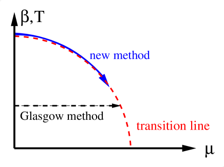
Figure 3: Illustration of the multi-parameter reweighting. The horizontal arrow shows the Glasgow, the curved one the new, multi-parameter reweighting. The dashed transition line separates the different phases. The Glasgow method starts with an ensemble in the low T, hadronic phase and uses the weighting factors of the configurations at the same T but at $\mu$$\neq$0. Clearly, the hadronic configurations do dot overlap with the transition ones. The new method starts e.g. at the transition point at $\mu$=0 and changes T and $\mu$ simultaneously, keeping the system on the transition line. The overlap is much better.

The overlap improving multi-parameter reweighting [7] opened the possibility to study lattice QCD at nonzero $T$ and $\mu$. First one produces an ensemble of QCD configurations at $\mu$=0 and at T$\neq$0. Then the Ferrenberg-Swendsen type reweighting factors [19] of these configurations are determined at $\mu$$\neq 0$ and at a lowered T. The idea can be easily expressed in terms of the partition function

$$Z(\mu,\beta)=\int{\cal D}U{\rm e}^{-S_{g}(\beta,U)}\det M(\mu,m,U)=$$ (4)

$$\int{{\cal D}U{\rm e}^{-S_{g}(\beta_{0},U)}\det M(\mu=0,m,U)}{\left\{{\rm e}^{-S_{g}(\beta,U)+S_{g}(\beta_{0},U)}\frac{\det M(\mu,m,U)}{\det M(\mu=0,m,U)}\right\}},$$

where $S_{g}(U)$ is the action of the gluonic field, $\beta=6/g^{2}$ fixes the coupling of the strong interactions ($g$). Note that for a given lattice $T$ is an increasing function of $\beta$. The quark mass parameter is $m$ and $\det M$ comes from the integration over the quark fields (see eq.(2)). At nonzero $\mu$ one gets a complex $\det M$ which has no probability interpretation, thus it spoils any importance sampling. Thus, the first line of eq. (4) at $\mu$$\neq$0, is rewritten in a way that the first part of the second line is used as an integration measure (at $\mu$=0, for which importance sampling works) and the remaining part in the curly bracket is measured on each configuration and interpreted as a weight factor $\{w(\beta,\mu,m,U)\}$. (For $n_{f}$$\neq$4 fractional powers of $\det M$ is needed. This complication can be solved [8].)

The reweighting is performed along the best weight lines on the $\mu$–$\beta$ plane (or equivalently on the $\mu$–$T$ plane). One such line is the transition line. The best weight lines are determined by minimising the spread of $\log w$. The technique works for $T$ at, below and above $T_{c}$. Using the above weights any observable ${\cal O}$ can be determined at $\mu$$\neq$0

$${\overline{\cal O}}(\beta,\mu,m)=\frac{\sum\{w(\beta,\mu,m,U)\}{\cal O}(\beta,\mu,m,U)}{\sum\{w(\beta,\mu,m,U)\}}.$$ (5)

The method is illustrated on Fig. 3. Using multi-parameter reweighting one simultaneously changes T and $\mu$. A much better overlap can be obtained by the multi-parameter reweighting than by the single $\mu$-reweighting Glasgow-method [20]. The Glasgow-method reweights pure hadronic configurations to transition ones. By the new technique transition (or hadronic/QGP) configurations are reweighted to transition (or hadronic/QGP) ones. Since the original ensemble is collected at $\mu$=0 one does not expect that even the new technique is able to describe the physics of the large $\mu$ region with e.g. colour superconductivity. Fortunately, the typical $\mu$ values at present heavy ion accelerators are smaller than the covered region.

An alternative approach [9] uses Taylor expansion of eqs. (4,5) as a function of $\mu$ (or $m$) and hence estimates the derivatives of various quantities with respect to $\mu$ (or $m$). Thus, for the case of a Taylor expansion in $\mu$ one has

$$\ln\left({{\det M(\mu)}\over{\det M(0)}}\right)=\sum_{n=1}^{\infty}\frac{\mu^{n}}{n!}\frac{\partial^{n}\ln\det M(0)}{\partial\mu^{n}}\equiv\sum_{n=1}^{\infty}{R}_{n}\mu^{n}.$$ (6)

Instead of using the explicit form of the determinants in eq. (4) the Bielefeld-Swansea group used the derivatives in $\mu$. Compared to the explicit calculation of the determinants, the Taylor technique needs less CPU-time (derivatives can be estimated stochastically); however, only valid for somewhat smaller $\mu$ values than the full technique.

The other promising and absolutely independent approach is the analytic continuation from imaginary to real chemical potentials [10]. One computes first the critical line for imaginary chemical potential. For these $\mu$ values there is no sign problem, therefore Monte-Carlo simulations based on importance sampling can be carried out. One can check the convergence of the Taylor expansion of the critical line, thus $\beta_{c}$ as a function of Im($\mu$). The convergence seems to be surprisingly fast for the whole range of chemical potentials accessible to this method. Analytic continuation of the Taylor series then reduces to simply flipping the sign of the appropriate terms. Finally, the infinite volume limit has to be taken from the continued results at real $\mu$. Using this technique the phase line separating the hadronic and quark-gluon plasma phases were determined [10, 11]. The order of the transition can then be determined in a $(V,\mu)$-range where the truncation error of the series is smaller than finite size scaling effects.

5 Overlap improving multi-parameter reweighting: direct approach

This section summarizes some results of the Budapest group [7, 8, 13] obtained in 2+1 flavour dynamical staggered QCD on $N_{t}$=4 lattices.

Figure 4: The T-$\mu$ diagram. Direct results are given with errorbars. Dotted line at small $\mu$ shows the crossover, solid line at larger $\mu$ the first order transition. The box gives the uncertainties of the endpoint.

Figure 4 shows the phase diagram on the $\mu$–T plane in physical units, thus $T_{c}$ as a function of $\mu_{B}$, the baryonic chemical potential (which is three times larger then the quark chemical potential). The analysis is consisted of three steps. First one determines the transition points as a function of $\mu$. Then the $V\rightarrow\infty$ behaviour is inspected to separate the crossover and the first order phase transition region. Finally one transforms lattice units into physical ones. In physical units the endpoint [8] is at $T_{E}=160\pm 3.5$ MeV, $\mu_{E}=725\pm 35$ MeV. At $\mu_{B}$=0 we obtained $T_{c}=172\pm 3$ MeV. Note, that due to CPU-limitations in this analysis the light quark masses are approximately three times larger than their physical value and the lattice spacing is $\approx$0.28 fm. Clearly more work is needed to extrapolate to the thermodynamic, chiral and continuum limits.

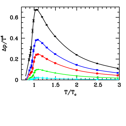
\begin{picture}(17.0,0.1)\end{picture}

Figure 5: Left panel: $p/T^{4}$ as a function of $T/T_{c}$ at $\mu=0$ The continuum SB limit is also shown. Right panel: $\Delta p=p(\mu\neq 0,T)-p(\mu=0,T)$ normalized by $T^{4}$ as a function of $T/T_{c}$ for $\mu_{B}$=100,210,330,410 MeV and $\mu_{B}$=530 MeV (from bottom to top).

The equation of state at $T\neq 0$ and $\mu\neq 0$ is also determined [13]. In order to help the continuum interpretation of the figures we normalize the raw lattice results with the dominant correction factors between $N_{t}$=4 and the continuum in the $T\rightarrow\infty$ (Stefan-Boltzmann; SB) case (see Ref. [13]). Therefore, the results presented on the figures might be interpreted as continuum estimates and could be directly used in phenomenological applications.

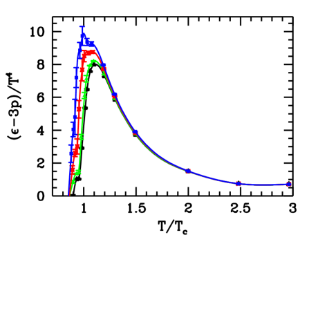
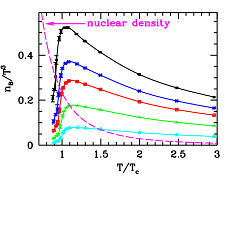
Figure 6: Left panel: $(\epsilon-3p)/T^{4}$ at $\mu_{B}$=0,210,410 MeV and $\mu_{B}$=530 MeV as a function of $T/T_{c}$ (from bottom to top). Right panel: The baryon number density normalized by $T^{3}$ as a function of $T/T_{c}$ for $\mu_{B}=$100,210,330,410 MeV and $\mu_{B}$=530 MeV. As a reference value the line starting in the left upper corner indicates the nuclear density.

Figure 5 shows the pressure ($p$) at $\mu$=0 and $\Delta p$($T$,$\mu$)=$p$($T$,$\mu$)-$p$($T$,$\mu$=0) normalized by $T^{4}$. Note, that normalizing $\Delta p$($T$,$\mu$) by $\Delta p$($T\rightarrow\infty$,$\mu$) leads to an almost universal $\mu$-independent function [13]. The left panel of Figure 6 shows $\epsilon$-3$p$ normalized by $T^{4}$, which tends to zero for large $T$ ($\epsilon$ is the energy density). The right panel gives the baryon number density as a function of $T/T_{c}$ for different $\mu$-s. As it can be seen the densities exceed the nuclear density by up to an order of magnitude.

6 Overlap improving multi-parameter reweighting: Taylor expansion

Figure 7: Left panel: The $\mu$ dependence of the chiral susceptibility. Right panel: Transition temperature as a function of $\mu$. The $\mu$ value of RHIC is indicated by an arrow.

This section summarizes some results of the Bielefeld-Swansea group [9, 12] obtained in dynamical staggered QCD with p4 action on $N_{t}$=4 lattices.

Instead of evaluating the determinants in eq. (4) explicitely one can approximate them by using a Taylor expansion as given by eq. (6). One calculates observables as a function of $\mu$ using eq. (5). The left panel of Figure 7 shows the chiral susceptibility as a function of the gauge coupling for three different $\mu$ values. Note, that the peak indicates the transition and that its position moves as $\mu$ changes. Since the gauge coupling is directly connected to T one can convert the position of the peaks into physical units and obtain the $T_{c}$ as a function of $\mu$ (right panel of Figure 7). The authors of Ref. [9] concludes that the curvature of the phase diagram at $\mu$=0 is in good agreement with that of Ref. [8] (they show the endpoint of Ref. [8] by a diamond signaled as Fodor & Katz).

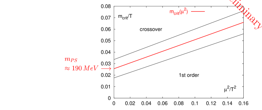
Figure 8: $m_{crit}/T$ as a function of $\mu^{2}/T^{2}$. The band indicates the uncertainties.

The equation of state was also studied at small $\mu$ values. At the RHIC point both $\epsilon$ and $p$ increase by around 1% from its $\mu$=0 value. Along the transition line their change is consistent with zero within the current precision [9].

In a hypothetical QCD with degenerate quark masses and $m_{\pi}$$\approx$$m_{K}$$\approx$190 MeV the critical endpoint is at $\mu$=0. Note, that $\mu$$\neq$0 values correspond to larger critical masses ($m_{crit}$). A preliminary result is shown in Figure 8. Using the $\mu$ dependence of $m_{crit}$ one could, in principle, estimate the location of the endpoint for physical quark masses.

7 Analytic continuation from imaginary $\mu$

This section summarizes the results obtained by the analytic continuation technique. $N_{t}$=4 lattices are used with 2 flavour [10] and 4 flavour [11] dynamical staggered QCD.

In Ref. [10] an alternative approach was developed, avoiding reweighting in $\mu$ altogether. This is achieved by simulating with imaginary $\mu$, where there is no sign problem and hence no need for reweighting. In this case one may fit the nonperturbative data of an observable (even of the critical line) by truncated Taylor series in $\mu/T$ (see left panel of Figure 9). In the absence of nonanalyticities, the series may be analytically continued to real values of $\mu$ (right panel of Figure 9). For the transition temperature [10] one gets $T_{c}(\mu)=T_{c}(0)-0.0056\mu^{2}/T$ (note, that similar value was obtained in four flavour QCD by Ref. [11]). These results are in complete agreement with those of the previous two sections.

Performing the analytic continuation for different volumes, a finite volume scaling analysis should reveal the nature of the transition. In particular, it might then be possible to locate the critical endpoint by this technique, too.

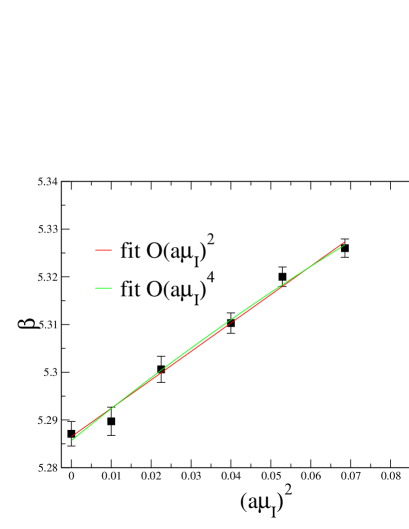
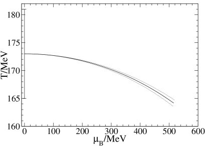
Figure 9: Left panel: Transition coupling for imaginary $\mu$ with different fits. Right panel: Transition temperature in physical units for $\mu$$\neq$0.

8 Conclusions

Due to the notorious sign problem this is the first time that basic thermodynamic quantities could be obtained on the lattice at finite chemical potentials. Completely different new techniques lead to very similar result, which indicates that in the near future lattice QCD could be a major contributor to the field. Clearly, more work has to be done in order to reach the thermodynamic, chiral and continuum limits.

Acknowledgements: The work has been partially supported by Hungarian Scientific grants, OTKA-T34980/T29803/M37071/OMFB1548/OMMU-708. Preliminary results from the Bielefeld-Swansea group are also acknowledged [12].

References

- [1] M. G. Alford, K. Rajagopal and F. Wilczek, Phys. Lett. B 422 (1998) 247.
- [2] M. G. Alford, K. Rajagopal and F. Wilczek, Nucl. Phys. B 537 (1999) 443.
- [3] R. Rapp, T. Schafer, E. V. Shuryak and M. Velkovsky, Phys. Rev. Lett. 81 (1998) 53.
- [4] K. Rajagopal and F. Wilczek, arXiv:hep-ph/0011333.
- [5] For recent reviews see: A. Ukawa, Nucl. Phys. Proc. Suppl. 53, 106 (1997); E. Laerman, ibid. 63, 114 (1998); F. Karsch, ibid. 83, 14 (2000); S. Ejiri, ibid. 94, 19 (2001).
- [6] K. Kanaya, these proceedings.
- [7] Z. Fodor and S. D. Katz, Phys. Lett. B 534 (2002) 87 [arXiv:hep-lat/0104001].
- [8] Z. Fodor and S. D. Katz, JHEP 0203 (2002) 014 [arXiv:hep-lat/0106002].
- [9] C. R. Allton et al., arXiv:hep-lat/0204010.
- [10] P. de Forcrand and O. Philipsen, arXiv:hep-lat/0205016.
- [11] M. D’Elia and M.P. Lombardo, hep-lat/0205022; for the phase diagram continued to real see their poster at this conference.
- [12] C. Schmidt, talk presented at the Lattice’02 conference (Boston, July 2002).
- [13] Z. Fodor, S.D. Katz and K.K. Szabó, arXiv:hep-lat/0208078.
- [14] M. Halasz et al. Phys. Rev. D58 (1998) 096007; J. Berges and K. Rajagopal, Nucl. Phys. B538 (1999) 215; M. Stephanov, K. Rajagopal and E. Shuryak, Phys. Rev. Lett. 81 (1998) 4816.
- [15] R. Pisarski and F. Wilczek, Phys. Rev. D29 (1984) 338; F. Wilczek, Int. J. Mod. Phys. A7 (1992) 3911; K. Rajagopal and F. Wilczek, Nucl. Phys. B399 (1993) 395.
- [16] M. Stephanov, K. Rajagopal and E. Shuryak, Phys. Rev. D60 (1999) 114028.
- [17] P. Hasenfratz and F. Karsch, Phys. Lett. B 125 (1983) 308.
- [18] J. B. Kogut et al., Nucl. Phys. B 225 (1983) 93.
- [19] A. M. Ferrenberg and R. H. Swendsen, Phys. Rev. Lett. 61 (1988) 2635.
- [20] I. M. Barbour et al., Nucl. Phys. Proc. Suppl. 60A (1998) 220 [arXiv:hep-lat/9705042].