Quenched QCD with fixed-point and chirally improved fermions

Abstract

In this contribution we present results from quenched QCD simulations with the parameterized fixed-point (FP) and the chirally improved (CI) Dirac operator. Both these operators are approximate solutions of the Ginsparg-Wilson equation and have good chiral properties. We focus our discussion on observables sensitive to chirality. In particular we explore pion masses down to 210 MeV in light hadron spectroscopy, quenched chiral logs, the pion decay constant and the pion scattering length. We discuss finite volume effects, scaling properties of the FP and CI operators and performance issues in their numerical implementation.

1 Introductory remarks

Fixed point [1, 2, 3, 4] and chirally improved fermions [5, 6] provide an approach to chiral symmetry on the lattice based on the Ginsparg-Wilson equation [7]. In an actual implementation both the FP and CI fermions give rise to an approximate solution of this equation and it has to be tested how well a chiral fermion is described by such an approximation. Here we report on our results from quenched QCD calculations focussing in particular on observables sensitive to chiral symmetry (for a recent general review of results with chiral actions see [8]).

In another contribution to these proceedings [9] we gave a more general overview of our calculations and also a brief introduction to the construction of the FP and CI operators ($D_{FP}$, $D_{CI}$). Here we would like to deepen the discussion and present selected topics in more detail. These topics include light hadron spectroscopy, the quenched chiral logarithm, the pion decay constant and a preliminary study of the $I=2$ pion scattering length.

Both the FP and the CI operators make use of the full Clifford algebra and a large number of gauge paths to approximate a solution of the Ginsparg-Wilson equation. They differ in the method for determining the coefficients in front of the individual terms of the Dirac operator. The FP operator is constructed from classical equations which determine the fixed point of a renormalization group transformation in QCD. For the CI operator the Ginsparg-Wilson equation is mapped onto a system of coupled equations for the coefficients of the individual terms of the Dirac operator and this system is then solved numerically. In our implementation of the two operators we restrict ourselves to terms essentially on the hypercube only. For a more detailed discussion of the operators see [1, 2, 3, 4, 5, 6, 9].

$D$	$N_{s}^{3}\times N_{t}$	$a(r_{0})$	#conf	$m_{\rm PS}/m_{\rm V}$
FP	$16^{3}\times 32$	0.16 fm	200	0.28–0.88
FP	$12^{3}\times 24$	0.16 fm	200	0.3–0.88
ov3	$12^{3}\times 24$	0.16 fm	100	0.21–0.88
FP	$8^{3}\times 24$	0.16 fm	200	0.3–0.88
FP	$12^{3}\times 24$	0.10 fm	200	0.34–0.89
FP	$16^{3}\times 32$	0.08 fm	100	0.36–0.89
CI	$16^{3}\times 32$	0.15 fm	100	0.38–0.85
CI	$12^{3}\times 24$	0.15 fm	100	0.36–0.85
CI	$8^{3}\times 24$	0.15 fm	200	0.33–0.85
CI	$16^{3}\times 32$	0.10 fm	100	0.33–0.92
CI	$12^{3}\times 24$	0.10 fm	100	0.32–0.92
CI	$16^{3}\times 32$	0.08 fm	100	0.40–0.95

Table 1: Statistics for the FP and CI Dirac operator together with the lattice spacing measured with the Sommer parameter and the range of pseudoscalar to vector mass ratios we worked at.

The parameters of our quenched QCD calculations were chosen similar for the two operators such that a direct comparison of the results is possible. For both operators we used lattices of size $8^{3}\times 24$, $12^{3}\times 24$, $16^{3}\times 32$ with lattice spacings of approximately $a=0.08$ fm, $0.10$ fm and $0.15$ fm. Thus, we were able to study finite volume effects (constant $a$) as well as discretization effects (constant physical volume). The FP operator was used together with quenched configurations from a parameterized perfect gauge action [10] subsequently smoothened with renormalization group inspired smearing [3]. The latter can be viewed as part of the parameterization of the FP operator. We also employed a version of the FP operator (ov3) augmented with overlap steps [11]. It is constructed from the parameterized FP operator with three terms of the Legendre expansion of the overlap. For the chirally improved operator we generated the quenched gauge configurations with the Lüscher-Weisz gauge action [12] and applied one step of HYP blocking [13] to improve the properties of the Dirac operator. An overview of the statistics is given in Table 1. There we also give the results for the lattice spacing as determined from the Sommer parameter [10, 14] and the range of pseudoscalar to vector meson mass ratios we have worked at. The smallest pion mass we have worked at is 210 MeV for the FP operator (160 MeV with ov3) and 240 MeV for the CI operator. We did not encounter problems with exceptional configurations for the listed range of pion masses and we expect that we can reach pion masses of 200 MeV for both operators without having to go to exceedingly small lattice spacings.

Our hadron propagators were created by smeared sources. For the FP operator we fixed the gauge configurations to Coulomb gauge and used Gaussian sources. For the CI operator we employed Jacobi smearing [15] and no gauge fixing was necessary.

At every fermion offset of the hypercube a large number of gauge paths contribute in our Dirac operators. By precalculating and storing some basic gauge link products the construction of the corresponding sparse matrix could be speeded up significantly. Every offset on the hypercube is represented by a color-Dirac matrix whose size is $12\times 12$ independently of the number of gauge paths to this offset. When comparing the cost to e.g. the Wilson operator (without clover term) the number of floating point operations in the basic matrix-vector multiplication is increased by a factor of $\approx 36$. However, since the bottleneck is the access to memory and we do more operations with each SU(3) matrix we fetch from memory (all 16 entries in the Dirac space are used, Wilson uses only 4) the actual number might be quite different. Furthermore we observed [3] that some numerical operations such as the computation of low lying eigenvalues converge considerably faster for our Dirac operators than for Wilson’s operator.

Our calculations were done on the Hitachi SR8000 at the Leibniz Rechenzentrum in Munich and the production runs were typically performed on 8 to 16 nodes each consisting of 8 CPUs with shared memory. The Dirac operator was distributed among the nodes and the parallelization was done using MPI.

2 Pion masses

2.1 Different correlators for the pion

In order to extract the pion we experimented with different operators which have overlap with this channel. In Fig. 1 we compare the effective mass plots at different bare quark masses obtained for three combinations of sources and sinks constructed from the point-like pseudoscalar and axial-vector densities. The mass plateaus are quite well pronounced although for the third correlator the signal is noisier as it is expected for a correlator with additional derivatives.

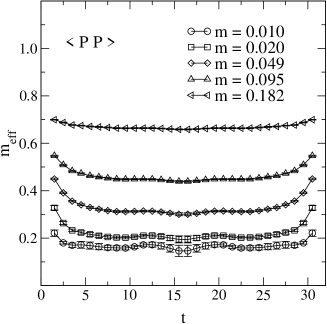
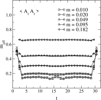
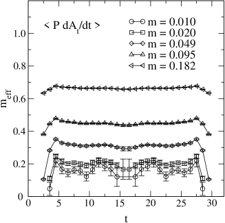
Figure 1: Effective mass plots for three different correlation functions (top to bottom: $\langle\,P\,P\,\rangle$, $\langle\,A_{t}\,A_{t}\,\rangle$, $\langle\,P\,\partial_{t}A_{t}\,\rangle$) for $D_{CI}$, $16^{3}\times 32$, $\beta_{LW}=8.7$, $a=0.08~{}\textrm{fm}$; they demonstrate the pion content of the involved operators. As expected the signal becomes noisier from top to bottom.

The masses corresponding to the 2-point functions were extracted from overall fits to cosh-behaviour covering lattice distances between $(t_{\rm min},t_{\rm max})$. These parameters were fixed by inspecting the effective mass plots and checking the $\chi^{2}$ of the fit. In Fig. 2 we compare the masses from the three correlators and find that they agree within errors.

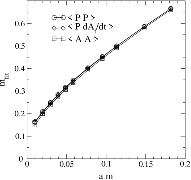
Figure 2: Pion masses obtained from different correlators ($D_{CI}$, $16^{3}\times 32$, $\beta_{LW}=8.7$, $a=0.08~{}\textrm{fm}$).

2.2 Zero mode effects in pion correlators

In the chiral region the pion correlators suffer from a topological finite size effect specific to the quenched approximation [16, 17]. Zero modes of the Dirac operator (suppressed by the fermion determinant in a dynamical calculation) lead to an unphysical increase in the pion mass at small quark masses. Since the abundance of zero modes scales only as $\sqrt{V}$ with the volume, the net effect goes as $1/\sqrt{V}$. For small volumes, however, this effect is quite important.

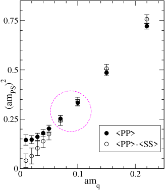
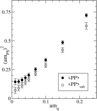
Figure 3: Effect of the subtraction of the zero modes on the pion mass (FP-ov3 operator $6^{3}\times 16$, $a=0.16~{}\mathrm{fm}$). The mass from $G_{PP}$ is represented by filled circles, while we use open circles to represent the results from the subtracted correlator of Eq. (1) (top plot), and from the explicit removal of the zero modes from the quark propagators (bottom plot).

Removing simply the contribution of the zero modes from the quark propagator is a dangerous procedure since it might change the pion propagator in a non-local manner. Another possibility is [16, 17] to consider the difference of the pseudoscalar and scalar 2-point functions

$$G_{PP-SS}=G_{PP}-G_{SS}\ .$$ (1)

This method is based on the fact that for exactly chirally symmetric actions the scalar propagator has the same topological finite size effect as the pseudoscalar propagator, while for small quark masses the lightest particle in this channel is much heavier than the pion. This observation suggests the following strategy. At small quark masses, where $G_{PP}$ is strongly distorted, we determine the pion mass from $G_{PP-SS}$. Going towards heavier quark masses the significance of the zero modes is suppressed and we expect a window where $G_{PP}$ and $G_{PP-SS}$ lead to consistent mass fits. In this window and beyond it we use the $G_{PP}$ correlator. At heavy quark masses the mass difference between the pseudoscalar and scalar masses is too small to be resolved and the fitted mass from $G_{PP-SS}$ would be larger than the true pseudoscalar mass. Fig. 3 illustrates these expectations on a small lattice for the FP-ov3 operator. In the top plot the circle indicates the window where the zero mode effects are already negligible, but the scalaris much heavier than the pion and so the correct pion mass is easily seen in the $G_{PP-SS}$ correlator. The bottom figure illustrates the danger of separating modes from the quark propagator itself: although at small quark masses one obtains the same pion mass as from $G_{PP-SS}$, at intermediate and large quark masses the pion mass obtained is incorrect. No window exists in this case.

Once the lattice volume is sufficiently large the topological finite size effect is no longer visible. In Fig. 4 we show the pion mass for a box with spatial extent of $L=2.6$ fm ($16^{3}\times 32$ lattice, $a=0.16$ fm, FP operator). The data is fitted with a quadratic polynomial (full curve) and also a curve including the quenched chiral log [18] (dashed curve). Although the difference between these fits is not seen on the scale of the figure, the quality of the $Q\chi PT$ fit is significantly better. Both curves extrapolate reasonably well to zero with the quark mass indicating that the topological finite size effect is negligible in this large box. In principle one can determine the quenched chiral log parameter directly from the pion with degenerate quark masses (see e.g. [19] for recent such determinations with the overlap operator) but in the next section we study the quenched chiral logs using a more effective method. Fig. 4 also includes data for the axial Ward identity (AWI) mass (crosses) which we will discuss later.

Figure 4: Pion mass (circles) and AWI mass (crosses) as a function of the bare quark mass. $16^{3}\times 32$ lattice, $a=0.16$ fm, FP operator.

2.3 Quenched chiral logs

Figure 5: $x-y$ plot for the FP operator ($16^{3}\times 32$ lattice, $a=0.16$ fm).

Let us now discuss the determination of the quenched chiral log parameter $\delta$ with a different method [21]. The idea is to use not only data for the pion with degenerate quark masses but to also take into account data computed with non-degenerate quark masses. The prediction from quenched chiral perturbation theory for the dependence of the pseudoscalar meson mass $m_{\mathrm{PS},12}$ on the quark masses $m_{1}$ and $m_{2}$ reads [18]

$$\begin{split}&m_{\mathrm{PS},12}^{2}=\\ &A(m_{1}+m_{2})\Big{\{}1-\delta\big{[}\ln{\frac{2m_{1}A}{\Lambda_{\chi}^{2}}}+\frac{m_{2}}{m_{2}-m_{1}}\ln{\frac{m_{2}}{m_{1}}}\big{]}\\ &+\frac{1}{A}\alpha_{X}\big{[}m_{1}\ln{\frac{2m_{1}A}{\Lambda_{\chi}^{2}}}+m_{2}\ln{\frac{2m_{2}A}{\Lambda_{\chi}^{2}}}\\ &+\frac{m_{1}m_{2}}{m_{2}\!-\!m_{1}}\ln\frac{m_{2}}{m_{1}}\big{]}\Big{\}}+B(m_{1}\!+\!m_{2})^{2}+{\cal O}(m^{3},\delta^{2}),\end{split}$$ (2)

with $A$, $B$, $\delta$ and $\alpha_{X}$ a priori unknown constants. The arbitrary scale $\Lambda_{\chi}$ is of the order $1~{}\mathrm{GeV}$. The dependence on the constants $A$, $B$ and $\Lambda_{\chi}$ can be removed by forming the following cross ratio $y$ [21]:

$$y=\frac{2m_{1}}{m_{1}+m_{2}}\frac{m_{\mathrm{PS},12}^{2}}{m_{\mathrm{PS},11}^{2}}\frac{2m_{2}}{m_{1}+m_{2}}\frac{m_{\mathrm{PS},12}^{2}}{m_{\mathrm{PS},22}^{2}}\;.$$ (3)

For small $\delta$, $\alpha_{X}$ and small quark masses $y$ is expected to behave like

$$y=1+\delta x+\alpha_{X}z+{\cal O}(m^{2},\delta^{2})$$ (4)

with

$$\!\!x \!=\! 2+\frac{m_{1}+m_{2}}{m_{1}-m_{2}}\ln\left(\frac{m_{2}}{m_{1}}\right)\;,$$ (5)

$$\!\!z \!=\! \frac{1}{A}\left(\frac{2m_{1}m_{2}}{m_{2}-m_{1}}\ln\frac{m_{2}}{m_{1}}\!-\!m_{1}-m_{2}\right),$$ (6)

which means that $\delta$ can be extracted for small quark masses from the slope of $y$ as a function of $x$. Since in this analysis the quark mass enters only in ratios, for $m_{1}$ and $m_{2}$ any definition can be used where the quark mass has no additive renormalization. (The multiplicative quark mass renormalization cancels.) The mass $m_{AWI}$ defined by the axial Ward identity has this property and was used when comparing Eq. (4) with the data. The plots are shown in Fig. 5 for the FP operator ($16^{3}\times 32$ lattice, $a=0.16$ fm) and in Fig. 6 for the CI operator ($16^{3}\times 32$ lattice, $a=0.15$ fm). Suppressing $\alpha_{X}z$ and other higher order terms in Eq. (4) we find $\delta=0.17(2)$ for the FP operator and $\delta=0.18(3)$ for the CI operator.

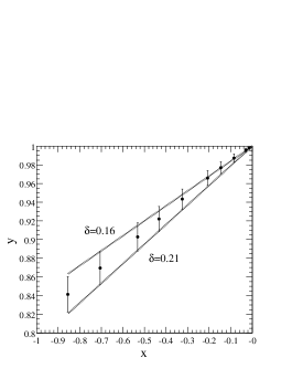
Figure 6: $x-y$ plot for the CI operator ($16^{3}\times 32$ lattice, $a=0.15$ fm).

We have not yet studied the systematical errors of these predictions due to cut-off or chiral symmetry breaking effects (our Dirac operators satisfy the Ginsparg-Wilson relation approximately only). Further, the data with large negative $x$ come from large ratios of the two quark masses which implies in our case that one of the quark masses is large, stretching the validity of Eq. (2).

3 Pion decay constant

3.1 The residual quark mass

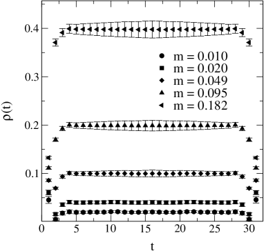
Figure 7: Results for the ratio $\rho(t)$ for $D_{CI}$, $16^{3}\times 32$, $\beta_{LW}=8.7$, $a=0.08~{}\textrm{fm}$.

For a chirally symmetric theory one may define conserved, covariant currents which do not require renormalization and covariant scalar and pseudoscalar densities whose renormalization factors satisfy $Z_{S}=Z_{P}=1/Z_{m}$ [24, 4]. Here $Z_{m}$ is the renormalization factor of the quark mass which is the coefficient of the covariant scalar density in the Dirac operator. Although the overhead using such currents and densities is expected to be relatively small [4] we used point-like, non-conserved and non-covariant operators in this work. (The mass operator in the action is, however, covariant.)

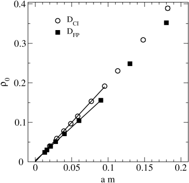
Figure 8: The plateau values for the ratio $\rho_{0}(m)\equiv 2\,m_{AWI}(m)$ vs. the bare quark masses for both Dirac operators $D_{CI}$ ($\beta_{LW}=7.9$, $a=0.15~{}\textrm{fm}$) and $D_{FP}$ ($\beta_{FP}=3.0$ , $a=0.16~{}\textrm{fm}$) for lattice size $16^{3}\times 32$. The linear fit indicates a very small residual quark mass.

In Fig. 7 we show the ratio

$$\rho(t)=\frac{\langle P^{-}(0)\,\partial_{t}A^{+}_{t}(\vec{p}=0,t)\rangle}{\langle P^{-}(0)\,P^{+}(\vec{p}=0,t)\rangle}$$ (7)

where $P$ and $A_{t}$ are the pseudoscalar density and the time component of the axial-vector current, respectively and $P^{\pm}=P^{1}\pm iP^{2}$, where 1,2 are flavor indices. This quantity exhibits excellent plateaus for separations above 3 lattice spacings. We denote the plateau values by $\rho_{0}$. The sources $P(0)$ are smeared, the sink operators unsmeared.

For renormalized fields the ratio is just twice the renormalized quark mass (see also the discussion in the next section); in fact, $\rho_{0}/2$ may be employed to define a bare mass parameter. This mass has no additive renormalization: $\rho_{0}/2=0$ if $m_{\pi}=0$. We have referred to this mass before as the Ward identity mass $m_{AWI}$. We identify the residual quark mass for our Dirac operators by the value of the bare quark mass in the action for which $\rho_{0}/2=0$. Fig. 8 gives an example of our results, both for $D_{CI}$ and $D_{FP}$ (at slightly different lattice spacings) and we find linear behaviour for small bare quark masses. A linear fit to these data and data for other parameters demonstrates a very small residual quark mass shift ranging for $D_{CI}$ from 0.002(1) at $a=0.15~{}\textrm{fm}$ to 0.000(1) at $a=0.08~{}\textrm{fm}$, and for $D_{FP}$ from -0.0006(4) at $a=0.16~{}\textrm{fm}$ to -0.0194(2) at $a=0.08~{}\textrm{fm}$. The largest value for $D_{FP}$ is likely related to the fact that $D_{FP}$ was optimized at $a=0.16~{}\textrm{fm}$ and then also used at the smaller lattice spacing without readjustment.

3.2 $Z_{A}$ and $f_{\pi}$

Exact chiral symmetry on the lattice implies that the covariant conserved axial current and the covariant pseudoscalar density satisfy the equation

$$\partial_{\mu}\,\tilde{A}^{\pm}_{\mu}(x)=2\,m\,\tilde{P}^{\pm}(x)\;,$$ (8)

which can be used in on-mass-shell Green’s functions, or put differently, Eq. (8) is valid in general bare Green’s functions up to contact terms. In this equation $m$ is the bare quark mass multiplying the covariant scalar density in the Dirac operator, $\tilde{A}_{\mu}$ is the covariant conserved current and $\tilde{P}$ is the covariant density. Eq. (8) is a consequence of bare Ward identities which follow directly from the path integral formulation of lattice QCD with Ginsparg-Wilson fermions.

Considering Eq. (7) with such covariant and conserved operators we get $2m$ on the left hand side. Replacing the conserved covariant current on the r.h.s. by $Z_{A}A_{t}$, where $A_{t}$ is the naive point-like current, we can calculate $Z_{A}$ in terms of the correlators and $m$. It can be shown [4] that, for $2R=1$ in the Ginsparg-Wilson relation as it is the case for $D_{CI}$, in these correlators the covariant pseudoscalar density can be replaced by the naive point-like density divided by $(1-m/2)(1-m^{2}/4)$. This factor goes to 1 in the chiral or in the continuum limit. At the end the renormalization factor $Z_{A}$ of the point-like current can be obtained by measuring correlators of the point-like operators. Up to factors ($\approx 1$) mentioned above $Z_{A}=2m/\rho_{0}$, where $\rho_{0}$ is the plateau of the ratio in Eq. (7) discussed in the previous section. We collected the corresponding numbers in Table 2. These numbers might be distorted by the small chiral symmetry breaking effects in $D_{CI}$. The trick of replacing the covariant densities by their naive point-like versions is modified for the case when $2R$ is a non-trivial local operator [4] as it is the case for $D_{FP}$. For the FP action the corresponding correlators are not yet measured.

$D_{CI}$
$N_{s}^{3}\times N_{t}$	$a=$	$0.15~{}\textrm{fm}$	$0.10~{}\textrm{fm}$	$0.08~{}\textrm{fm}$
$8^{3}\times 24$		0.94(2)
$12^{3}\times 24$		1.00(2)	0.96(1)
$16^{3}\times 32$		1.00(2)	0.97(1)	0.96(1)

Table 2: Values for the renormalization factor $Z_{A}$ of the point-like axial current for $D_{CI}$.

Similar considerations can be used to connect $f_{\pi}$ with the correlator of point-like, naive pseudoscalar densities. Start with the correlator $\sum_{\vec{x}}\langle\tilde{P}(\vec{x},t)\tilde{P}(0)\rangle$ where $\tilde{P}$ is the covariant density entering the AWI. Saturating this correlator by the pion intermediate state for large time separation, using Eq. (8) and the definition of the pion decay constant one obtains

$$\begin{array}[]{l}\sum_{\vec{x}}\langle\tilde{P}^{-}(\vec{x},t)\tilde{P}^{+}(0)\rangle\cr\displaystyle\quad\quad=-\frac{f_{\pi}^{2}m_{\pi}^{3}}{8m^{2}}\left(e^{-m_{\pi}\,t}+e^{-m_{\pi}\,(T-t)}\right)\;.\end{array}$$ (9)

As before, the covariant pseudoscalar density in Eq. (9) can be replaced by the point-like density divided by $(1-m/2)(1-m^{2}/4)$ in the case of the CI action.

The considerations of this section wer based on the assumption of exact chiral symmetry. When using these results to interpret our data, we assumed that the chiral symmetry breaking effects in the CI action were small enough to be neglected. However, this assumption needs to be checked explicitly.

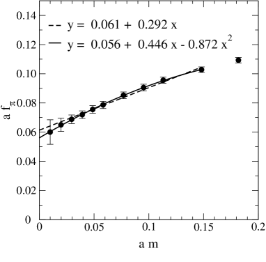
Figure 9: Results for $f_{\pi}$ for $D_{CI}$, $16^{3}\times 32$, $\beta_{LW}=8.7$, $a=0.08~{}\textrm{fm}$ together with fits linear or quadratic in $a\,m$.

Since the source is typically smeared, we measured propagators from the smeared source to point sinks and smeared sinks. Appropriate ratios then allow us to recover e.g. unsmeared-unsmeared type propagators.

Fig. 9 shows $f_{\pi}$ as a function of the bare mass for $D_{CI}$ comparing a linear and a quadratic fit. For the extrapolation to the chiral limit we use the results from the quadratic fit. The chiral extrapolations of $af_{\pi}$ in Figs. 10 and 11 show excellent scaling behaviour.

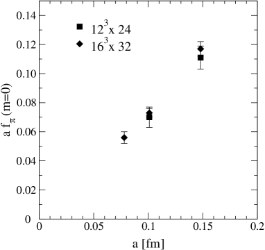
Figure 10: The (quadratic) extrapolations of $f_{\pi}$ to the chiral limit for different lattice spacings exhibit simple scaling behaviour (results for $D_{CI}$).

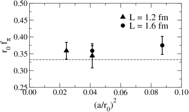
Figure 11: The (quadratic) extrapolations of $f_{\pi}$ to the chiral limit for different lattice spacings in dimensionless units ($r_{0}$ denotes the Sommer parameter) exhibit simple scaling behaviour (results for $D_{CI}$). The dashed line corresponds to the experimental (i.e. unquenched) value 131 MeV.

4 Light hadron spectroscopy

The parameters of our simulations (Table 1) allow us to make a scaling study with both actions in a fixed volume $L\approx 1.3$ fm at lattice constants $a\approx 0.08$, $0.10$ and $0.15$ fm and a finite volume analysis at fixed $a\approx 0.15$ fm in boxes with $L=1.3-2.6$ fm. We considered $\sim 10$ different quark masses and inverted the Dirac matrix with a multimass solver. Note that the hadron masses at different quark masses with other parameters fixed are strongly correlated.

With this setup we could study different aspects of light hadron spectroscopy close to the chiral limit. The subject is old, nevertheless we found surprises, results which we do not quite understand and which require further study.

4.1 Hadron spectroscopy in terms of hadronic scales

Since our main interest lies in understanding the behaviour of the Dirac operators, it is natural to fix the scale within the hadronic sector itself. In Sect. 4.3 we shall connect these results to the typical gauge sector scale $r_{0}$ also.

An obvious candidate to carry the scale could be the vector meson mass $m_{V}$ at the quark mass where $m_{PS}/m_{V}$ is equal to the experimental value. Identifying this vector meson mass with $m_{\rho}\approx 770$ MeV gives the cutoff and all the masses in MeV. This choice for the scale has the disadvantage that it refers to the rho mass deep in the chiral limit and is plagued by relatively large statistical errors. For many purposes (like scaling and finite volume studies) it is better to fix the scale by the vector meson mass $m_{V}(x)$, where $m_{PS}/m_{V}=x$ fixed and chosen in a range where $m_{V}(x)$ can be precisely determined. In our analysis we have taken $x=0.75$. A similar method was used earlier in the works [20].

Fig. 12 gives the vector meson mass $m_{V}$ as a function of the pseudoscalar mass $m_{PS}$ in $m_{V}(0.75)$ units. All our simulation results from Table 1 are collected in this figure. Independently of the lattice scale $a$, the size of the box ($L=1.3-2.6$ fm) and for both Dirac operators the points lie on a universal curve. This observation goes beyond our work: collecting data from other large scale simulations performed with different Dirac operators (Wilson, clover, staggered fermions with or without improvement) the results lie on this curve [27]. The point (0.75,1) of this curve is fixed by definition; the other points seem to be then independent of the cut-off in the range of recent simulations and in volumes down to $L\approx 1.3$ fm.

Fig. 13 shows the nucleon mass as a function of $m_{PS}$ in $m_{V}(0.75)$ units for the FP Dirac operator. The points forming the upper curve all refer to $L\approx 1.3$ fm, they represent a scaling test for $a\approx(0.08-0.16)$ fm. Within the statistical errors no scaling violation is seen in this figure. The conclusion is the same for the CI operator. The large volume ($L\approx 2.5$ fm) results form the lower curve. These points were obtained on a coarse lattice with $a\approx 0.16$ fm.

For heavy quark masses we expect that the nucleon finite size effects will become smaller. We see indeed in Fig. 13 that the two curves join for heavy quarks. This has an additional message. Since the upper curve scales, we might assume it is close to the continuum limit. This suggests that the large volume curve (for which we do not have a scaling test) is also, at least for heavy quarks, close to the continuum limit.

Fig. 14 illustrates that the scaling of the $D_{FP}$ data in Fig. 13 is not ’built in’ in the quantity studied. In this figure our large volume results are compared with the CP-PACS data from their recently completed analysis [21]. These results were obtained with the Wilson Dirac operator at four different lattice spacings ($a=0.05-0.10$ fm). For the clarity of the figure we plotted the $a=0.05$ fm and $a=0.10$ fm data only. Even the $a=0.05$ fm points are rather far from the continuum as estimated in [21]. The difficulty of such a continuum extrapolation is illustrated in Fig. 16.

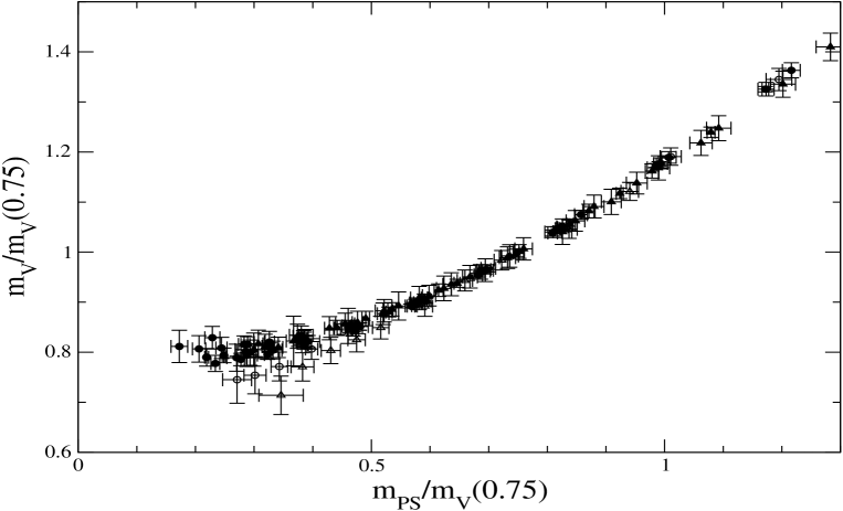
Figure 12: All the results on the vector and pseudoscalar masses of our simulations with different lattice spacings, volumes and actions. The scale is carried by the vector meson mass where $m_{PS}/m_{V}=0.75$.

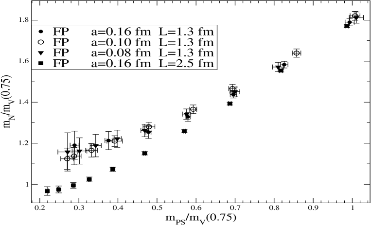
Figure 13: The nucleon mass as a function of the pseudoscalar mass. The upper curve is a scaling test in a fixed volume.

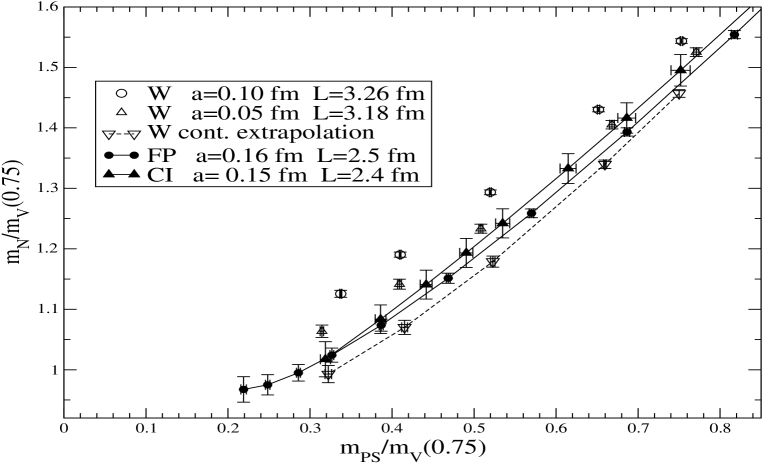
Figure 14: Similar to Fig. 13. The large volume FP and CI results obtained on coarse configurations are compared with Wilson data and their continuum limit extrapolation [21].

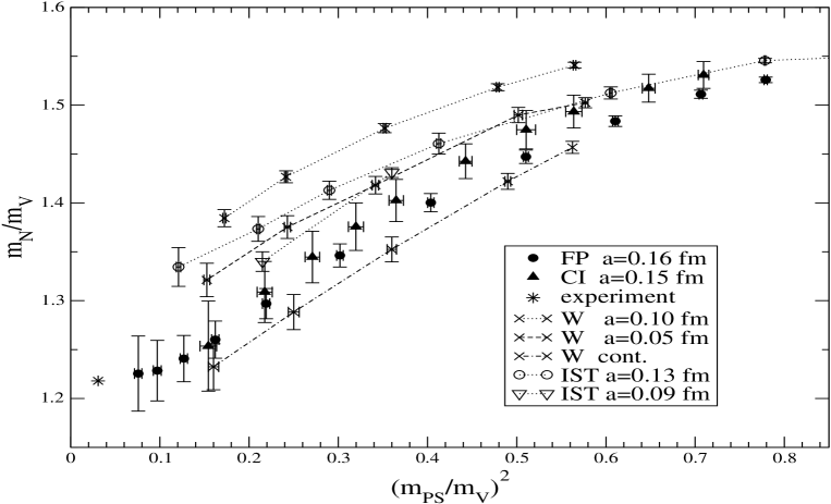
Figure 15: APE plot where the FP and CI results are compared with Wilson [21] and improved staggered data [26].

The four sets of points in Fig. 16 refer to $x=m_{PS}/m_{V}=$ 0.75, 0.7, 0.6 and 0.4. For each set a linear extrapolation is done using the results at 4 different lattice spacings. The data and the extrapolated points at $a=0$ are taken from [21]. The 4 points on the r.h.s. of Fig. 16 are the FP numbers at $a\approx 0.16$ fm for the 4 different $x$-values. Further results are needed to make a firm conclusion from Fig. 14.

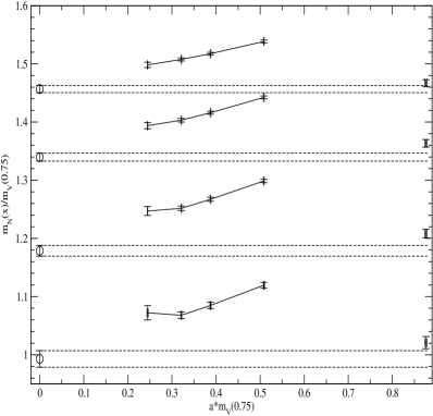
Figure 16: The continuum extrapolation of the CP-PACS Wilson data [21] for 4 different x-values. The points on the far right are the FP $a\approx 0.16$ fm results.

Fig. 15 is a standard APE plot where the large volume, coarse lattice FP $a\approx 0.16$ fm and CI $a\approx 0.15$ fm data are compared with the CP-PACS results [21] and with the improved staggered fermion data obtained at $a=0.13$ fm [26] and $a=0.09$ fm [25] (2 points only). The coarse FP and CI data are significantly closer to the CP-PACS continuum extrapolated curve than the fine lattice Wilson or the improved staggered points. On the other hand, as we remarked above, the long continuum extrapolation of the Wilson data [21] is not an easy task.

4.2 Dispersion relation and the speed of light

Another quantity which can be studied within the hadronic sector is the energy-momentum dispersion relation. As earlier investigations show, $E=E({\vec{p}}\,)$ is a cut-off sensitive quantity and the deviations from the continuum form $(E^{2}({\vec{p}}\,)-m^{2})/{\vec{p}}^{\;2}=c^{2}$ can be large. Here $c$, the speed of light, should be independent of ${\vec{p}}$ and equal to 1 in our convention. For the FP Dirac operator at $a\approx 0.16$ fm in a box with $L\approx 2.5$ fm the energy $E({\vec{p}}\,)$ could be determined with relatively small errors in the momentum range $|{\vec{p}}\,|=(0.5-1.0)$ GeV and the corresponding dispersion relation can not be distinguished from its continuum form [3, 27].

Fig. 17 shows the speed of light as a function of the quark mass for the vector and pseudoscalar meson as measured by the FP and the 3 overlap steps augmented FP Dirac operators. For both hadrons the FP operator results show no deviation from 1, while the data with the overlap augmented operator lie above 1 beyond the statistical errors. We find this result difficult to understand. Starting with the parameterized FP operator which approximates quite well a GW solution, we expected to produce small changes only by performing 3 overlap steps.

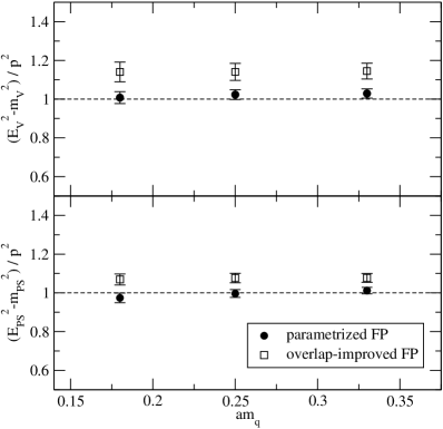
Figure 17: The speed of light as obtained from the vector and pseudoscalar channels as a function of the quark mass.

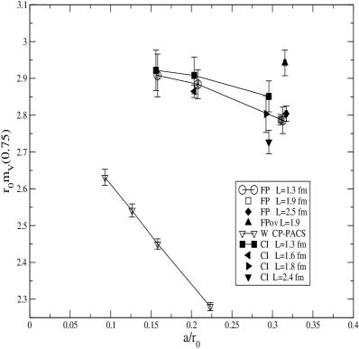
Figure 18: Scaling test for $r_{0}m_{V}(0.75)$.

4.3 Connecting the hadronic and gauge scales

In order to connect the hadron sector with the gauge sector it is sufficient to relate the reference scale $m_{V}(0.75)$ we used above with a gauge theory scale, like $r_{0}$ [22]. The Sommer parameter has been measured for both actions close to the $\beta$- range of our simulations [10, 14].

Fig. 18 shows $r_{0}m_{V}(0.75)$ as a function of the lattice resolution. The 3 FP data on the coarsest lattice with different volumes $L=1.3-2.5$ fm completely coincide showing that $m_{V}(0.75)$ has no finite size effect within the small errors in these boxes. This is consistent with Fig. 12. The 3 CI data on the coarsest lattice are consistent with the FP number, but have larger errors.

Relative to this coarsest point the $a\approx$0.10 and 0.08 fm data lie higher and indicate cut-off effects in $r_{0}m_{V}(0.75)$. We have to remember though that measuring $r_{0}$ on a coarse lattice is a difficult, perhaps not even quite well defined problem.

As Fig. 18 shows, the prediction of the overlap augmented FP Dirac operator on the coarsest lattice is definitely inconsistent with that of the FP result. Since the Dirac operators FP and ov3 were used on the same gauge configurations (therefore they see the same $a$ and $r_{0}$ in a quenched theory) we have to conclude that one or both Dirac operators have clearly identified cut-off effects in $m_{V}(0.75)$ at $a\approx 0.16$ fm. For comparison we also included the Wilson data [21] in Fig.18.

5 Pion scattering length

The pion scattering length is an important observable characterizing dynamical effects of the strong interaction and its ab initio calculation on the lattice is an important nonperturbative test of QCD. In the literature several attempts to compute the scattering length with Wilson fermions [28, 29, 30, 31, 32] and staggered fermions [28, 29] can be found. However, calculations with a chiral Dirac operator which allows for a better control of the small mass region are still missing. In full QCD the scattering length is a quantity which vanishes in the chiral limit, while it is power divergent in the quenched theory [33] and eventually a study in the full theory is desirable. This is the initial stage of our investigation which we regard as a preparation for a simulation in the full theory when unquenched configurations become available. In this preliminary study we reuse the FP propagators computed for the spectroscopy to calculate the $\pi\pi$ S-wave scattering length in the $I=2$ channel. Although using these propagators with only a single source limits the quality of the overlap with the pion scattering state the results are quite encouraging and a more refined investigation is in preparation.

5.1 Method

In order to calculate the $\pi^{+}\pi^{+}$ scattering length from a Euclidean lattice simulation, we use Lüscher’s relation [34] that relates the energy shift of the two pion state, $\Delta E(L)$, in a finite volume ($V=L^{3}$) to the scattering length, $a_{0}$, in the infinite volume limit to order $1/L^{5}$,

$$\Delta E=-\frac{4\pi a_{0}}{m_{\pi}L^{3}}\left\{1+c_{1}\frac{a_{0}}{L}+c_{2}\frac{a_{0}^{2}}{L^{2}}+\cdots\right\}\;,$$ (10)

where $c_{1}=-8.9136$ and $c_{2}=62.9205$ are numerical constants computed in [34]. Propagators generated for the spectroscopy study were used to construct the two pion state and to measure its energy, $E=2\,m_{\pi}+\Delta E$. In other words, a single Gaussian source was used to create the two pions on the gauge fixed configurations. We also applied the same Gaussian smearing at the sinks in this study. We worked on the $8^{3}\times 24$ and $12^{3}\times 24$ lattices at $a=0.16$ fm. All the scattering lengths shown in Fig. 21 are for $m_{\pi}\,L>4$ except for the two lightest masses for $L=12\,a$ where $m_{\pi}\,L$ is only larger than $3$.

5.2 Analysis

We extract the energy shift of the two pion state in a finite volume by considering ratios of two pion correlation functions and single pion correlation functions. We follow the procedure and notation of Ref. [28] and construct the “direct” (D) and “crossed” (C) contractions of

$$\left\langle\sum_{\vec{x}_{1}}{\mathcal{O}}_{1}(\vec{x}_{1},t)\sum_{\vec{x}_{2}}{\mathcal{O}}_{2}(\vec{x}_{2},t){\mathcal{S}}(t=0){\mathcal{S}}(t=0)\right\rangle\;,$$ (11)

where ${\mathcal{O}}$ annihilates a $\pi^{+}$ and ${\mathcal{S}}$ are the gaussian sources for the pions. Note that D and C actually refer to the ratio after dividing by two single pion correlators. In practice we fit the numerator and denominator separately. The different diagrams (contractions) of ratios are labeled,

$D(t)\sim$ glue exchange between the two pions
$C(t)\sim$ quark exchange between the two pions

where the combination of interest ($I=2$) is $D(t)-C(t)$ whose large $t$ behaviour is approximately $Ze^{-\Delta Et}$. We have also expanded the exponential to leading order in $\Delta Et$ in the fit, but there were no differences within the errors.

Periodic boundary conditions were used in the time direction so that we must take into account a backwards propagating pion. The fitting form of the two-particle correlator (the numerator of $D(t)-C(t)$) is

$$Z_{\pi\pi}(e^{-(2m_{\pi}+\Delta E)t}+e^{-(2m_{\pi}+\Delta E)(T-t)}+ze^{-m_{\pi}T})\;.$$ (12)

We simultaneously fit the pion propagator entering the denominator for $Z_{\pi}$ and $m_{\pi}$,

$$Z_{\pi}(e^{-m_{\pi}t}+e^{-m_{\pi}(T-t)})\;,$$ (13)

resulting in the following five fitting parameters: $m_{\pi},Z_{\pi},\Delta E,Z_{\pi\pi}$ and $z$. We perform a fully correlated fit to the two correlation functions. In the two figures that follow, we show the fits for the following set of parameters,

$\beta_{FP}=3.00$, $a\approx 0.16$ fm

$N_{s}=12$, $N_{t}=T=24$

$m_{\pi}/m_{\rho}=0.41$, $200$ configurations

which is representative of all the other fits.

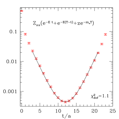
Figure 19: The numerator of the $D-C$ function.

In Fig. 20, we show how the extracted $a_{0}$ depends on the initial time slice included in the fit. We see that nearly any time slice from $t=2\,a$ gives the same results (with reasonable $\chi^{2}$ values) within the errors. This may be somewhat surprising considering that our two pion sources are on top of each other. We take the value for the fit starting at $t_{min}=3\,a$ in this particular case. There were substantial difficulties in getting results for the other lattice spacings as the temporal extent of the box was not as long and/or short of statistics. In the following, we mainly discuss the results from the lattice described above.

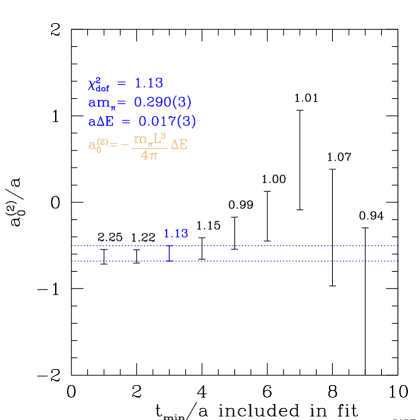
Figure 20: Fit results for $a_{0}$ vs $t_{min}$. The dashed lines mark the value chosen.

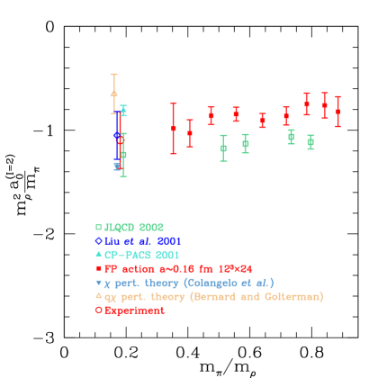
Figure 21: Summary of our results and other recent calculations.

5.3 Results and discussion

Using the parameterized fixed-point action, we have extracted the $\pi^{+}\pi^{+}$ S-wave scattering length at threshold with the propagators generated for spectroscopy studies. We were able to obtain results for the $\beta_{FP}=3.0,12^{3}\times 24$ lattice and for some of the larger masses on the $8^{3}\times 24$ lattice. In Fig. 21, we plot the dimensionless quantity (as was used in Ref. [31]), $m_{\rho}^{2}a_{0}/m_{\pi}$, against $m_{\pi}/m_{\rho}$. We also include in this plot some recent results from other groups as well as quenched chiral perturbation theory [33] and chiral perturbation theory predictions [35]. Our raw results on a coarse lattice are in reasonable agreement with Wilson/clover action results on finer lattices or continuum limit extrapolated numbers. Since we mostly only have results from a single coupling, no real scaling tests could be performed for $a_{0}$.

However, agreement between two of the coarser lattices in limited cases for $m_{\pi}L>4$ and $m_{\pi}/m_{\rho}$ ratios larger than $0.6$ indicate that they are small (also found in spectroscopy studies). The difficulties of extracting the numbers from the other lattices are likely due to contamination from higher momentum pion states. These effects can be reduced by introducing another source, which is currently under study. As remarked above some zero mode effects were observed in the pseudoscalar propagator in the spectroscopy study for $m_{PS}/m_{V}$ mass ratios less than $0.5$. These finite size effects as well as other systematic error studies are work in progress.

6 Summary and conclusions

We have reported here several calculations of quantities relevant for light quark phenomenology using two different Dirac operators which are approximate solutions of the Ginsparg-Wilson equation.

Both actions, beyond having good chiral behaviour, exhibited significantly smaller cut-off effects at $a\sim 0.15$ fm than the standard Wilson action at $a\sim 0.05$ fm and the improved-staggered action at $a\sim 0.09$ fm on hadronic quantities that we have surveyed.

We believe that the improvement more than compensates the apparent increase in the cost of simulating our operators and that a study of dynamical simulations with these actions is a relevant challenge for the future.

Acknowledgements: The calculations were done on the Hitachi SR8000 at the Leibniz Rechenzentrum in Munich and at the Swiss Center for Scientific Computing in Manno. We thank the LRZ staff for training and support. This work was supported in parts by DFG, BMBF and SNF and by the European Community’s Human Potential Programme under contract HPRN-CT-2000-00145. C. Gattringer acknowledges support by the Austrian Academy of Sciences (APART 654).

References

- [1] P. Hasenfratz, F. Niedermayer, Nucl. Phys. B 414 (1994) 785.
- [2] P. Hasenfratz, S. Hauswirth, K. Holland, T. Jörg, F. Niedermayer and U. Wenger, Int. J. Mod. Phys. C 12 (2001) 691.
- [3] S. Hauswirth, Light hadron spectroscopy in quenched lattice QCD with chiral fixed-point fermions, Thesis, Bern University 2002, hep-lat/0204015; T. Jörg, Chiral measurements in quenched lattice QCD with fixed-point fermions, Thesis, Bern University 2002, hep-lat/0206025.
- [4] P. Hasenfratz, S. Hauswirth, T. Jörg, F. Niedermayer and K. Holland, hep-lat/0205010.
- [5] C. Gattringer, Phys. Rev. D 63 (2001) 114501.
- [6] C. Gattringer, I. Hip, C.B. Lang, Nucl. Phys. B 597 (2001) 451.
- [7] P. Ginsparg, K.G. Wilson, Phys. Rev. D 25 (1982) 2649.
- [8] L. Giusti, Exact chiral symmetry on the lattice: QCD applications, plenary talk at Lattice’ 02, these proceedings.
- [9] C. Gattringer, these proceedings, hep-lat/0208056.
- [10] F. Niedermayer, P. Rüfenacht and U. Wenger, Nucl. Phys. B 597 (2001) 413.
- [11] R. Narayanan and H. Neuberger, Phys. Lett. B 302 (1993) 62, Nucl. Phys. B 443 (1995) 305.
- [12] M. Lüscher and P. Weisz, Commun. Math. Phys. 97 (1985) 59; Err.: 98 (1985) 433; G. Curci, P. Menotti and G. Paffuti, Phys. Lett. B 130 (1983) 205, Err.: B 135 (1984) 516.
- [13] A. Hasenfratz and F. Knechtli, Phys. Rev. D 64 (2001) 034504.
- [14] C. Gattringer, R. Hoffmann and S. Schaefer, Phys. Rev. D 65 (2002) 094503.
- [15] C. Best, M. Göckeler, R. Horsley, E.M. Ilgenfritz, H. Perlt, P.E.L. Rakow, A. Schäfer, G. Schierholz, A. Schiller and S. Schramm Phys. Rev. D 56 (1997) 2743; C. R. Allton et al. (UKQCD Collaboration), Phys. Rev. D 47 (1993) 5128.
- [16] T. Blum et al., hep-lat/0007038;
- [17] S.J. Dong, T. Draper, I. Horváth, F.X. Lee, K.F. Liu and J.B. Zhang, Phys. Rev. D 65 (2002) 054507.
- [18] S.R. Sharpe, Phys. Rev. D 46 (1992) 3146; C.W. Bernard and M.F.L. Golterman, Phys. Rev. D 46 (1992) 853.
- [19] T. W. Chiu and T. H. Hsieh, Phys. Rev. D 66 (2002) 014506; T. Draper, S.J. Dong, I. Horváth, F.X. Lee, K.F. Liu, N. Mathur and J.B. Zhang, hep-lat/0208045.
- [20] C. R. Allton et al., Nucl. Phys. B 489 (1997) 427; L. Giusti, C. Hoelbling and C. Rebbi, Phys. Rev. D 64 (2001) 11450.
- [21] S. Aoki et al. (CP-PACS collaboration), hep-lat/0206009.
- [22] R. Sommer, Nucl. Phys. B 411 (1994) 839. ALPHA, M. Guagnelli, R. Sommer and H. Wittig, Nucl. Phys. B 535 (1998) 389.
- [23] L. Giusti, C. Hoelbling, and C. Rebbi, Phys. Rev. D 64 (2001) 114508; Err. ibid. D65 (2002) 079903.
- [24] Y. Kikukawa and A. Yamada, hep-lat/9810024.
- [25] D. Toussaint et al., Nucl. Phys. B (Proc. Suppl.) 106 (2002) 111.
- [26] C. Bernard et al., Phys. Rev. D 64 (2001) 054506.
- [27] BGR Collaboration, in preparation.
- [28] S.R. Sharpe, R. Gupta and G.W. Kilcup, Nucl. Phys. B 383 (1992) 309.
- [29] M. Fukugita, Y. Kuramashi, M. Okawa, H. Mino and A. Ukawa, Phys. Rev. D 52 (1995) 3003.
- [30] CP-PACS Collaboration, Nucl. Phys. B (Proc. Suppl.) 106 (2002) 230.
- [31] C. Liu, J. Zhang, Y. Chen and J.P. Ma, Nucl. Phys. B 624 (2002) 360.
- [32] JLQCD Collaboration, hep-lat/0206011.
- [33] C. Bernard and M. Golterman, Phys. Rev. D 53 (1996) 476.
- [34] M. Lüscher, Nucl. Phys. B 354 (1991) 531.
- [35] G. Colangelo, J. Gasser and H. Leutwyler, Nucl. Phys. B 603 (2001) 125.