Using Approximating Polynomials in Partial-Global Dynamical Simulations

Abstract

Smeared link fermionic actions can be straightforwardly simulated with partial-global updating. The efficiency of this simulation is greatly increased if the fermionic matrix is written as a product of several near-identical terms. Such a break-up can be achieved using polynomial approximations for the fermionic matrix. In this paper we will focus on methods of determining the optimum polynomials.

1 MOTIVATION

Dynamical fermion simulations with smeared links are used more and more frequently. Smeared links improve the chiral and flavor symmetry of Wilson and staggered fermionic actions (see references in [1]). The main obstacle in using these actions is finding efficient algorithms to simulate them. In this paper we present some techniques that are used to improve the efficiency of these simulations. We will focus here on the HYP action [1, 2, 3, 4], but we believe that these methods are more general and can be used for different actions as well.

The HYP action [3] is a modified staggered fermion action

$$S=S_{G}\left(U\right)+\bar{S}_{G}(V)+S_{F}\left(V\right)$$ (1)

where $S_{G}$ is the traditional pure gauge action defined in terms of thin links $U$, $\bar{S}_{G}$ is a gauge action defined in terms of smeared links $V$ and

$$S_{F}=-\frac{n_{f}}{4}\ln\det\Omega,$$ (2)

where $\Omega=M^{\dagger}M$ restricted to even sites, is the staggered fermion action defined in terms of HYP links $V$ rather than thin links. The role of $\bar{S}_{G}$ is discussed in [3].

To simulate this action we use a two step approach. We first update a part of the thin links, $U\rightarrow U^{\prime}$, using a heath-bath and/or an over-relaxation step, then we smear the thin links using the hyper-cubic (HYP) blocking [2] and compute the fat link action, $S_{G}\left(V^{\prime}\right)+S_{F}\left(V^{\prime}\right)$. We accept this new configuration with probability

$$P_{acc}=\min\left\{1,e^{-\bar{S}_{G}\left(V^{\prime}\right)+\bar{S}_{G}\left(V\right)-S_{F}\left(V^{\prime}\right)+S_{F}\left(V\right)}\right\}.$$ (3)

The most difficult step in the algorithm is computing the determinant ratio

$$e^{-S_{F}\left(V^{\prime}\right)+S_{F}\left(V\right)}=\left(\frac{\det\Omega\left(V^{\prime}\right)}{\det\Omega\left(V\right)}\right)^{n_{f}/4}$$

$$=\frac{\int d\xi d\xi^{\dagger}e^{-\xi^{\dagger}\left(\Omega^{\prime-1/2}\Omega\Omega^{\prime-1/2}\right)^{n_{f}/4}\xi}}{\int d\xi d\xi^{\dagger}e^{-\xi^{\dagger}\xi}}.$$ (4)

Instead of computing the ratio itself we use a stochastic estimator suggested by the last part of the relation above

$$E_{A}\left[\xi\right]=e^{-\xi^{\dagger}\left(A-1\right)\xi},$$ (5)

where $A=\left(\Omega^{\prime-1/2}\Omega\Omega^{\prime-1/2}\right)^{n_{f}/4}$. This estimator averages to the determinant ratio since $A$ is hermitian and positive definite. Furthermore, the variance of this estimator is

$$\sigma^{2}\left(E_{A}\right)=\frac{1}{\det\left(2A-1\right)}-\frac{1}{\left(\det A\right)^{2}}.$$ (6)

The relation above holds only if the spectrum of $A$ is bounded from below by 1/2 otherwise the variance diverges. This condition is not necessarily fulfilled by our matrix. To address this problem we modify our stochastic estimator

$$E^{\prime}_{A}\left[\xi\right]=e^{-\sum_{j=1}^{n}\xi_{j}^{\dagger}\left(A^{1/n}-1\right)\xi_{j}}.$$ (7)

This estimator has a finite variance if the lowest eigenvalue of $A$ is greater than $1/2^{n}$. This condition can be fulfilled if we choose $n$ properly. However, this forces us to compute the $n^{th}$ root of fermionic matrices. This is why we are forced to use the polynomial approximation.

In order to make the algorithm more efficient we employed a reduced matrix [2, 3, 4]: $\Omega_{r}=\Omega e^{-2f\left(\Omega\right)}$, where $f$ is a cubic function. The fermionic part will be $S_{F}=\frac{n_{f}}{4}\ln\det\Omega_{r}$ and the reminder is absorbed in $\bar{S}_{G}$.

Lastly, we mention that it can be proved that the algorithm satisfies the detailed balance condition for either of the estimators presented above.

2 POLYNOMIAL APPROXIMATION

To compute the estimator (7), where $A=\left(\Omega_{r}^{\prime-1/2}\Omega_{r}\Omega_{r}^{\prime-1/2}\right)^{n_{f}/4}$, we need to find polynomial approximations for the matrix functions involved in the estimator

$$P^{\left(n\right)}_{k}\left(\Omega\right) \simeq F\left(\Omega\right)^{-1/2n},$$

$$Q^{\left(n\right)}_{k}\left(\Omega\right) \simeq F\left(\Omega\right)^{1/n},$$ (8)

where $F\left(\Omega\right)=\left(\Omega\exp\left[-2f\left(\Omega\right)\right]\right)^{n_{f}/4}$, $n$ is the break-up level and $k$ is the polynomial order.

For a polynomial to approximate a matrix function it needs to approximate the function well on the entire spectrum of the matrix. To determine these polynomials we employed a least square method [5]. The coefficients $t_{i}$ of the polynomial $T$ approximating the function $g$ are determined by minimizing the quadratic “distance”

$$\delta^{2}\left(t_{i}\right)=\int_{\lambda_{0}}^{\lambda_{1}}dx\,\rho(x)\left(T\left(x\right)-g\left(x\right)\right)^{2},$$ (9)

where $\lambda_{0}$, $\lambda_{1}$ are the spectral bounds of $\Omega$ and $\rho$ is a weight function, ideally $\Omega$’s spectral density.

This method has the advantage that it turns into a linear problem and the solution is

$$t_{i}=\sum_{j=0}^{k}\left(K^{-1}\right)_{ij}g_{j},$$ (10)

where $k$ is the polynomial order and

$$K_{ij} = \int_{\lambda_{0}}^{\lambda_{1}}dx\,\rho\left(x\right)x^{i+j},$$

$$g_{i} = \int_{\lambda_{0}}^{\lambda_{1}}dx\,\rho\left(x\right)x^{i}g\left(x\right).$$ (11)

For our polynomials we used $\lambda_{0}=4m^{2}$, the lowest eigenvalue for the staggered fermions matrix. We set the upper bound to $\lambda_{1}=16.4$ which we found to be a good limit for the range of parameters we used in our simulations. It should be mentioned that the only hard upper bound for the spectrum of $\Omega$ is $64+4m^{2}$ but this limit is reduced dynamically. The smearing reduces the value of the highest eigenvalue even further.

The weight function $\rho\left(x\right)$ should approximate the spectral density for $\Omega$. However, we found that for reasonable weight functions the coefficients depend very little on the detailed form. Thus, we used a weight function of the form $\rho\left(x\right)=x^{\alpha}$ which is more convenient for our computation. The advantage of this form is that we can compute the $K_{ij}$ matrix analytically and also it generates a recursion relation for the coefficients $g_{i}$.

To measure the accuracy of the approximation we used the distance function (9) where we set $\rho\left(x\right)=1$. In Fig.1 we plot the distance between $\left[P^{\left(n\right)}\right]^{2n}$, $\left[Q^{\left(n\right)}\right]^{n}$ and $F\left(x\right)^{\mp 1}$ as a function of the polynomial order. We notice first that $Q^{\left(1\right)}$ is a much better approximation than $Q^{\left(n\right)}$ for $n>1$. This is due to the fact that $F\left(x\right)$ (which is the function that $Q^{\left(1\right)}$ approximates) has an almost polynomial behavior close to $\lambda_{0}$ where the function is the hardest to approximate. Another interesting feature that we notice in the graphs is that the order of the approximation doesn’t improve with increasing break-up level. This is puzzling, at first, since as $n$ increases the equivalent order of the polynomial approximating $F\left(x\right)^{\pm 1}$ is $n\times k$. However, the number of variables varied to minimize $\delta$ stays the same and it seems that this is the determining factor for the order of approximation.

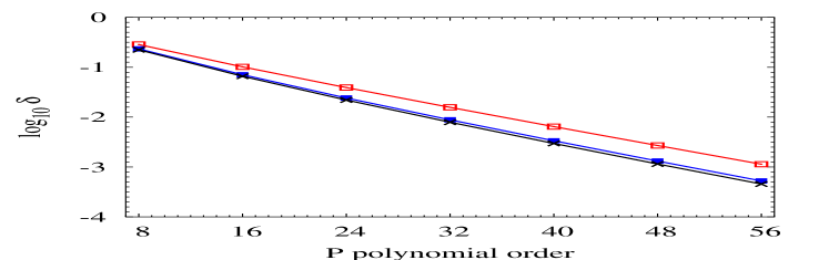
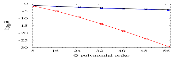
Figure 1: The accuracy level for the P and Q polynomials: open squares $n=1$, filled squares $n=4,$ crosses $n=8$ ($am=0.10$).

We found that when $\delta\sim 10^{-8}$ the numerical roundoff error becomes dominant and the higher order polynomials do not improve the precision of the calculation. Thus, we will be using the polynomials with $\delta\sim 10^{-8}$ as “exact” ones. We see in Fig. 1 that these polynomials have an order of $k\sim 100$. The only exceptions are the polynomials for $n=1$ but they are of no real interest since they don’t satisfy the minimum eigenvalue requirement.

To further reduce the cost of computing the estimator we implemented a two step approach. Since we only use the value of the estimator in the accept reject step we only need to know whether the value of the estimator is larger or smaller that $\ln r$, where $r$ is the random number. We will first compute the estimator approximatively, using small order polynomials; if the distance between the approximate value and $\ln r$ is greater than $\epsilon$ we use this value in the accept reject step. If not, we “fall-back”, i.e. we compute the “exact” value of the estimator using the large polynomials. The value of $\epsilon$ is determined in a small run as the maximum difference between the approximate estimator and its “exact” value. The rate of fall-back is usually around 10% and this reduces the computational cost substantially. Having fixed the large polynomials by the $\delta$ condition we determine the optimum small ones that minimize the computational cost. The cost is given by the number of $M^{\dagger}M$ multiplies and it is determined by the order of the polynomials used. We found that the order of the optimum small polynomial is independent of the break-up level (see Fig.2) and it increases as we decrease the mass. We find that for $am=0.10$ we need $k=24$, for $am=0.06$ $k=32$ and for $am=0.04$ $k=48$.

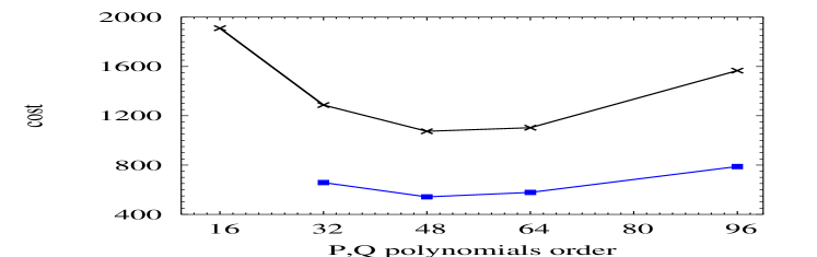
Figure 2: Cost vs the polynomial order for $m=0.04$ and $n=4,8$.

3 CONCLUSIONS

We have showed how to use the polynomial approximation for simulating dynamical fermions. First we determine the minimum break-up level $n$ using the minimum eigenvalue requirement. Then we determine the large polynomials using the $\delta\sim 10^{-8}$ conditions. We then determine the optimum small polynomials using the minimum cost condition. For a more complete discussion see [4].

References

- [1] A. Hasenfratz, plenary talk at Lattice 2002.
- [2] A. Hasenfratz, F. Knechtli, Phys. Rev. D 64 (2001) 034504.
- [3] A. Hasenfratz, A. Alexandru, Phys. Rev. D. 65 (2002) 114506.
- [4] A. Alexandru, A. Hasenfratz, hep-lat/0207014.
- [5] I. Montvay, Comput. Phys. Commun. 109 (1998) 144.