Improving the Partial-Global Stochastic Metropolis Update for Dynamical Smeared Link Fermions

Abstract

We discuss several methods that improve the partial-global stochastic Metropolis (PGSM) algorithm for smeared link staggered fermions. We present autocorrelation time measurements and argue that this update is feasible even on reasonably large lattices.

Smeared link actions have gained popularity in recent years. These actions have many desirable features: improved flavor symmetry with staggered fermions, smaller perturbative matching factors, better topology, etc [1]. What hinders the use of these smeared actions is the difficulty of dynamical simulations with standard molecular dynamics type algorithms. Recently it was suggested that even projected smeared link actions can be effectively simulated with partial-global heatbath or over-relaxation updates that are combined with a Metropolis type accept-reject step [2]. In this paper we summarize some of the improvements that make this partial-global stochastic Metropolis (PGSM) update truly effective.

1 THE SMEARED LINK ACTION AND THE PARTIAL-GLOBAL UPDATE

We consider a smeared link action of the form

$$S=S_{g}(U)+\bar{S}_{g}(V)+S_{f}(V),$$ (1)

where $S_{g}(U)$ and $\bar{S}_{g}(V)$ are gauge actions depending on the thin links $\{U\}$ and smeared links $\{V\}$, respectively, and $S_{f}$ is the fermionic action depending on the smeared links only. The smeared links are constructed deterministically. Here we use HYP blocking [3]. $S_{g}(U)$ is an arbitrary gauge action, and $\bar{S}_{g}(V)$ contains 4 and 6-link loops of the smeared links. We choose the coefficients of $\bar{S}_{g}(V)$ to improve computational efficiency. The fermionic action describing $n_{f}$ degenerate flavors with staggered fermions is $S_{f}(V)=-\frac{n_{f}}{4}\ln\,\mathop{\hbox{det}}\,\Omega(V)$ with $\Omega(V)=(M^{\dagger}(V)M(V))$ defined on even sites only.

We use the partial-global stochastic updating (PGSM) algorithm to simulate this system [2]. The PGSM algorithm is a variation of the pseudo-fermion method and satisfies the detailed balance equation. First a subset of the thin links $\{U\}$ are updated and a new thin gauge link configuration $\{U^{\prime}\}$ is proposed such that the transition probability $p(U,U^{\prime})$ of the update satisfies detailed balance with $S_{g}(U)$ . The proposed configuration is accepted with the probability

$$P_{\rm{acc}}=\rm{min}\{1,e^{-\Delta\bar{S}_{g}}e^{-\xi^{*}[A^{n_{f}/4}-1]\xi}\},$$ (2)

where $\Delta\bar{S}_{g}=\bar{S}_{g}(V^{\prime})-\bar{S}_{g}(V)$, the matrix $A=\Omega^{{}^{\prime}-1/2}\Omega\Omega^{{}^{\prime}-1/2}$, and the stochastic vector $\xi$ is generated with Gaussian distribution, $\rm{exp}(-\xi^{*}\xi)$.

2 IMPROVING THE PGSM UPDATE

The PGSM algorithm averages the stochastic estimator of the fermionic determinant together with the gauge configuration ensemble average and it can be efficient only if the standard deviation of the stochastic estimator is small. The standard deviation of $\mathop{\hbox{det}}A^{-1}$ can be written as

$$\sigma_{A}^{2} = <e^{-2\xi^{*}[A-1]\xi}>-<e^{-\xi^{*}[A-1]\xi}>^{2}$$

$$= \mathop{\hbox{det}}(2A-1)^{-1}-\mathop{\hbox{det}}(A)^{-2}.$$

$\sigma_{A}$ diverges if even one of the eigenvalues of $A$ is less than 1/2, which is likely to occur if $\Omega$ and $\Omega^{\prime}$ differ significantly [4]. We consider two separate methods to solve this problem.

1. Reduction: The fermionic matrix reduction [2, 4] removes the most UV part of the fermionic operator by defining a reduced matrix $\Omega_{r}=\Omega e^{-2f(\Omega)}$ and rewriting the fermionic action as

$$S_{f}(V)=-\frac{n_{f}}{4}\Big{(}\ln\,\mathop{\hbox{det}}\,\Omega_{r}(V)+2\mathop{\hbox{Tr}}f(\Omega)\Big{)}.$$ (3)

If the function $f$ is a polynomial of $\Omega$, $\mathop{\hbox{Tr}}f(\Omega)$ can be evaluated exactly and only the determinant of the reduced matrix $\Omega_{r}$ has to be calculated stochastically. The parameters of $f$ are chosen such as to minimize the eigenvalue spread of $\Omega_{r}$. With $f$ a cubic polynomial the conditioning number of the fermionic matrix can be reduced by about a factor of 30.

2. Determinant breakup: Writing the fermionic determinant in the form $\mathop{\hbox{det}}A^{-1}=(\mathop{\hbox{det}}A^{1/n_{b}})^{-n_{b}}$ suggests that the stochastic part of the estimator can be evaluated using $n_{b}n_{f}/4$ independent Gaussian vectors with the replacement

$$e^{-\xi^{*}(A^{n_{f}/4}-1)\xi}\to e^{-\sum^{n_{b}n_{f}/4}_{i=1}\xi_{i}^{*}[A^{1/n_{b}}-1]\xi_{i}}.$$ (4)

The standard deviation of the stochastic estimator is now finite as long as the matrix $\Omega_{r}^{-1/2}(V^{\prime})\Omega_{r}(V)\Omega_{r}^{-1/2}(V^{\prime})$ has no eigenvalue smaller than $1/2^{n_{b}}$, a condition that can always be satisfied [4].

The effectiveness of the fermionic reduction and determinant breakup is illustrated in figure 1 where we show the stochastic estimator on a specific $A$ matrix using no improvement, with fermionic reduction but no determinant breakup, and with fermionic reduction and $n_{b}=8$ determinant breakup. Observe the 16 orders of magnitude difference between between figure 1a and 1c.

Figure 1: The stochastic estimator on a given fermionic matrix $A$ with a) no improvement; b) fermionic reduction but no determinant breakup; c) fermionic reduction and $n_{b}=8$ determinant breakup.

3 TUNING THE ACTION PARAMETERS

Improving the stochastic estimator ensures that the acceptance rate of the PGSM update is close to the theoretical maximum, the exact ratio of the determinants. But the acceptance rate will be large only if the exact ratio is large. That will be the case if the configurations proposed by the pure gauge action $S_{g}(U)$ are close to the dynamical configurations. Chosing $S_{g}(U)$ such that it matches the lattice spacing and/or short distance fluctuations of the expected dynamical configurations can maximize the acceptance rate. Such a matching requires the shift of the pure gauge coupling towards the appropriate quenched value. This shift can be compensated by the $\bar{S}_{g}(V)$ term. $\bar{S}_{g}(V)$ is taken into account in the accept-reject step but since it depends on the smeared links only, it fluctuate much less than $S_{g}(U)$ and does not affect the acceptance rate significantly [5].

4 THE EFFECTIVENESS OF THE PGSM UPDATE

The effectiveness of the PGSM algorithm depends on both the partial-global heat bath update and the stochastic estimator. The autocorrelation time of the simulation is the larger of the autocorrelation times of the heat bath and stochastic steps. We have measured the integrated autocorrelation time of the plaquette as the function of the number of links updated at one heat bath step, $t_{HB}$ [5]. The autocorrelation time of the pure gauge partial-global heat bath update can be expressed as

$$\tau_{pg}=\tau_{HB}\frac{4V}{t_{HB}r_{a}},$$ (5)

where $\tau_{HB}$ is the autocorrelation time of the pure gauge heat bath update, $V$ is the volume of the lattice, and $r_{a}$ is the acceptance rate.

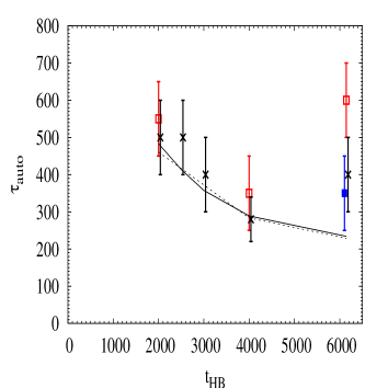
Figure 2: Autocorrelation of the $n_{f}=2$ runs. Open squares: $n_{b}=8$, $am=0.10$, filled squares: $n_{b}=12$, $am=0.10,$ crosses: $n_{b}=12$, $am=0.04$ runs. The lines corresponds to the expected autocorrelation based on the heatbath update alone.

All our simulations were carried out on $8^{3}\times 24$ lattices at lattice spacing $a\sim 0.17$ fm with $n_{f}=2$ fermion flavors. We considered two quark mass values, $am=0.10$ where $m_{\pi}/m_{\rho}\sim 0.71$, and $am=0.04$ where $m_{\pi}/m_{\rho}\sim 0.54$. In figure 2 we plot $\tau_{\rm{auto}}$ for the different runs showing the dependence on the quark mass, determinant breakup, and $t_{HB}$.

We conclude this paper by translating the autocorrelation time measurements to computer time requirements. In figure 3 we plot the computer time measured in fermionic matrix $M^{\dagger}M$ multiplies to create configurations that are separated by $2\tau_{\rm{auto}}$ update steps. Using thin link fermions with standard small step size algorithms, it takes about $8\times 10^{5}$ $M^{\dagger}M$ multiplies to create independent configurations with $am=0.10$. On these 10 fm⁴ lattices it is actually faster to create HYP smeared configurations with PGSM than thin link ones with a small step size algorithm.

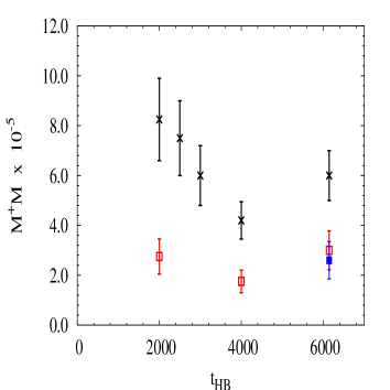
Figure 3: Cost of creating independent configurations, measured in fermionic matrix multiplies. Notation is the same as in figure 2.

The PGSM algorithm scales with the square of the lattice volume. To repeat the above measurements on 100 fm⁴ lattices would increase the computer time by 100. A factor of 10 increase is due to the increased volume, and the other factor of 10 is due to the increased autocorrelation time. Even on 100 fm⁴ volume the PGSM simulation with $am=0.10$ will be only a few times slower than thin link fermion simulations. Simulation cost at smaller lattice spacing but same physical volume increases only linearly with the lattice volume as the number of links that can be effectively touched increases accordingly.

References

- [1] For a review, see A. Hasenfratz, these proceedings.
- [2] A. Hasenfratz and F. Knechtli, Comput. Phys. Commun. 148 (2002) 81.
- [3] A. Hasenfratz, F. Knechtli, Phys. Rev. D64 (2001) 034504.
- [4] A. Hasenfratz, A. Alexandru, Phys. Rev. D65 (2002) 114506.
- [5] A. Alexandru and A. Hasenfratz, arXiv:hep-lat/0207014.