Staggered Fermion Thermodynamics using Anisotropic Lattices

Abstract

Numerical simulations of full QCD on anisotropic lattices provide a convenient way to study QCD thermodynamics with fixed physics scales and reduced lattice spacing errors. We report results from calculations with 2-flavors of dynamical fermions where all bare parameters and hence the physics scales are kept constant while the temperature is changed in small steps by varying only the number of the time slices. The results from a series of zero-temperature scale setting simulations are used to determine the Karsch coefficients and the equation of state at finite temperatures.

1 INTRODUCTION

The anisotropic formulation of lattice QCD has certain advantages when it comes to the study of the equation of state (EOS) at various finite temperatures. The finite temperature field theory has a natural asymmetry which makes the anisotropic approach useful to reduce the lattice spacing errors associated with the transfer matrix at less cost than is required for the full continuum limit[1]. Through the introduction of anisotropy on the lattice one can make the temporal lattice spacing, $a_{t}$, sufficiently small so that by varying only the number of time slices, $N_{t}$, the temperature can be changed in small discrete steps.

Our simulations of full QCD with two flavors of staggered fermions on anisotropic lattices are aimed at the study of the thermodynamic properties of the quark-gluon system. We employ a fixed parameter scheme in which all the bare parameters of the simulation are kept constant and only the temperature is changed by varying $N_{t}$ (from 4 to 64). This approach separates temperature and lattice spacing effects and keeps the underlying physics scales fixed.

The calculation of the EOS of the quark-gluon system involves derivatives of the bare parameters with respect to the physical anisotropy $\xi=a_{s}/a_{t}$ and the spatial lattice spacing $a_{s}$. These “Karsch” coefficients[2] are determined as a by-product of the zero-temperature calculations needed to choose the bare parameters. Once determined, the Karsch coefficients can be used for all temperatures since they depend only on the intrinsic lattice parameters and not on $N_{t}$. This allows a straight-forward determination of the temperature dependence of the energy and pressure, again at fixed lattice spacing. With two or more slightly different values for $a_{t}$, a high-resolution sampling of temperatures can be investigated.

2 THE ANISOTROPIC STAGGERED ACTION AND EOS DERIVATION

Our calculations are based on the QCD action $S^{\xi}=S_{G}^{\xi}+S_{F}^{\xi}$, where the gauge action is:

$$S_{G}^{\xi}=-\frac{\beta}{N_{c}}\frac{1}{\xi_{o}}\left[\sum_{x,s>s^{\prime}}P_{ss^{\prime}}(x)+\xi_{o}^{2}\sum_{x,s}P_{st}(x)\right],$$

and the fermion action is:

$$S_{F}^{\xi} = \sum_{x}\overline{\psi}(x)\left[m_{f}+\nu_{t}\mathchoice{\ooalign{$\hfil\displaystyle\mkern 1.0mu/\hfil$\crcr$\displaystyle D$}}{\ooalign{$\hfil\textstyle\mkern 1.0mu/\hfil$\crcr$\textstyle D$}}{\ooalign{$\hfil\scriptstyle\mkern 1.0mu/\hfil$\crcr$\scriptstyle D$}}{\ooalign{$\hfil\scriptscriptstyle\mkern 1.0mu/\hfil$\crcr$\scriptscriptstyle D$}}^{\rm Staggered}_{t}\right]\psi(x)$$ (18)

$$+\sum_{x}\overline{\psi}(x)\left[\frac{1}{\xi_{0}}\sum_{s}\mathchoice{\ooalign{$\hfil\displaystyle\mkern 1.0mu/\hfil$\crcr$\displaystyle D$}}{\ooalign{$\hfil\textstyle\mkern 1.0mu/\hfil$\crcr$\textstyle D$}}{\ooalign{$\hfil\scriptstyle\mkern 1.0mu/\hfil$\crcr$\scriptstyle D$}}{\ooalign{$\hfil\scriptscriptstyle\mkern 1.0mu/\hfil$\crcr$\scriptscriptstyle D$}}^{\rm Staggered}_{s}\right]\psi(x).$$

To derive the EOS we start from the thermodynamics identities $\varepsilon(T)=-\frac{1}{V_{s}}\left.\frac{\partial\ln Z}{\partial(1/T)}\right|_{V_{s}}$ and $p(T)=T\left.\frac{\partial\ln Z}{\partial V_{s}}\right|_{T}.$

Using the explicit form for $Z$ and changing the independent variables with respect to which we differentiate to $\xi$ and $a_{s}$ we get:

$$\varepsilon(T) = \frac{\xi}{N_{s}^{3}N_{t}a_{s}^{3}a_{t}}\frac{1}{N_{c}}\times$$ (35)

$$\left[\left(\frac{1}{\xi_{o}}\left.\frac{\partial\beta}{\partial\xi}\right|_{a_{s}}+\beta\left.\frac{\partial\xi_{o}^{-1}}{\partial\xi}\right|_{a_{s}}\right)\langle\sum_{x,s>s\prime}{\rm Re}{\rm Tr}\left[P_{ss\prime}(x)\right]\rangle\right.$$

$$\left.+\left(\xi_{o}\left.\frac{\partial\beta}{\partial\xi}\right|_{a_{s}}+\beta\left.\frac{\partial\xi_{o}}{\partial\xi}\right|_{a_{s}}\right)\langle\sum_{x,s}{\rm Re}{\rm Tr}\left[P_{st}(x)\right]\rangle\right]$$

$$+\frac{\xi N_{f}}{4N_{s}^{3}N_{t}a_{s}^{3}a_{t}}\left[\left.\frac{\partial m_{f}}{\partial\xi}\right|_{a_{s}}\langle{\rm Tr}\left[\frac{1}{M}\right]\rangle\right.$$

$$\left.+\left.\frac{\partial\nu_{t}}{\partial\xi}\right|_{a_{s}}\langle{\rm Tr}\left[\frac{\mathchoice{\ooalign{$\hfil\displaystyle\mkern 1.0mu/\hfil$\crcr$\displaystyle D$}}{\ooalign{$\hfil\textstyle\mkern 1.0mu/\hfil$\crcr$\textstyle D$}}{\ooalign{$\hfil\scriptstyle\mkern 1.0mu/\hfil$\crcr$\scriptstyle D$}}{\ooalign{$\hfil\scriptscriptstyle\mkern 1.0mu/\hfil$\crcr$\scriptscriptstyle D$}}_{t}}{M}\right]\rangle\right.+\left.\left.\frac{\partial\xi_{o}^{-1}}{\partial\xi}\right|_{a_{s}}\langle{\rm Tr}\left[\frac{\mathchoice{\ooalign{$\hfil\displaystyle\mkern 1.0mu/\hfil$\crcr$\displaystyle D$}}{\ooalign{$\hfil\textstyle\mkern 1.0mu/\hfil$\crcr$\textstyle D$}}{\ooalign{$\hfil\scriptstyle\mkern 1.0mu/\hfil$\crcr$\scriptstyle D$}}{\ooalign{$\hfil\scriptscriptstyle\mkern 1.0mu/\hfil$\crcr$\scriptscriptstyle D$}}_{s}}{M}\right]\rangle\right]$$

$$p(T) = \frac{\varepsilon(T)}{3}+\frac{a_{s}}{3N_{s}^{3}N_{t}a_{s}^{3}a_{t}}\frac{1}{N_{c}}\times$$ (52)

$$\left[\left(\frac{1}{\xi_{o}}\left.\frac{\partial\beta}{\partial a_{s}}\right|_{\xi}+\beta\left.\frac{\partial\xi_{o}^{-1}}{\partial a_{s}}\right|_{\xi}\right)\langle\sum_{x,s>s\prime}{\rm Re}{\rm Tr}\left[P_{ss\prime}(x)\right]\rangle\right.$$

$$+\left.\left(\xi_{o}\left.\frac{\partial\beta}{\partial a_{s}}\right|_{\xi}+\beta\left.\frac{\partial\xi_{o}}{\partial a_{s}}\right|_{\xi}\right)\langle\sum_{x,s}{\rm Re}{\rm Tr}\left[P_{st}(x)\right]\rangle\right]$$

$$+\frac{a_{s}N_{f}}{12N_{s}^{3}N_{t}a_{s}^{3}a_{t}}\left[\left.\frac{\partial m_{f}}{\partial a_{s}}\right|_{\xi}\langle{\rm Tr}\left[\frac{1}{M}\right]\rangle\right.$$

$$\left.+\left.\frac{\partial\nu_{t}}{\partial a_{s}}\right|_{\xi}\langle{\rm Tr}\left[\frac{\mathchoice{\ooalign{$\hfil\displaystyle\mkern 1.0mu/\hfil$\crcr$\displaystyle D$}}{\ooalign{$\hfil\textstyle\mkern 1.0mu/\hfil$\crcr$\textstyle D$}}{\ooalign{$\hfil\scriptstyle\mkern 1.0mu/\hfil$\crcr$\scriptstyle D$}}{\ooalign{$\hfil\scriptscriptstyle\mkern 1.0mu/\hfil$\crcr$\scriptscriptstyle D$}}_{t}}{M}\right]\rangle\right.+\left.\left.\frac{\partial\xi_{o}^{-1}}{\partial a_{s}}\right|_{\xi}\langle{\rm Tr}\left[\frac{\mathchoice{\ooalign{$\hfil\displaystyle\mkern 1.0mu/\hfil$\crcr$\displaystyle D$}}{\ooalign{$\hfil\textstyle\mkern 1.0mu/\hfil$\crcr$\textstyle D$}}{\ooalign{$\hfil\scriptstyle\mkern 1.0mu/\hfil$\crcr$\scriptstyle D$}}{\ooalign{$\hfil\scriptscriptstyle\mkern 1.0mu/\hfil$\crcr$\scriptscriptstyle D$}}_{s}}{M}\right]\rangle\right].$$

3 SIMULATIONS

In our simulations we use the R-algorithm[3] implemented for two flavors of dynamical fermions.

The zero-temperature runs from Table 1 are used to calculate the derivatives of the bare parameters with respect to $\xi$ and $a_{s}$ (the Karsch coefficients) involved in the EOS.

The finite temperature runs in Table 2 and 3 represent two separate sweeps through the transition region for each of which the fixed bare parameter scheme described above is applied. Figure 1 shows the variation of $\langle\overline{\psi}\psi\rangle$ through the phase transition as we gradually change the temperature by varying only $N_{t}$ for $\xi=4.0(1)$ and $4.8(3)$.

run	volume	traj.	$\beta$	$\xi_{0}$	$m_{f}$
1	$16^{3}$x32	5800	5.425	1.5	0.025
2	$16^{2}$x24x32	5100	5.425	1.5	0.025
3	$16^{2}$x24x64	1300	5.695	2.5	0.025
4	$16^{2}$x24x64	1400	5.725	3.44	0.025
5	$16^{2}$x24x64	3400	5.6	3.75	0.025
6	$16^{2}$x24x64	3200	5.3	3.0	0.008
7	$16^{2}$x24x64	3000	5.29	3.4	0.0065
8	$16^{2}$x24x64	4300	5.286	3.427	0.00394

Table 1: Parameters of zero-temperature calculations. All runs have dynamical $\nu_{t}=1.0$ except run 3 which has $\nu_{t}=1.2$. All runs except 7 and 8 have valence $\nu_{t}$’s of 0.8, 1.0 and 1.2.

run	volume	traj.	$\beta$	$\xi_{0}$	$m_{f}$
1	$16^{3}$x24	8000	5.3	3.0	0.008
2	$16^{3}$x20	9800	5.3	3.0	0.008
3	$16^{3}$x16	21600	5.3	3.0	0.008
4	$16^{3}$x12	9100	5.3	3.0	0.008
5	$16^{3}$x8	5500	5.3	3.0	0.008
6	$16^{3}$x4	25900	5.3	3.0	0.008

Table 2: Parameters of finite temperature calculations with $\xi=4.0(1)$. All runs have dynamical $\nu_{t}=1.0$.

run	volume	traj.	$\beta$	$\xi_{0}$	$m_{f}$
1	$16^{3}$x24	2200	5.29	3.4	0.0065
2	$16^{3}$x20	3300	5.29	3.4	0.0065
3	$16^{3}$x16	10300	5.29	3.4	0.0065
4	$16^{3}$x12	8800	5.29	3.4	0.0065
5	$16^{3}$x8	3600	5.29	3.4	0.0065

Table 3: Parameters of finite temperature calculations with $\xi=4.8(3)$. All runs have dynamical $\nu_{t}=1.0$.

4 KARSCH COEFFICIENTS

We consider the bare parameters $\xi_{o}$, $\beta$, $m_{f}$ and $\nu_{t}$ functions of the physical observables $\xi$, $a_{s}$, $R_{t}=(m_{\pi}^{2}/m_{\rho}^{2})^{\rm temporal}$ and $R_{st}=(m_{\pi}^{2}/m_{\rho}^{2})^{\rm spatial}/(m_{\pi}^{2}/m_{\rho}^{2})^{\rm temporal}$ and expand those functions in Taylor series around the values of the bare parameters of a selected zero-temperature run. We fit the zero-temperature data to the linear parts of the Taylor expansions, where the fitting parameters then include the Karsch coefficients. The $\chi^{2}$ minimization in our case is implemented with the addition that we have to start with a guess for the standard deviations on the bare parameters and iteratively improve this guess, yielding increasingly accurate values for the Karsch coefficients. Table 4 and 5 show the numerical results for the Karsch coefficients for expansion around the bare parameters of zero-temperature runs 6 and 7.

$\partial\xi_{o}$/	$\partial\beta$/	$\partial m_{f}$/	$\partial\nu_{t}$/
0.61(6)	9.6(6.2)	2.0(1.1)	0.3(2.0)	$\partial\xi$
-0.017(7)	-1.5(1.1)	0.5(2)	0.0(3)	$\partial a_{s}$
-0.0062(4)	0.18(5)	0.068(4)	0.00(2)	$\partial R_{t}$
0.04(5)	-5.6(4.8)	-0.7(8)	1.1(1.4)	$\partial R_{st}$

Table 4: Karsch coefficients from expansion around run 6, Table 1. $\chi^{2}_{i}/D=$(1.7, 1.0 , 1.8, 0.7).

$\partial\xi_{o}$/	$\partial\beta$/	$\partial m_{f}$/	$\partial\nu_{t}$/
0.59(6)	9.2(6.2)	2.2(1.0)	0.7(1.8)	$\partial\xi$
-0.015(6)	-1.0(4)	0.58(8)	0.02(8)	$\partial a_{s}$
-0.0050(8)	0.11(7)	0.05(1)	0.02(2)	$\partial R_{t}$
0.06(3)	-5.0(4.1)	-0.8(7)	0.8(1.2)	$\partial R_{st}$

Table 5: Karsch coefficients from expansion around run 7, Table 1. $\chi^{2}_{i}/D=$(1.4, 0.7 , 2.3, 0.9).

5 EOS RESULTS

Figure 2 shows the final result for the EOS. The errors on the pressure are significantly bigger than the errors on the energy due to the large errors on those of the Karsch coefficients which are derivatives with respect to $a_{s}$. The comparison with the free lattice theory (squares) gives an explanation of the prominent drop off of $\varepsilon$ and $p$ in the high temperature sector — simply a consequence of the lattice high momentum cut-off. Our results are consistent with previous isotropic results[4].

6 CONCLUSIONS

We have studied the QCD thermodynamics using staggered fermions on anisotropic lattices. The fixed bare parameter scheme allows us to explore the temperature dependence of energy and pressure with fixed physics scales. While this approach naturally reduces finite lattice spacing errors associated with $a_{t}$, the fixed lattice cut-off becomes important at increasing temperature. Including improvements to the spatial parts of the staggered fermion action would be a natural step to reduce the lattice artifacts for high temperatures.

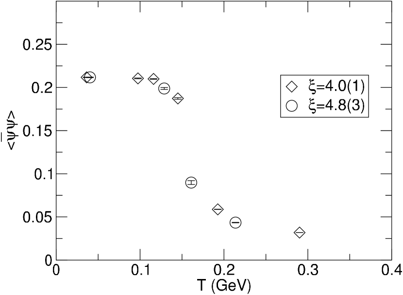
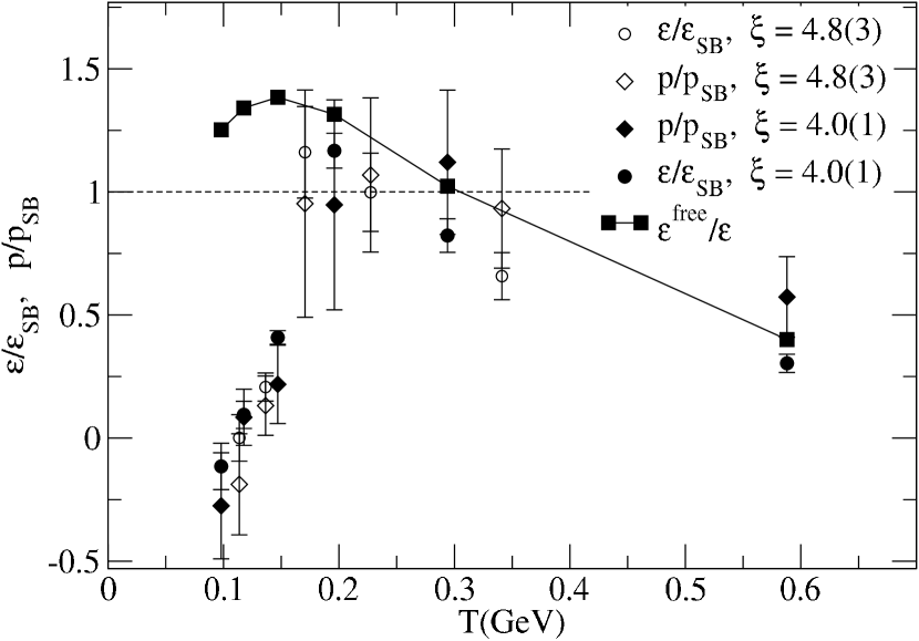
Figure 1: The temperature dependence of $\langle\overline{\psi}\psi\rangle$ in the region of $T_{c}$.

Figure 2: Energy and pressure in units of the Stefan-Boltzmann limit and a comparison with the free lattice theory (squares).

References

[1] QCD-TARO Collaboration: Ph. de Forcrand et al., Phys.Rev.D63:054501 (2001)
[2] F. Karsch, Nucl.Phys.B205[FS5], 285 (1982)
[3] S. Gottlieb et al., Phys.Rev.D35, 2531 (1987)
[4]MILC Collaboration: C. W. Bernard et al., Phys.Rev.D55, 6861 (1997)