Lanczos Methods for UV-Suppressed Fermions

Abstract

In this talk I indroduce lattice fermions with suppressed cutoff modes. Then I present Lanczos based methods for stochastic evaluation of the fermion determinant.

1 INTRODUCTION

There has been recent interest in the so-called ‘Ultraviolet slowing down’ of fermionic simulations in lattice QCD [1, 2, 3, 4, 5]. These studies try to address algortmically large fluctuations of the high end modes of the fermion determinant. The goal is to increase the signal-to-noise ratio of the infrared modes and to accelerate fermion simulations as well.

In fact, all the computational effort needed to treat UV-modes by above algorithms can be reduced to zero by suppressing them in the first place [6]. The lattice Dirac operator of this fermion theory is given by:

$$D=\frac{\mu}{a}\Gamma_{5}\tanh\frac{a\Gamma_{5}D_{W/S/O}}{\mu}$$ (1)

where $D_{W/s/o}$ is the input lattice Dirac operator, $a$ the lattice spacing and $\mu>0$ is a dimensionless parameter. For Wilson (W) and overlap (o) fermions as the input theory one has $\Gamma_{5}=\gamma_{5}$. For staggered fermions $\Gamma_{5}$ is a diagonal matrix with entries $+1/-1$ on even/odd lattice sites. The theory converges to the input theory in the contimuum limit and is local and unitary as shown in detail in [6]. The input theory is also recovered in the limit $\mu\rightarrow\infty$. For $\mu\rightarrow 0$ one has $D\rightarrow\mu$, i.e. a quenched theory.

Perturbative calculations with this theory are straightforward. In the following Wilson fermions are used as input. The inverse fermion propagator is given by:

$${\tilde{D}}(p)=\frac{\mu}{a}\gamma_{5}\tanh\frac{a{\tilde{H}_{W}}(p)}{\mu}$$ (2)

with $p=\{p_{\nu},\nu=1,\ldots,4\}$ being the four-momentum vector. As usual, gauge fields are parametrized by $su(3)$ elements, $U(x)_{\nu}=e^{iagA(x)_{\nu}}$ with $A(x)_{\nu}\in su(3)$ algebra, and the Wilson operator is written as a sum of the free and interaction terms: $D_{W}=D_{W}^{0}+D_{W}^{I}$. The splitting of the lattice Dirac operator is written in the same form:

$$D=D^{0}+D^{I},~{}~{}~{}~{}D^{0}=\frac{\mu}{a}\gamma_{5}\tanh\frac{aH_{W}^{0}}{\mu}$$

where the interaction term has to be determined. This can be done by expanding $D$ in terms of $a/\mu$:

$$D=D_{W}[\text{1\kern-2.41109ptl}+c_{1}(\frac{aH_{W}}{\mu})^{2}+c_{2}(\frac{aH_{W}}{\mu})^{4}+\cdots]$$ (3)

where $c_{1},c_{2},\ldots$ are real expansion coefficients. Calculation of $D^{I}$ is an easy task if one stays with a finite number of terms in the right hand side of (3). Also, the number of terms can be minimized using a Chebyshev approximation for the hyperbolic tangent.

2 COMPUTATIONAL METHODS

The effective action of the theory defined above can be written as:

$$S_{\text{eff}}=\text{tr}f(A)$$ (4)

where $A\in\mathbb{C}^{N\times N}$ and $f(s)$ is a real and smooth function of $s\in\mathbb{R}^{+}$. The matrix $A$ is assumed to be Hermitian and positive definite. Since the trace is dificult to obtain one can use the stochastic method of [7]. The method is based on evaluations of many bilinear forms of the type:

$${\mathcal{F}}(b,A)=b^{T}f(A)b$$ (5)

where $b\in\mathbb{R}^{N}$ is a random vector. The trace is estimated as an average over many bilinear forms. A confidence interval can be computed as described in detail in [7]. Here I will describe an alternative derivation of the Lanczos algorithm [8], which is used in [7] and in [9] as well. The full details of this study can be found at [10]. It uses familiar tools (in lattice simulations) such as sparse matrix invertions and Padé approximats.

The Padé approximation of a smooth and bounded function $f(.)$ in an interval can be expressed as a partial fraction expansion:

$$f(s)\approx\sum_{k=1}^{m}\frac{c_{k}}{s+d_{k}}$$ (6)

with $c_{k}\in\mathbb{R},d_{k}\geq 0,k=1,\ldots,m$. It is assumed that the right hand side converges to the left hand side when the number of partial fractions becomes large enough. For the bilinear form I obtain:

$${\mathcal{F}}(b,A)\approx\sum_{k=1}^{m}b^{T}\frac{c_{k}}{A+d_{k}\text{1\kern-2.41109ptl}}b$$ (7)

A first algorithm may be derived at this point. Having computed the partial fraction coefficients one can use a multi-shift iterative solver of [11] to evaluate the right hand side (7). The problem with this method is that one needs to store a large number of vectors that is proportional to $m$. This could be prohibitive if $m$ is say larger than $10$. However, it is easy to save memory if only the bilinear form (5) is needed (see [10] for details).

If a Padé approximation is not sufficient or difficult to obtain, the Lanczos method is the only alternative to evaluate exactly the bilinear forms of type (5). To see how this is realized I assume that the linear system $Ax=b$ is solved to the desired accuracy using the Lanczos algorithm. The algorithm produces the coefficients of the Lanczos matrix $T_{n}$, which is symmetric and tridiagonal. Its eigenvalues, the so called Ritz values, tend to approximate the extreme eigenvalues of the original matrix $A$. In the application considered here one can show that [10]:

$$\sum_{k=1}^{m}b^{T}\frac{c_{k}}{A+d_{k}\text{1\kern-2.41109ptl}}b=||b||^{2}\sum_{k=1}^{m}e_{1}^{T}\frac{c_{k}}{T_{n}+d_{k}{\text{1\kern-2.41109ptl}}_{n}}e_{1}$$ (8)

where ${\text{1\kern-2.41109ptl}}_{n}\in\mathbb{R}^{n\times n}$ is the identity matrix and $e_{1}$ is its first column. From this result and the convergence of the partial fractions to the matrix function $f(.)$, it is clear that:

$${\mathcal{F}}(b,A)\approx{\mathcal{\hat{F}}}_{n}(b,A)=||b||^{2}e_{1}^{T}f(T_{n})e_{1}$$ (9)

Note that the evaluation of the right hand side is a much easier task than the evaluation of the right hand side of (5). A straightforward method is the spectral decomposition of the symmetric and tridiagonal matrix $T_{n}=Z_{n}\Omega_{n}Z_{n}^{T}$, where $\Omega_{n}\in\mathbb{R}^{n\times n}$ is a diagonal matrix of eigenvalues $\omega_{1},\ldots,\omega_{n}$ of $T_{n}$ and $Z_{n}\in\mathbb{R}^{n\times n}$ is the corrsponding matrix of eigenvectors, i.e. $Z_{n}=[z_{1},\ldots,z_{n}]$. From (9) and the spectral form $T_{n}=Z_{n}\Omega_{n}Z_{n}^{T}$ it is easy to show that:

$${\mathcal{\hat{F}}}_{n}(b,A)=||b||^{2}e_{1}^{T}Z_{n}f(\Omega_{n})Z_{n}^{T}e_{1}$$ (10)

where the function $f(.)$ is now evaluated at individual eigenvalues of the tridiagonal matrix $T_{n}$. The eigenvalues and eigenvectors of a symmetric and tridiagonal matrix can be computed by the QL method with implicit shifts [12]. The method has an $O(n^{3})$ complexity. Fortunately, one can compute (10) with only an $O(n^{2})$ complexity. Closer inspection of eq. (10) shows that besides the eigenvalues, only the first elements of the eigenvectors are needed:

$${\mathcal{\hat{F}}}_{n}(b,A)=||b||^{2}\sum_{i=1}^{n}z_{1i}^{2}f(\omega_{i})$$ (11)

It is easy to see that the QL method delivers the eigenvalues and first elements of the eigenvectors with $O(n^{2})$ complexity. A similar formula (11) is suggested by [7] based on quadrature rules and Lanczos polynomials.

Algorithm 1 Lanczos algorithm to compute (5).

  Set $\beta_{0}=0,~{}\rho_{1}=1/||b||_{2},~{}q_{0}=o,~{}q_{1}=\rho_{1}b$

  for $~{}i=1,\ldots$ do

     $v=Aq_{i}$

     $\alpha_{i}=q_{i}^{{\dagger}}v$

     $v:=v-q_{i}\alpha_{i}-q_{i-1}\beta_{i-1}$

     $\beta_{i}=||v||_{2}$

     $q_{i+1}=v/\beta_{i}$

     $\rho_{i+1}=-(\rho_{i}\alpha_{i}+\rho_{i-1}\beta_{i-1})/\beta_{i}$

     if $1/|\rho_{i+1}|<\epsilon$ then

        $n=i$

        stop

     end if

  end for

  Set $~{}(T_{n})_{i,i}=\alpha_{i},~{}(T_{n})_{i+1,i}=(T_{n})_{i,i+1}=\beta_{i}$, otherwise $~{}(T_{n})_{i,j}=0$

  Compute $\omega_{i}$ and $z_{1i}$ by the QL method

  Evaluate (5) using (11)

Clearly, the Lanczos algorithm, Algorithm 1 has $O(nN)+O(n^{2})$ complexity, but it delivers an exact evaluation of (5) and for typical applications in lattice QCD the $O(n/N)$ overhead is small. The method of [7] computes the relative differences of (11) between two successive Lanczos steps and stops if they don’t decrease below a given accuracy. In order to perform the test their algorithm needs to compute the eigenvalues of $T_{i}$ at each Lanczos step $i$. This is illustrated in Fig. 1 where the convergence of the bilinear form (5) and extreme eigenvalues of $A$ are plotted.

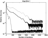
Figure 1: Relative differences of (11) (solid line), the largest (dashed line) and the smallest eigenvalue (dotted line) of $T_{n}$ for $f(s)=log(tanh\sqrt{s}),s>0$, $A=H_{W}^{2}$, and $b\in\mathbb{Z}_{2}$ noise on a $12^{3}\times 24$ lattice at $\beta=5.9$ and bare Wilson quark mass $m=-0.869$.

The figure sugests that one can compute the bilinear form less frequently than proposed by [7].

Acknowledgements. I would like to thank Philippe de Forcrand, Alan Irving and Tony Kennedy for discussions related to this talk.

References

- [1] A. C. Irving, J. C. Sexton, E. Cahill, J. Garden, B. Joo, S. M. Pickles, Z. Sroczynsk , Phys. Rev. D58 (1998) 114504
- [2] A. Duncan, E. Eichten, H. Thacker, Phys. Rev. D59 (1999) 014505
- [3] Ph. de Forcrand, Nucl. Phys. Proc. Suppl. 73 (1999) 822-824
- [4] M. Peardon, Nucl. Phys. B (Proc.Suppl.) 106&107 (2002) 3-11. See also M. Peardon, these proceedings.
- [5] A. Hasenfratz and F. Knechtli, Nucl. Phys. Proc. Suppl. 106 (2002) 1058-1060. See also A. Hasenfratz, these proceedings.
- [6] A. Boriçi, Lattice QCD with Suppressed High Momentum Modes of the Dirac Operator, hep-lat/0205011.
- [7] Z. Bai, M. Fahey, and G. H. Golub, J. Comp. Appl. Math., 74:71-89, 1996.
- [8] C. Lanczos, J. Res. Nat. Bur. Stand., 49 (1952), pp. 33-53
- [9] E. Cahill, A. Irving, C. Johnson, J. Sexton, Nucl. Phys. Proc. Suppl. 83 (2000) 825-827
- [10] A. Boriçi, Computational Methods for UV-Suppressed Fermions, hep-lat/0208034.
- [11] R. W. Freund, in L. Reichel and A. Ruttan and R. S. Varga (edts), Numerical Linear Algebra, W. de Gruyter, 1993
- [12] W.H. Press, S.A. Teukolsky, W.T. Vetterling, B.P. Flannery, Numerical Recipes in FORTRAN, Cambridge University Press, 1993