Static quark potential and string tension for compact U(1) in (2+1) dimensions.

Abstract

Compact U(1) lattice gauge theory in (2+1) dimensions is studied on anisotropic lattices using Standard Path Integral Monte Carlo techniques. We extract the static quark potential and the string tension from $1.0\leq\Delta\tau\leq 0.333$ simulations at $1.0\leq\beta\leq 3.0$. Estimating the actual value of the renormalization constant, (c = 44), we observe the evidence of scaling in the string tension for $1.4142\leq\beta\leq 2.5$; with the asymptotic behaviour in the large-$\beta$ limit given by $K\sqrt{\beta}=\mbox{e}^{(-2.494\beta+2.29)}$. Extrapolations are made to the extreme anisotropic or “Hamiltonian” limit, and comparisons are made with previous estimates obtained by various other methods in the Hamiltonian formulation.

I Introduction

Classical Monte Carlo simulations[1] of the path integral in Euclidean lattice gauge theory[2] have been very successful, and this is currently the preferred method for ab initio calculations in quantum chromodynamics (QCD) in the low energy regime. Monte Carlo approaches to the Hamiltonian version of QCD propounded by Kogut and Susskind[3] have been less successful, however, and lag at least ten years behind the Euclidean calculations. Our aim in this paper is to see whether useful results can be obtained for the Hamiltonian version by using the standard Euclidean Monte Carlo methods for anisotropic lattices[4], and extrapolating to the Hamiltonian limit in which the time variable becomes continuous, i.e. the lattice spacing in the time direction goes to zero. The Hamiltonian version of lattice gauge theory is less popular than the Euclidean version, but is still worthy of study. It can provide a valuable check of the universality of the Euclidean results[5], and it allows the application of many techniques imported from quantum many-body theory and condensed matter physics, such as strong coupling expansions[45], the t-expansion[7], the coupled-cluster method[8] and more recently the density matrix renormalization group[9] (DMRG). None of these techniques has proved as useful as Monte Carlo in (3+1) dimensions; but in lower dimensions they are more competitive.

A number of Quantum Monte Carlo methods have been applied to Hamiltonian lattice gauge theory in the past, with somewhat mixed results. A “Projector Monte Carlo” approach[10, 11] using a strong coupling representation for the gauge fields and a Greens Function Monte Carlo (GFMC) approach [13, 14], which makes use of a weak coupling representation of the gauge fields. However both the approaches run into difficulties in that the former approach runs into difficulties for non-Abelian models, and the later requires the use of a “trial wave function” to guide random walkers in the ensemble towards the preferred regions of configuration space[15]. This introduces a variational element into the procedure, in that the results may exhibit a systematic dependence on the trial wave function [16, 17, 18, 19, 20]. For this reason, we are forced to look yet again for an alternative approach.

As mentioned above our aim in this paper is to use standard Euclidean path integral Monte Carlo (PIMC) techniques for anisotropic lattices, and see whether useful results can be obtained in the Hamiltonian limit. Morningstar and Peardon[4] showed some time ago that the use of anisotropic lattices can be advantageous in any case, particularly for the measurement of glueball masses. We use a number of their techniques in what follows.

As a first trial of this approach, we treat the U(1) gauge model in (2+1)D, which is one of the simplest models with dynamical gauge degrees of freedom, and has also been studied extensively by other means (see Section II). Path integral Monte Carlo (PIMC) methods were applied to this model a long time ago by Hey and collaborators[21, 22], but the techniques used at that time were not very sophisticated, and the results were rather qualitative. Very little has been done since then using this approach on this particular model.

The rest of this paper is organised as follows. In section II we discuss the U(1) model in (2+1) dimensions in its lattice formulation, and outline some of the work done on it previously. The details of the simulations, including the generation of the gauge-field configurations, the construction of the Wilson loop operators, and the extraction of the potential and string tension estimates are described in section III. In section IV we present our main results for the mean plaquette, static quark potential, string tension. The static quark potential has not previously been exhibited for this model, as far as we are aware. Finally we make an extrapolation to the Hamiltonian limit, and comparisons are made with estimates obtained by other means in that limit. (Sec. 1V). We find that indeed the PIMC method can give better results than other methods, even in the Hamiltonian limit. Our conclusions are summarized in Sec. VI.

II THE U(1) MODEL

Consider the isotropic Abelian U(1) lattice gauge theory in three dimensions. The theory is defined by the action[2]

$$S=\beta\sum_{r,\mu,\nu}\mbox{ReTr}P_{\mu\nu}$$ (1)

where

$$\mbox{P}_{\mu\nu}(r)=\left[1-ReTr\{\mbox{U}_{\mu}(r)\mbox{U}_{\nu}(r+\hat{\mu})\mbox{U}_{\mu}^{\dagger}(r+\hat{\nu})\mbox{U}_{\nu}^{\dagger}(r)\right\}]$$ (2)

is the plaquette variable given by the product of the link variables taken around an elementary plaquette. The link variable $\mbox{U}_{\mu}(r)$ is defined by

$$\mbox{U}_{\mu}(r)=\mbox{exp}[ieaA_{\mu}(r)]=\mbox{exp}[i\theta_{\mu}(r)]$$ (3)

where in the compact form of the model, $\theta_{\mu}(r)(=eaA_{\mu}(r))\in[0,2\pi]$ represents the gauge field on the directed link $r\rightarrow r+\hat{\mu}$. The parameter $\beta$ is related to the bare gauge coupling by

$$\beta=\frac{1}{g^{2}}$$ (4)

where $g^{2}=ae^{2}$, in (2+1) dimensions.

The lattice U(1) model in (2+1) dimensions has been studied by many authors, and possesses some important similarities with QCD (for a more extensive review, see for example ref. [12]). If one takes the “naive” continuum limit at a fixed energy scale, one regains the simple continuum theory of non-interacting photons[25]; but if one renormalizes or rescales in the standard way so as to maintain the mass gap constant, then one obtains a confining theory of free massive bosons. Polyakov[26] showed that a linear potential appears between static charges due to instantons in the lattice theory; and Göpfert and Mack[27] proved that in the continuum limit the theory converses to a scalar free field theory of massive bosons. They found that in that limit the mass gap behaves as

$$am_{D}=\sqrt{\frac{8\pi^{2}}{g^{2}}}\mbox{exp}\bigg{(}-\frac{\pi^{2}}{g^{2}}v(0)\bigg{)}$$ (5)

while the string tension is bounded by

$$a^{2}\sigma=c\sqrt{\frac{g^{2}}{2\pi^{2}}}\mbox{exp}(-\frac{\pi^{2}}{g^{2}}v(0))$$ (6)

where $v(0)$ is the Coulomb potential at zero distance, and has a value in lattice units

$$v(0)=0.2527$$ (7)

for the isotropic case. They argue that eq. (6) represents the true asymptotic behaviour of the string tension, where the constant $c$ is equal to $8$ in classical approximation. The theory has a non-vanishing string tension for arbitrary large $\beta$, similiar to behaviour expected for the string tension in non-abelian lattice gauge theories in 4-dimensions.

In the small-$\beta$ limit the string tension behaves as:

$$a^{2}\sigma=-\mbox{ln}\beta/2+....$$ (8)

and the large-$\beta$ behaviour is given by eq. (6).

Similar behaviour will apply in the anisotropic case. Generalizing discussions by Banks et al[45] and Ben-Menahem[46], we find (see the appendix A) that the exponential factor takes exactly the same form in the anisotropic case, with a Coulomb potential $v(0)$ changing to $0.3214$ in the Hamiltonian limit.

For an anisotropic lattice, the gauge action becomes[47, 48]

$$S=\beta_{s}\sum_{r,i<j}P_{ij}(r)+\sum_{r,i}\beta_{t}P_{it}(r)$$ (9)

where $P_{ij}$ and $P_{it}$ are the spatial and temporal plaquette variables respectively. In the classical limit

$$\beta_{s} = \frac{a_{t}}{e^{2}a_{s}^{2}}=\frac{1}{g^{2}}\Delta\tau$$ (10)

$$\beta_{t} = \frac{1}{e^{2}a_{t}}=\frac{1}{g^{2}}\frac{1}{\Delta\tau}$$ (11)

where $\Delta\tau=a_{t}/a_{s}$ is the anisotropy parameter, $a_{s}$ is the lattice spacing in the space direction, and $a_{t}$ is the temporal spacing. The above action can be written as

$$S = \beta\bigg{[}\Delta\tau\sum_{r}\sum_{i<j}\bigg{(}1-\cos\theta_{ij}(r)\bigg{)}+\frac{1}{\Delta\tau}\sum_{r,i}\bigg{(}1-\cos\theta_{it}(r)\bigg{)}\bigg{]}$$ (12)

In the limit $\Delta\tau\rightarrow 0$, the time variable becomes continuous, and we obtain the Hamiltonian limit of the model (modulo a Wick rotation back to Minkowski space). The Hamiltonian version of the model has been studied by many methods: some recent studies include series expansions [28, 5], finite-lattice techniques[30], the t-expansion [31, 32], and coupled-cluster techniques[33, 34], as well as Quantum Monte Carlo methods[23, 36, 37, 12]. Quite accurate estimates have been obtained for the string tension and the mass gaps, which can be used as comparison for our present results. The finite-size scaling properties of the model can be predicted using an effective Lagrangian approach combined with a weak-coupling expansion [38], and the predictions agree very well with finite-lattice data [12].

Some analytic results for the model in the weak-coupling approximation appear in the appendix.

III METHODS

A Path Integral Monte Carlo algorithm

We perform standard path integral Monte Carlo simulations on a finite lattice of size $N_{s}^{2}\times N_{\tau}$, where $N_{s}$ is the number of lattice sites in the space direction and $N_{\tau}$ in the temporal direction, with spacing ratio $\Delta\tau=a_{t}/a_{s}$. By varying $\Delta\tau$ it is possible to change $a_{t}$, while keeping the spacing in the spatial direction fixed. The simulations were performed on lattices with $N_{s}=16$ sites in each of the two spatial directions and $N_{t}=16-64$ in the temporal direction for a range of couplings $\beta=1-3$.

The ensembles of field configurations were generated by using a Metropolis algorithm. Starting from an arbitrary initial configuration of link angles, we successively update link angles $\theta_{\mu}(\vec{r},\tau)$ at positions $(\vec{r},\tau)$ which are chosen randomly each time. We propose a change $\Delta\theta$ to this link angle, which is randomly drawn from a uniform distribution on $[-\Delta,\Delta]$, where $\Delta$ is adjusted for each set of parameters to give an acceptable “hit rate” around 70-80%. The change is accepted or rejected according to the standard Metropolis procedure.

For high anisotropy ($\Delta\tau<<1$), any change in a time-like plaquette will produce a large change in the action, whereas changes to the space-like plaquettes will cause a much smaller change in the action. This makes the system very “stiff” against variations in the time-like plaquettes, and therefore very slow to equilibrate, with long autocorrelation times. To alleviate this problem, we used a Fourier update procedure[39, 40]. Here proposed changes are made to space-like links which are designed to alter space-like plaquette values much more than the time-like plaquette values. At randomly chosen intervals and random locations, we propose a non-local change $\Delta\theta(\vec{r},\tau)=X\sin k(\tau-\tau_{0})$ on a “ladder” of space-like links extending half a wavelength $(\lambda=2\pi/k)$ in the time direction, where both $k$ and $X$ are randomly chosen at each update from uniform distributions in $[0,\pi/2]$. We replaced approximately $30\%$ of the ordinary Metropolis updates with Fourier updates for anisotropy $\Delta\tau>0.444$ and $50\%$ for highly anisotropic cases ($\Delta\tau<0.444$). These moves satisfy the requirements of detailed balance and ergodicity for the algorithm.

A single sweep involves attempting $N$ changes to randomly chosen links of the lattice, where $N(=3N_{t}N_{s}^{2})$ is the total number of links on the lattice. The first several thousand sweeps are discarded to allow the system to relax to equilibrium. Fig. 1 shows measurements of the mean plaquette for $\beta=2.0$ and $\Delta\tau=1.0$, and it can be seen that equilibrium is reached after about 50,000 thousand sweeps, with the measurements fluctuating about the equilibrum value thereafter. For highly anisotropic cases the system was much slower to equilibrate, despite the Fourier acceleration, and in the worst case the equilibration time was of order 100,000 thousand sweeps.

After discarding the initial sweeps, the configurations were stored every 250 sweeps thereafter for later analysis. Ensembles of about 1,000 configurations were stored to measure the static quark potential and glueball masses at each $\beta$ for $\Delta\tau\geq 0.4$, and 1,400 configurations for $\Delta\tau\leq 0.333$. Measurements made on these stored configurations were grouped into 5 blocks, and then the mean and standard deviation of the final quantities were estimated by averaging over the “block averages”, treated as independent measurements. Each block average thus comprised 50,000 - 70,000 sweeps.

B Interquark Potential

The static quark-antiquark potential, $V(\bf{r})$ for various spatial separations $\bf{r}$ is extracted from the expectation values of the Wilson loops. The timelike Wilson loops are expected to behave as:

$$W({\bf r},\tau)\simeq Z({\bf r})\mbox{exp}\big{[}-\tau V({\bf r})]+{\hbox{(excited state contributions)}}$$ (13)

We have averaged only over loops $({\bf x_{0}},\tau_{0})\rightarrow({\bf x_{0}+r},\tau_{0})\rightarrow({\bf x_{0}+r},\tau_{0}+\tau)\rightarrow({\bf x_{0}},\tau_{0}+\tau)\rightarrow({\bf x_{0}},\tau_{0})$ which follow either two sides of a rectangle between ${\bf x_{0}}$ and ${\bf x_{0}+r}$ or a single-step ‘staircase’ route, to estimate $W({\bf r},\tau)$. To suppress the excited state contributions, a simple APE smearing technique[41, 42] was used on the space-like variables. In this technique an iterative smearing procedure is used to construct Wilson loop (and glueball) operators with a very high degree of overlap with the lowest-lying state. In our single-link smoothing procedure, we replace every space-like link variable by

$$U_{i}\rightarrow P\left[\alpha U_{i}+\frac{(1-\alpha)}{2}\sum_{s}U_{s}\right]$$ (14)

where the sum over “s” refers to the “staples”, or 3-link paths bracketing the given link on either side in the spatial plane, and P denotes a projection onto the group U(1), achieved by renormalizing the magnitude to unity. We used a smearing parameter $\alpha=0.7$ and up to 10 iterations of the smearing process.

To further reduce the statistical errors, the timelike Wilson loops were constructed from “ thermally averaged” temporal links[43]. That is, the temporal links $U_{t}$ in each Wilson loop were replaced by their thermal averages

$$\bar{U_{t}}=\int dUU\exp(-S[U])/\int dU\exp(-S[U])$$ (15)

where the integration is done over the one link only, and depends on the neighbouring links. For the U(1) model, the result can easily be computed in terms of Bessel functions involving the “staples” adjacent to the link in question. This was done for all temporal links except those adjacent to the spatial legs of the loop, which are not “independent”[43]. The procedure has a dramatic effect in reducing the statistical noise, by up to an order of magnitude 10, which corresponds to a factor 100 in the statistics[4].

Fig. 2 shows an example of the exponential decrease of the $4\times 1$Wilson loop $W(\vec{r},\tau)$ with $\tau$. Estimates of the potential can now be found from the ratios of successive loop values:

$$V({\bf r})=\frac{1}{\Delta\tau}\mbox{ln}\bigg{[}\frac{W({\bf r},\tau+\Delta\tau)}{W({\bf r},\tau)}\bigg{]}$$ (16)

This ratio is expected to be independent of $\tau$ for $\tau>>0$. Fig.3 shows the effective potential as a function of Euclidean time, $\tau$, obtained from $\Delta\tau=1.0$ at $\beta=2.0$ for $r=4$ simulation. We find that ratio reaches its plateau behavior at very early Euclidean times, which reflects a good optimized smearing. We used $\tau=1$ to make our estimates of $V(\bf{r})$.

IV Simulation results at finite temperature

Simulations were carried out for lattices of $N_{s}^{2}\times N_{t}$ sites, with $N_{s}=16$ and $N_{t}$ ranging from 16 to 48 sites, with periodic boundary conditions. Each run involved 250,000 sweeps (350,000 for high anisotropy) of the lattice, with 60,000 sweeps (100,000 high anisotropy) discarded to allow for equilibrum, and configurations recorded every 250 sweeps thereafter. Coupling values from $\beta=1.0$ to 3.0 were explored at anisotropies $\Delta\tau$ ranging from 1 to 1/3. We fixed $\Delta\tau=16/N_{t}$ in the first pass, so that the lattice size $T=N_{t}a_{t}$ in the time direction remains constant, corresponding to a fixed (low) temperature.

A Mean Plaquette

The mean plaquette, or equivalently the $1\times 1$ Wilson loop, was measured for various $16\times 16\times N_{t}$ (with $N_{t}$ = 16 up to 48) sizes and for a variety of $\beta$ values, ranging from strong coupling to weak coupling regime. Fig. 4 shows the behaviour of the mean spatial plaquette $<P>$ for different $\beta$, at fixed $\Delta\tau=1$ (isotropic case). At small coupling (large $\beta$) the plaquette expectation value is expected to approach 1, and conversely it approaches 0 in the high coupling (small $\beta$) limit. The plot also shows the $O(\beta^{4})$ strong-coupling [51] and $O(1/\beta^{5})$ weak coupling [50] expansion. The dashed curve represents the weak-coupling series and strong-coupling series is represented by the solid curve. As can be seen that the data follow closely the weak coupling expansion down to $\beta=2.0$ and strong coupling expansion upto $\beta=1.70$ and the results agree very well. The variation of $<P>$ with coupling is extremely smooth, with no sign of phase transition, as we should expect. The cross-over from strong to weak coupling seems, from the Monte Carlo data, to take place quite raidly in the region $\beta\approx 1.8-2.0$. Horsley and Wolff [50] investigates the effect of finite size lattice in their weak-coupling expansion calculations. They find that such effects enter at order $1/\beta^{2}$ as a correction of order $1/l^{D}$, where $l$ is the lattice size and $D$ is the number of dimensions. Thus for U(1) in (2+1) and $l>10$, finite size effects should be essentially negligible.
Fig. 5 shows a plot of our estimates of $<P>$ as a function of anisotropy ${\Delta\tau}^{2}$ for the case $\beta=\sqrt{2}$. We would like to make contact with previous Hamiltonian studies by showing that the mean plaquette value approaches to previously known values in the Hamiltonian limit $\Delta\tau\rightarrow 0$. The extrapolation was performed using a simple cubic fit in powers of $\Delta\tau^{2}$. In this limit our results agree very well with the Hamiltonian estimate obtained by Hamer et al[17]. The estimates of the mean plaquette $<P>$ in the Hamiltonian limit are graphed as a function of $\beta$ in Fig.6 and compared with the series estimates at strong and weak coupling [28], and Greens function Monte Carlo results[17]. At large $\beta$, the data is in good agreement with predictions of weak-coupling perturbation theory. At small $\beta$, the data follow closely the strong-coupling and Greens function Monte Carlo estimates, except at very small $\beta$. We attribute the discrepnacy to the finite-temperature effects and a better agreement is expected at zero-temperature [52].

B Static quark potential and string tension

The effective potential is obtained from the ratio of successive Wilson loop values:

$$V_{\tau}({\bf{r}})=\mbox{ln}\bigg{(}\frac{W({\bf{r}},\tau+\Delta\tau)}{W({\bf{r}},\tau)}\bigg{)}$$ (17)

Fig. 7 shows a graph of the static quark potential V(R) as a function of radius R at $\beta=2.0$ and $\Delta\tau=1.0$. To extract the string tension, the curve is well fitted by a form

$$V(R)=a+b\ln R+\sigma R,$$ (18)

including a logarithmic Coulomb term as expected for classical QED in (2+1) dimensions which dominates the behaviour at small distances, and a linear term as predicted by Polyakov[26] and Göpfert and Mack[27] dominating the behaviour at large distances. The linear behaviour at large distances is very clear, but the data do not extend to very small distances, so there is no real test of the presumed logarithmic behaviour in this regime.

Figs. 8 shows the behaviour of the fitted value of the string tension $K(=a^{2}\sigma)$ as a function of $\beta$ for the isotropic case ( $\Delta\tau=1$), plotted in comparison to results predicted for string tension using the large-$\beta$ approximation (eq. 6). We also include the strong-coupling values and show the leading order strong-coupling prediction (eq. 7). As can be seen that our estimates of the string tension, in the weak-coupling region are much larger than the Villain prediction, though slopes are more or less well determined. However one does not expect agreement of precise magnitude, since our estimates are obtained using Wilson action, and not the Villian approximation. But one does expect that the slope of the string tension in both cases should ultimately be the same as one approaches the continuum limit. Mack and Göpfert [27] argued that eq. (6) represents the true asymptotic behaviour of the string tension, apart from the value of the renormalization constant $c$. Such a behaviour was obtained by a semi-classical treatment of the theory with the effective action without the correction terms. Thus it is possible that eq. (6), including the normalization constant, becomes exact as $1/\beta\rightarrow 0$, if one estimates the actual value of $c$. We estimated the actual value of $c$ by graphing the $\mbox{e}^{2.494\beta}\times 4.443K$ against $1/\beta$ and extrapolating to $1/\beta\rightarrow 0$. Using estimated value of the renormalization constant, $c=44$, we plotted the asymptotic form of the string tension in weak-coupling limit in comparison to our estimates. The result agrees very well with our estimates.

Fig. 9 shows the behaviour of the string tension ($K$) as a function of the anisotropy ${\Delta\tau}^{2}$, for fixed coupling $\beta=\sqrt{2}$. An extrapolation to the Hamiltonian limit $\Delta\tau\rightarrow 0$ is performed by a simple cubic fit. Again the extrapolation agrees rather well with earlier Hamiltonian estimates[12]. Note that this quantity depends rather strongly on $\Delta\tau$: there is a factor of three difference between the values at $\Delta\tau=0$ and $\Delta\tau=1$. Extrapolating to $\Delta\tau\rightarrow 0$, estimates of the string tension in the Hamiltonian limit, for various $\beta$ values are obtained. The plot of these estimates, in comparison to the large-$\beta$ prediction of eq. (6) is shown in Fig. 10. As can be seen, the weak-coupling results, with estimated value for constant coefficient, agree very well with our estimates. The comparison with the theoretical prediction using Villian form is not bad either, especially in the large-$\beta$ region. In this region, upto $\beta\approx 1.8$, the results agree well within errors and slopes are very well defined.

Fig. 11 shows the plot of Hamiltonian estimates as a function of $\beta$, plotted in comparison to the previous estimates obtained from strong-coupling [8], Greens function Monte Carlo [17] and finite-size scaling [38] The agreement with the series expansion and GFMC results is once again excellent. The estimates of finite-size scaling describe the data at $\beta=2.0$.

V Summary and conclusion

In this paper, we used numerical simulation techniques on anisotropic lattices for U(1) model in (2+1) dimensions to obtain a clear picture of the confinement and improve our knowledge of the string tension. Our first aim was to implement Path Integral Monte Carlo method to the U(1) model, which is one of the simplest models and has been studied by various other methods. It seems to work extremely well for the mean plaquette in the strong-coupling and weak-coupling regimes. The simulation results were extrapolated to $\Delta\tau\rightarrow 0$, and Hamiltonian estimates for mean plaquette were obtained. A comparison was made with the previous estimates obtained in this limit and agreement was excellant. The second aim was the get a better picture of the confinement and the numerical study of the asymptotic behaviour of the string tension in the large-$\beta$ limit. It was shown that at large separations the U(1) theory in (2+1) dimensions shows a linear behaviour as predicted by Polyakov. However, the presumed logarithmic term could not be tested as our data do not extend to very small separations. The estimates of string tension have confirmed very well the weak-coupling predictions, provided that one takes the estimated value of the constant coefficient $c$ rather than its value in the classical approximation using effective action without correction terms. For $\beta<2.0$, the data is in good agreement with $O(\beta^{2})$ strong-coupling predictions. Once again our Hamiltonian estimates for the string tension fit very well with the series and GFMC results.

This seems to suggest that PIMC does work better than other methods, as stated by Ceperley. The first clear picture of the static quark potential has been obtained, showing clear evidence of the linear confining potential at large distance predicted by Polyakov. Our results from the PIMC do appear to be in agreement with results of the series expansions.

A Weak-coupling prediction using Villian approximation

Here we extend the discussion of the weak-coupling behaviour of the mass gap to the anisotropic case, following the discussions of Banks, Myerson and Kogut[45] and Ben-Menahem[46]. This can be probed by means of the expectation value of the Wilson loop, $<W(C)>$, which for pure gauge theory is given by

$$<W(C)>=\frac{Z(J)}{Z(0)}$$ (A1)

where

$$Z(J)=\prod_{r,\mu}\bigg{\{}\int d\theta_{\mu}(r)\bigg{\}}\mbox{exp}\left[-S-i\sum_{r,\mu}J_{\mu}(r)\theta_{\mu}(r)\right]$$ (A2)

and $J_{\mu}(r)$ is a vector field associated with a rectangular contour C of width R and length T. The extra piece of action associated with the external charge is

$$S_{J}=\int d^{3}rJ_{\mu}(r)\theta_{\mu}(r)$$

For a point charge, $S_{J}$ is given by the path integral of the gauge field along the world line of the charge. Therefore we choose

$$J_{\mu}(r)=\left\{\begin{array}[]{ll}1&\textrm{if $r\rightarrow r+\hat{\mu}$ is on C}\\ -1&\textrm{if $r+\hat{\mu}\rightarrow$ is on C}\\ 0&\textrm{otherwise}\end{array}\right.$$ (A3)

and this current is conserved: $\Delta_{\mu}J_{\mu}(r)=0$. We will assume a spacelike Wilson loop for this discussion.

It is convenient to work in the temporal gauge

$$\theta_{t}(\vec{r})=0$$ (A4)

Then one can separate the angular variable $\theta_{i}(r)$ into longitudinal and transverse parts,

$$\theta_{i}(r)=\triangle_{i}\rho(r)-\epsilon_{ij}\frac{1}{\triangle_{1}^{2}+\triangle_{2}^{2}}\triangle_{j}\theta(r)$$ (A5)

whence it follows that $\theta_{ij}(r)=\theta(r)$. In the temporal gauge eq. (A2) can be written as

$$Z(J)=\prod_{r}\int_{-\infty}^{\infty}\{d\theta(r)\}\mbox{exp}\left[-\beta\Delta\tau\sum_{r}\bigg{(}1-\cos\theta(r)\bigg{)}-\frac{\beta}{2\Delta\tau}\sum_{r}\theta(r)\frac{\bar{\triangle}_{t}\triangle_{t}}{\bar{\triangle}_{i}\triangle_{i}}\theta(r)+i\sum_{r}J_{i}\epsilon_{ij}\frac{1}{\triangle_{k}^{2}}\triangle_{j}\theta(r)\right]$$ (A6)

with $\triangle_{i}^{2}=\triangle_{1}^{2}+\triangle_{2}^{2}$. $\bar{\triangle}$ and ${\triangle}$ are defined are the lattice difference operators. To calculate the path integral we replace the potential term by its Villain form

$$\mbox{e}^{-\beta(1-\cos\theta(r))}\rightarrow\sum_{l=-\infty}^{\infty}\mbox{e}^{il\theta}\mbox{e}^{-\beta}I_{l}(\beta).$$ (A7)

where $I_{\l}(\beta)$ is the modified Bessel function and $\mbox{exp}(il\theta)$ is the character of the plaquette variable in the $l$th irreducible representation of the compact U(1) group.

For large $\beta$ the modified Bessel function can be approximated by

$${e}^{-\beta}I_{l}(\beta)\approx\frac{1}{\sqrt{2\pi\beta}}\mbox{e}^{-l^{2}/2\beta}$$ (A8)

The Gaussian integration over $\theta(r)$ reduces the path integral to

$$Z(J) \propto \prod_{r}\sum_{l(r)=-\infty}^{\infty}\mbox{exp}\left[-\frac{1}{2\beta\Delta\tau}\sum_{r}l(r)\bigg{(}\Delta\tau^{2}\frac{\bar{\triangle}_{i}\triangle_{i}}{\bar{\triangle}_{t}\triangle_{t}}+1\bigg{)}l(r)-\frac{\Delta\tau}{\beta}\sum_{r}l(r)\frac{1}{\bar{\triangle}_{t}\triangle_{t}}\epsilon_{ij}J_{i}\triangle_{j}\right.$$ (A10)

$$\left.-\frac{\Delta\tau}{2\beta}\sum_{r}J_{i}(r)\frac{1}{\bar{\triangle}_{t}\triangle_{t}}J_{i}(r)\right]$$

The convergence of the sum over $l$ can be improved by making use of the Poisson summation formula,

$$\sum_{l=-\infty}^{\infty}h(l)=\sum_{m=-\infty}^{\infty}\int d\phi h(\phi)\mbox{e}^{2i\pi mr}$$ (A11)

where $h$ is an arbitrary function.

Substituting $l(r)=\triangle_{t}L(r)$ and using eq. (A8), Eq. (A10) becomes

$$Z(J) \propto \prod_{r}\int_{-\infty}^{\infty}d\phi(r)\sum_{m(r)=-\infty}^{\infty}\left[\mbox{exp}\bigg{\{}-\frac{1}{2\beta\Delta\tau}\sum_{r}\phi(r)\bigg{(}\Delta\tau^{2}\bar{\triangle}_{i}\triangle_{i}+\bar{\triangle}_{t}\triangle_{t}\bigg{)}\phi(r)\right.$$ (A14)

$$\left.+\frac{\Delta\tau}{\beta}\sum_{r}\phi(r)\frac{1}{\triangle_{t}}\epsilon_{ij}J_{i}\triangle_{j}+2i\pi\sum_{r}m(r)\phi(r)\bigg{\}}\right]$$

$$\times\mbox{exp}\left[-\frac{\Delta\tau}{2\beta}\sum_{r}J_{i}(r)\frac{1}{\bar{\triangle}_{t}\triangle_{t}}J_{i}(r)\right]$$

Finally doing the Gaussian integral over $\phi$ yields;

$$Z(J) \propto \prod_{r}\sum_{m(r)=-\infty}^{\infty}\mbox{exp}\left[-2\pi^{2}\beta\Delta\tau\sum_{r}m(r)\bigg{(}\frac{1}{\Delta\tau^{2}\bar{\triangle}_{i}\triangle_{i}+\bar{\triangle}_{t}\triangle_{t}}\bigg{)}m(r)\right.$$ (A17)

$$\left.+2\pi i\Delta\tau^{2}\sum_{r}m(r)\bigg{(}\frac{1}{\Delta\tau^{2}\bar{\triangle}_{i}\triangle_{i}+\bar{\triangle}_{t}\triangle_{t}}\bigg{)}\frac{1}{\triangle_{t}}\epsilon_{ij}J_{i}\triangle_{j}\right]$$

$$\times\mbox{exp}\left[-\frac{\Delta\tau}{2\beta}\sum_{r,i}J_{i}\frac{1}{\Delta\tau^{2}\bar{\triangle}_{i}\triangle_{i}+\bar{\triangle}_{t}\triangle_{t}}J_{i}(r)\right]$$

The partition function, $Z(J=0)$, is given by

$$Z(J=0)=\prod_{r}\sum_{m(r)=-\infty}^{\infty}\mbox{exp}\left[-2\pi^{2}\beta\sum_{r,r^{\prime}}m(r)G(r-r^{\prime})m(r^{\prime})\right]$$ (A18)

where

$$G(r-r^{\prime})=\frac{\Delta\tau\delta_{rr^{\prime}}}{\Delta\tau^{2}\bar{\triangle}_{i}\triangle_{i}+\bar{\triangle}_{t}\triangle_{t}}$$ (A19)

is a three-dimensional lattice massless propagator.

The propagator can be expressed as a momentum integral:

$$G(r,t)=\int_{-\pi}^{\pi}\frac{dk_{0}}{2\pi}\int_{-\pi}^{\pi}\frac{dk_{1}}{2\pi}\int_{-\pi}^{\pi}\frac{dk_{2}}{2\pi}\frac{\Delta\tau\mbox{e}^{ik.r+k_{0}t)}}{4\sin^{2}k_{0}/2+\Delta\tau^{2}\bigg{(}4-2\cos k_{1}-2\cos k_{2}\bigg{)}}$$ (A20)

For the isotropic lattice ($\Delta\tau=1$), $G(k=0)=0.2527$; while in the limit $\Delta\tau\rightarrow\infty$, $G(k=0)$ takes the value $0.3214$.
The resulting partition function may be written as

$$Z(J)=Z_{spin-wave}Z_{ext}Z_{monopoles}$$ (A21)

where

$$Z_{spin-wave} = \int[d\chi]\mbox{exp}\left[-\frac{1}{\beta}\sum_{r,i}\bigg{(}\triangle_{i}\chi(r)\bigg{)}^{2}\right]$$ (A22)

$$Z_{ext} = \mbox{exp}\left[-\frac{1}{2\beta}\sum_{r,r^{\prime},i}J_{i}(r)G(r-r^{\prime})J_{i}(r^{\prime})\right]$$ (A23)

$$Z_{monopole} = \sum_{r}\sum_{m(r)=-\infty}^{\infty}\mbox{exp}\left[-2\pi^{2}\beta\sum_{r,r^{\prime}}m(r)G(r-r^{\prime})m(r^{\prime})+2i\pi\sum_{r,r^{\prime}}G(r-r^{\prime})\eta(r)m(r)\right]$$ (A24)

The first factor in eq. (A20), the “spin-wave” piece, contributes the ordinary Coulomb part to the potential between the external charges. The rest of the eq. (A20) is the partition sum of the Coulomb gas of magnetic monopoles interacting with a stationary current loo via $G(r-r^{{}^{\prime}})$. This three-dimensional Coulomb gas is always in a plasma phase. The only thing that changes with $\beta$ is the density of the monopoles which decays exponentially to zero as $\beta$ increases. The monopole density generated by the external loop and coupling to the lattice monopoles m(r) is a dipole sheet along the surface spanning the contour C. Thus eq. (A20) represents a dipole sheet immersed in a monopole gas, which interacts directly with the dipole sheet. The gas becomes polarized, and the monopoles of opposite polarity accumulate on the two sides of the sheet, screening both the magnetic field away from the sheet and the monopole-monopole interaction, thus minimizing the energy of the system. This gives the correlation function a finite range, whose inverse is interpreted as a mass of the scalar field.
In the naive continuum limit, the Coulomb self-energy of the monopoles blows up and their density goes to zero exponentially. This causes the coefficient of the linear force law to go to zero and one regains the usual continuum theory, i.e., free electromagnetism in three dimensions; but if one renormalizes or rescales in the standard way so as to maintain the mass gap constant, then one obtains a confining theory of free massive bosons. The detailed analysis of Polyakov[26] shows that the sheet cannot be screened completely and there is a finite energy left that binds the quarks through a potential which grows linearly with separation. Polyakov showed that for arbitrarily large finite $\beta$, theory has a mass gap and there appears a linear potential appears between static charges due to instantons in the lattice theory.
Splitting the exponent in eq. (A20) into pieces with $r=r^{\prime}$ and $r\neq r^{\prime}$, the monopole partition sum can be written as

$$Z_{monopole}(J) = \prod_{r}\int d\phi(r)\mbox{exp}\left[-\frac{1}{8\pi^{2}\beta}\sum_{r}\bigg{(}\Delta_{i}\phi(r)\bigg{)}^{2}-\sum_{m=-\infty}^{\infty}2\pi^{2}\beta G_{0}\right.$$ (A26)

$$\left.-2i\pi\sum_{r}\eta(r)m(r)+i\sum_{r}\phi(r)m(r)\right]$$

For large $\beta$, one can neglect all the monopoles with charge other than 0, $\pm 1$ in the sum, since the monopoles with a higher charge gets extra powers of $\mbox{e}^{-\beta}$. Applying the large-$\beta$ approximation to the monopole partition function, the above equation can be written, in the naive continuum limit, as

$$Z_{monopole}(J)\approx\int D\phi\mbox{exp}\left[-\frac{g^{2}}{4\pi^{2}}\int\bigg{\{}\frac{1}{2}(\partial_{i}\phi)^{2}-M^{2}\cos\bigg{(}\phi+2\pi\eta\bigg{)}\bigg{\}}d^{3}x\right]$$ (A27)

where the lattice photon mass $M$ is given by

$$M^{2}=\frac{8\pi^{2}}{g^{2}a^{3}}\mbox{e}^{-2\pi^{2}G_{0}/g^{2}a}.$$ (A28)

At this point out analysis parallels the work of original work of Banks et al [45].
The the expectation value of the Wilson loop becomes

$$<W(C)> \approx \mbox{exp}\left[-\frac{1}{2\beta}\sum_{r,r^{\prime},i}J_{i}(r)G(r-r^{\prime})J_{i}(r^{\prime})\right]\prod_{r}\int d\phi(r)\mbox{exp}\left[-\frac{1}{8\pi^{2}\beta}\sum_{r}\bigg{(}\Delta_{i}\phi(r)\bigg{)}^{2}\right.$$ (A30)

$$\left.-2\mbox{e}^{-2\pi^{2}\beta G_{0}}\sum_{r}\bigg{(}1-\cos(\phi(r)+2\pi\eta(r))\bigg{)}\right]$$

B Large-$\beta$ prediction in Hamiltonian formulation

We now do the Hamiltonian study of U(1) model in (2+1) dimensions using weak coupling perturbation theory. The Hamiltonian formulation of compact U(1) gauge theory has been studied by Banks et al. [45] and Drell et al. [24] following the Kogut and Susskind approach [3].
Consider the anisotropic Wilson gauge action for U(1) model in (2+1) dimensions,

$$S=\beta\left[\frac{1}{\Delta\tau}\sum_{i}P_{it}+\Delta\tau\sum_{i<j}P_{ij}\right]$$ (B1)

where we made assumed the lattice symmetric in spatial directions with $a_{s}=1$ and $a_{t}=\Delta\tau$.
The plaquette variable is given by

$$P_{ij}=1-\cos\theta_{ij}^{P}$$

and $\beta=1/g^{2}$.

In the weak coupling approximation

$$\cos\theta_{ij}^{P}\simeq 1-\frac{1}{2}{\theta_{ij}^{P}}^{2}$$ (B2)

The plaquette angles $\theta^{P}$ are related to the link angles $A_{l}$ by

$$\theta^{P}(\tilde{n}^{{}^{\prime}},\tilde{\hat{k}})=\epsilon_{ijk}\left[A_{l}(\b{n},\hat{i})-A_{l}(\tilde{n}+\hat{j},\hat{i})+A_{l}(\tilde{n}+\hat{i},\hat{j})A_{l}(\tilde{n},\hat{j})\right]$$ (B3)

where $(\tilde{n}^{{}^{\prime}},\tilde{\hat{k}})$ denote a plaquette centered at $\tilde{n}^{{}^{\prime}}$ and oriented in the $\hat{k}$ while $(\tilde{n}^{{}^{\prime}},\hat{i})$ describes a link that starts at site $\tilde{n}$ in the direction $\hat{i}$, with

$$\tilde{n}^{{}^{\prime}}=\tilde{n}+(\frac{\hat{i}+\hat{j}}{2})$$

The Fourier transformations of the plaquette angles and the link angle give

$$\theta_{\tilde{k}}(\hat{\mu}) = \frac{1}{\sqrt{N}}\sum_{\tilde{n}^{{}^{\prime}}}\mbox{e}^{-i\tilde{k}\cdot\tilde{n}^{{}^{\prime}}}\theta_{P}(\tilde{n}^{{}^{\prime}},\hat{\mu})$$ (B4)

$$A_{\tilde{k}}q(\hat{\mu}) = \frac{1}{\sqrt{N}}\sum_{\tilde{n}}\mbox{e}^{-i\tilde{k}.\tilde{n}}A_{l}(\tilde{n},\hat{\mu})$$ (B5)

where $N=N_{s}^{2}N_{t}$ is the total number of sites; then

$$A_{\tilde{k}}^{\dagger}(\hat{\mu}) = A_{-\tilde{k}}(\hat{\mu})$$ (B6)

$$\theta_{\tilde{k}}^{\dagger}(\hat{\mu}) = \theta_{-\tilde{k}}(\hat{\mu})$$ (B7)

Therefore eq. (B3) can be written as

$$\theta_{\tilde{k}}(\hat{\mu})=\sum_{\hat{\nu}}G_{\tilde{k}}(\hat{\mu},\hat{\nu})A_{\tilde{k}}(\hat{\nu})$$ (B8)

where

$$G_{\b{k}}(\hat{\mu},\hat{\nu})=2i\sum_{\nu,\rho}\epsilon_{\mu\nu\sigma}\mbox{e}^{-ik_{\nu}/2}\sin(k_{\sigma}/2)$$ (B9)

Choosing the temporal gauge $A_{0}=0$, the time-like plaquette contributions, in the weak coupling approximation, become:

$$\sum_{\tilde{n}}\theta_{i0}^{2}(\tilde{n}) = \sum_{\tilde{k}}\theta_{i0,\tilde{k}}^{\dagger}\theta_{i0,\tilde{k}}$$ (B10)

$$= \sum_{\tilde{k}}A_{\tilde{k}}^{\dagger}(\hat{i})A_{\tilde{k}}(\hat{i})\times 4\sin^{2}(k_{0}/2)$$ (B11)

while the space-like plaquette contribution becomes:

$$\sum_{\tilde{n}}\theta_{12}^{2}(\tilde{n}) = \sum_{\tilde{k}}\theta_{12,\tilde{k}}^{\dagger}\theta_{12,\tilde{k}}$$ (B12)

$$= \sum_{\tilde{k}}A_{\tilde{k}}^{\dagger}R_{\tilde{k}}A_{\tilde{k}}$$ (B13)

where $A_{\tilde{k}}$ and $R_{\tilde{k}}$ are the vectors and matrices, $(2\times 2)$ in $(\hat{1},\hat{2})$ square, respectively, and $R_{\tilde{k}}=G_{\tilde{k}}^{\dagger}G_{\tilde{k}}$. Therefore

$$R_{\tilde{k}}=\left(\begin{array}[]{ccc}\sin^{2}(k_{y}/2)&-\mbox{e}^{i(k_{x}/2-k_{y}/2)}\sin k_{x}/2\sin k_{y}/2\\ -\mbox{e}^{i(k_{y}/2-k_{x}/2)}\sin k_{x}/2\sin k_{y}/2&\sin^{2}(k_{x}/2)\end{array}\right)$$ (B14)

The matrix $R_{\tilde{k}}$ is hermitian, and has eigenvalues:

$$\lambda_{\tilde{k}}(1) = 4\sum_{i=1}^{2}\sin^{2}(k_{i}/2)$$ (B15)

$$\lambda_{\tilde{k}}(1) = 0$$ (B16)

We can define a unitary transformation

$$\omega_{\tilde{k}}=u_{\tilde{k}}A_{\tilde{k}}$$ (B17)

which diagonalizes the matrix $R_{\tilde{k}}$:

$$u_{\tilde{k}}=\frac{i}{sqrt{\sin^{2}k_{x}/2+\sin^{2}k_{y}/2}}\left(\begin{array}[]{ccc}-\mbox{e}^{ik_{x}/2}\sin(k_{y}/2)&\mbox{e}^{ik_{y}/2)}\sin k_{x}/2\\ -\mbox{e}^{ik_{x}/2)}\sin k_{x}/2&\mbox{e}^{ik_{y}/2}\sin^{2}(k_{x}/2)\end{array}\right)$$ (B18)

The components of $\omega_{\tilde{k}}$ are

$$\omega_{\tilde{k}}(1) = \frac{i}{c_{1}}\left[\mbox{e}^{-ik_{y}/2)}\sin k_{x}/2A_{\b{k}}(\hat{2})-\mbox{e}^{ik_{x}/2}\sin(k_{y}/2)A_{\b{k}}(\hat{2})\right]$$ (B19)

$$\omega_{\tilde{k}}(2) = \frac{i}{c_{1}}\left[\mbox{e}^{-ik_{x}/2)}\sin k_{x}/2A_{\b{k}}(\hat{1})+\mbox{e}^{ik_{y}/2}\sin(k_{y}/2)A_{\b{k}}(\hat{2})\right]$$ (B20)

where $c_{1}=\sqrt{\sin^{2}k_{x}/2+\sin^{2}k_{y}/2}$.
The component of $w_{\tilde{k}}$ corresponding to the zero eigenvalue is

$$\tilde{\omega}_{\tilde{k}}=\frac{i}{c_{1}}\left[(1-\mbox{e}^{-ik_{x}})A_{\tilde{k}}(\hat{x})+(1-\mbox{e}^{-ik_{y}})A_{\tilde{k}}(\hat{y})\right].$$ (B21)

This vanishes at all orders and is an ”ignorable” coordinate.
Thus the action eq. (B1) can be written as

$$S = \frac{\beta}{2}\sum_{\tilde{k}}\left[\Delta\tau\bigg{(}\triangle_{\tilde{k}}\omega_{\tilde{k}}^{\dagger}(1)\omega_{\tilde{k}}(1)\right]$$ (B23)

$$+\frac{1}{\Delta\tau}\left[4\sin^{2}(k_{0}/2)\sum_{\mu=1}^{2}\omega_{\tilde{k}}^{\dagger}(\hat{\mu})\omega_{\tilde{k}}(\hat{\mu})\right]+\mbox{const}.$$

where

$$\triangle_{\tilde{k}}=4\left[\sin^{2}k_{1}/2+\sin^{2}k_{2}/2\right]$$ (B24)

Therefore the partition function can be written as

$$Z=\prod_{\tilde{k}}\{\int d\omega{\tilde{k}}\}\mbox{e}^{-S[\omega]}$$ (B25)

where the action can be written in the following form:

$$s[\omega] \approx \frac{\beta}{2}\sum_{\tilde{k}}\left[\omega_{\tilde{k}}^{\dagger}(1)\omega_{\tilde{k}}(1)\bigg{(}\Delta\tau\triangle_{\tilde{k}}+\frac{4}{\Delta\tau}\sin^{2}(k_{0}/2)\bigg{)}\right.$$ (B27)

$$\left.+\omega_{\tilde{k}}^{\dagger}(2)\omega_{\tilde{k}}(2)\bigg{(}\frac{4}{\Delta\tau}\sin^{2}(k_{0}/2)\bigg{)}\right]$$

Now $\omega_{\tilde{k}}$ is the ignorable coordinate and will be ignored from here on.
The partition function becomes

$$Z \approx \prod_{\b{k}}\left[\frac{2\pi}{\beta}\frac{1}{\bigg{(}\Delta\tau\triangle_{\b{k}}+\frac{4}{\Delta\tau}\sin^{2}(k_{0}/2)\bigg{)}}\right]^{1/2}$$ (B28)

$$= \mbox{exp}\left[\frac{N}{2}\mbox{ln}(\frac{2\pi}{\beta})-\frac{1}{2}\sum_{\b{k}}\mbox{ln}\bigg{(}(\Delta\tau\triangle_{\b{k}}+\frac{4}{\Delta\tau}\sin^{2}(k_{0}/2)\bigg{)}\right]$$ (B29)

This lead to the following free energy density:

$$f=\frac{1}{2N}\sum_{\tilde{k}}\mbox{ln}\left[\frac{\beta}{2\pi}d(\tilde{k})\right]$$ (B30)

where

$$d(\tilde{k})=(\Delta\tau\triangle_{\tilde{k}}+\frac{4}{\Delta\tau}\sin^{2}(k_{0}/2)$$ (B31)

1 Mean space-like plaquette

At weak coupling the cosine term in the space-like part may be expanded in the powers of $\theta_{P}$. Therefore

$$<\cos\theta_{ij}> = 1-\frac{1}{2}<\theta_{ij}^{2}>$$ (B32)

$$= 1-\frac{1}{2}<\frac{1}{N}\sum_{\tilde{k}}\triangle_{\tilde{k}}\omega_{\tilde{k}}^{\dagger}(1)\omega_{\tilde{k}}(1)>$$ (B33)

where

$$<\omega_{\tilde{k}}^{\dagger}(1)\omega_{\tilde{k}}(1)> = \frac{\int d\omega_{\tilde{k}}\mbox{e}^{-\frac{\beta}{2}d(\tilde{k})\omega_{\tilde{k}}^{\dagger}\omega_{\tilde{k}}}\omega_{\tilde{k}}^{\dagger}\omega_{\tilde{k}}}{\int d\omega_{\tilde{k}}\mbox{e}^{-\frac{\beta}{2}d(\tilde{k})\omega_{\tilde{k}}^{\dagger}\omega_{\tilde{k}}}}$$ (B34)

Using the integrals

$$\int_{-\infty}^{\infty}d\omega\mbox{e}^{-a\omega^{2}} = \sqrt{\frac{\pi}{2}}$$ (B35)

$$\int_{-\infty}^{\infty}d\omega\omega^{2}\mbox{e}^{-a\omega^{2}} = \frac{1}{2a}\sqrt{\frac{\pi}{2}}$$ (B36)

we get

$$<\omega_{\tilde{k}}^{\dagger}\omega_{\tilde{k}}>=\frac{1}{\beta d(\tilde{k}}$$ (B37)

Therefore

$$<\cos\theta_{ij}>=1-\frac{1}{2\beta N}\sum_{\tilde{k}}\frac{\triangle_{\tilde{k}}}{d(\tilde{k})}$$ (B38)

Now consider the “cylindrical limit”, $N_{t}\rightarrow\infty$, $\triangle\tau\rightarrow 0$: In this limit the sum term in the right hand side of the above equation becomes;

$$\sum_{\b{k}}\frac{\triangle_{\tilde{k}}}{d(\tilde{k})} \rightarrow \sum_{\vec{k}}\triangle(\vec{k})\frac{N_{t}}{2\pi}\int_{0}^{2\pi}dk_{0}\frac{1}{\triangle\tau+\frac{4}{\triangle\tau}\sin^{2}(k_{0}/2)}$$ (B39)

$$= \sum_{\vec{k}}\frac{N_{t}}{2\pi}2\int_{0}^{2\pi}\frac{dx}{\bigg{(}\triangle\tau\triangle(\vec{k})+\frac{x^{2}}{\triangle\tau}\bigg{)}}$$ (B40)

$$= \sum_{\vec{k}}\frac{N_{t}}{\pi}\frac{\pi}{2\sqrt{\triangle(\vec{k})}}$$ (B41)

In the bulk limit, $N\rightarrow\infty$, this becomes;

$$\approx \frac{N_{t}{2}.(\frac{N_{s}}{2\pi})^{2}}{\int}\int_{0}^{2\pi}dk_{x}dk_{y}\sqrt{4\bigg{(}\sin^{2}k_{x}/2+\sin^{2}k_{y}/2}$$ (B42)

$$= \frac{N_{t}}{2}.2N_{s}^{2}C_{1}^{(2)}$$ (B43)

where

$$C_{1}^{(2)} = \frac{1}{N_{s}^{2}}\sum_{\vec{k}}(1-\gamma_{\vec{k}})^{1/2}$$ (B44)

$$= \frac{1}{2N_{s}^{2}}\sum_{\vec{k}}\Delta^{1/2}(\vec{k})$$ (B45)

$$= 0.958$$ (B46)

is a standard lattice sum.
Therefore

$$<\cos\theta_{ij}> = 1-\frac{1}{2\beta}C_{1}^{(2)}$$ (B47)

$$= 1-\frac{g^{2}}{2}C_{1}^{(2)}$$ (B48)

$$= 1-0.479g^{2}$$ (B49)

This result agrees with the estimates in the Hamiltonian limit [5] Now taking the bulk limit in isotropic case, we get

$$\sum_{\tilde{k}}\frac{\Delta(\vec{k})}{d(\tilde{k})}\rightarrow\frac{N}{(2\pi)^{3}}\int\int_{0}^{2\pi}\int dk_{x}dk_{y}dk_{0}\frac{(\sin^{2}k_{x}/2+\sin^{2}k_{y}/2)}{(\sin^{2}k_{x}/2+\sin^{2}k_{y}/2+\sin^{2}k_{0}/2)}$$ (B50)

By symmetry, we can easily find that

$$\sum_{\tilde{k}}\frac{\Delta(\vec{k})}{d(\tilde{k})}=\frac{2N}{3}$$ (B51)

Therefore

$$<\cos\theta_{ij}>=1-\frac{g^{2}}{3}$$ (B52)

2 Mean time-like plaquette

In weak coupling approximation the time-like plaquette can be written as

$$\frac{1}{2}\sum_{i=1}^{2}<\cos\theta_{i0}> = 1-\frac{1}{4}\sum_{i=1}^{2}<\theta_{i0}^{2}>$$ (B53)

$$= 1-\frac{1}{4}<\frac{1}{N}\sum_{\tilde{k}}4\sin^{2}k_{0}/2A_{\tilde{k}}^{\dagger}(\hat{i})A_{\tilde{k}}(\hat{i})>$$ (B54)

$$= 1-\frac{1}{4N}<\sum_{\tilde{k}}4\sin^{2}k_{0}/2\bigg{(}\omega_{\tilde{k}}^{\dagger}(\hat{1})\omega_{\tilde{k}}(\hat{1})+\omega_{\tilde{k}}^{\dagger}(\hat{2})\omega_{\tilde{k}}(\hat{2}\bigg{)}>$$ (B55)

Now

$$<\omega_{\tilde{k}}^{\dagger}(\hat{1})\omega_{\tilde{k}}(\hat{1})+\omega_{\tilde{k}}^{\dagger}(\hat{2})\omega_{\tilde{k}}(\hat{2}\bigg{)}>=\frac{1}{\beta d(\tilde{k})}+\frac{\Delta\tau}{4\beta\sin^{2}k_{0}/2}$$ (B56)

$$\frac{1}{2}\sum_{i=1}^{2}<\cos\theta_{i0}>=1-\frac{g^{2}}{4N}\sum_{\tilde{k}}4\sin^{2}k_{0}/2\left[\frac{1}{d(\tilde{k})}+\frac{\Delta\tau}{4\sin^{2}k_{0}/2}\right]$$ (B57)

The term in the square brackets can be written as

$$\sum_{\tilde{k}}4\sin^{2}k_{0}/2\left[\frac{1}{d(\tilde{k})}+\frac{\Delta\tau}{4\sin^{2}k_{0}/2}\right] = \frac{N}{(2\pi)^{3}}\int\int_{0}^{2\pi}\int dk_{x}dk_{y}dk_{0}\Delta\sin^{2}k_{0}\left[\frac{1}{\sin^{2}k_{0}/2}\right.$$ (B59)

$$\left.+\frac{1}{\sin^{2}k_{0}/2+\sin^{2}k_{0}/2+{\Delta\tau}^{2}(\sin^{2}k_{x}/2+\sin^{2}k_{y}/2)}\right]$$

$$= \left\{\begin{array}[]{ll}0&(\Delta\tau=0)\\ N(1+1/3)&(\Delta\tau=1)\end{array}\right.$$ (B62)

Thus the mean time-like plaquette gives;

$$\frac{1}{2}\sum_{i=1}^{2}<\cos\theta_{i0}>=\left\{\begin{array}[]{ll}0&(\Delta\tau=0)\\ 1-\frac{g^{2}}{3}&(\Delta\tau=1)\end{array}\right.$$ (B63)

as is expected.

3 Expectation value of Wilson loop

The expectation value of the Wilson loop is given by

$$<W(R,T)>=\frac{1}{Z}\prod_{\tilde{k}}\int d\omega_{\tilde{k}}W_{c}\mbox{e}^{-S[\omega]}$$ (B64)

where the Wilson loop operator is given by

$$W_{C}=\frac{1}{2}\left[\prod_{l\in C}\mbox{e}^{A_{l}}+\mbox{h.c}\right]$$ (B65)

Taking the separation R in the $x$ direction, for simplicity, the Fourier transformation of above equation) is

$$W_{C}=\mbox{exp}\left[\frac{i}{\sqrt{N}}\sum_{\tilde{k}}\sum_{\tilde{x},\mu\in C}\mbox{e}^{i\tilde{k}.\tilde{x}}A_{\tilde{k}}(\hat{\mu}\right]+\mbox{h.c}$$ (B66)

We now consider the contribution from class of “zero modes” with $k=(k_{0},\vec{k}=0)$. These modes are likely to be responsible for the dominant finite-size corrections [5], i.e.,

$$W_{0}(R,t)=\mbox{exp}\left[\frac{i}{\sqrt{N}}\sum_{k_{0}}A_{k_{0},\vec{0}}(\hat{x})R\bigg{(}\mbox{e}^{ik_{0}x_{01}}-\mbox{e}^{ik_{0}x_{02}}\bigg{)}\right]$$ (B67)

Recalling that $A_{0}=0$, the above equation becomes

$$W_{0}(R,t) = \mbox{exp}\left[\frac{2}{\sqrt{N}}\sum_{k_{0}}A_{k_{0},\vec{0}}(\hat{x})R\mbox{e}^{ik_{0}(\frac{x_{01}+x_{02}}{2})}\sin k_{0}T/2\right]$$ (B68)

$$= \mbox{exp}\left[\frac{2}{\sqrt{N}}\sum_{k_{0}}\omega_{\tilde{k}}(\hat{1})R\sin k_{0}T/2\right]$$ (B69)

where $T=x_{02}-x_{01}$ and we have ignored the $\mbox{e}^{ik_{0}(\frac{x_{01}+x_{02}}{2})}$. Therefore

$$<W_{0}(R,T)>=\frac{1}{Z(0)}\prod_{k_{0}}\int d\omega_{k_{0}}(\hat{1})\mbox{exp}\left[\frac{2}{\sqrt{N}}\omega_{k_{0}}R\sin(k_{0}T/2)-\frac{\beta}{2\Delta\tau}4\sin^{2}(k_{0}/2)\omega_{k_{0}}^{\dagger}\omega_{k_{0}}\right]$$ (B70)

Let

$$\frac{\beta}{2\Delta\tau}4\sin^{2}(k_{0}/2)=c(k_{0});$$

then the numerator of above equation can be written as

$$I_{k_{0}}=\int_{-\infty}^{\infty}d\omega\mbox{exp}\left[-c(k_{0}\bigg{(}\omega-i\frac{R\sin(k_{0}T/2)}{\sqrt{N}c(k_{0})}\bigg{)}^{2}\right]\mbox{exp}\left[-\frac{R^{2}\sin^{2}(k_{0}T/2)}{\sqrt{N}c(k_{0})}\right]$$ (B71)

Therefore the expectation value of the Wilson loop is given by

$$<W_{0}(R,T)> = \prod_{k_{0}}\mbox{exp}\left[\frac{R^{2}\sin^{2}(k_{0}T/2)}{\sqrt{N}2\beta\sin^{2}(k_{0})}\right]$$ (B73)

$$\mbox{exp}\left[-\frac{R^{2}\Delta\tau}{2N_{s}^{2}N_{t}\beta}\frac{N_{t}}{2\pi}\int_{0}^{2\pi}dk_{0}\frac{\sin^{2}(k_{0}T/2}{\sin^{2}(k_{0}/2}\right]$$

Now consider the cylindrical limit, $N_{t}\rightarrow\infty$, $\Delta\tau\rightarrow 0$. In this limit

$$\frac{1}{2\pi}\int_{0}^{2\pi}dk_{0}\frac{\sin^{2}(k_{0}T/2)}{\sin^{2}(k_{0}/2)}\rightarrow T$$ (B74)

Therefore

$$<W_{0}(R,T)> = \mbox{exp}\left[-\frac{g^{2}}{2}(\frac{R}{N_{s}})^{2}T\Delta\tau\right]$$ (B76)

$$\mbox{exp}\bigg{(}-\sigma\times\mbox{area}\bigg{)}$$

Where

$$\sigma_{eff}=\frac{g^{2}}{2}(\frac{R}{N_{s}^{2}})=\frac{g^{2}}{2}(\frac{R}{L^{2}})$$ (B77)

For R=L, i.e., for pair of Polyakov loops mapping around the lattice in the spatial direction, we get

$$\sigma_{eff}=\frac{g^{2}}{2L}$$ (B78)

This corresponds to the value calculated by Hamer and Zheng [5], $\sigma=1/L$, for a string wrapping around the entire lattice, if we multiply by an extra factor $g^{2}/2$ coming from renormalizing Hamiltonian. As is obvious that for smaller loops, the effective string tension is less.

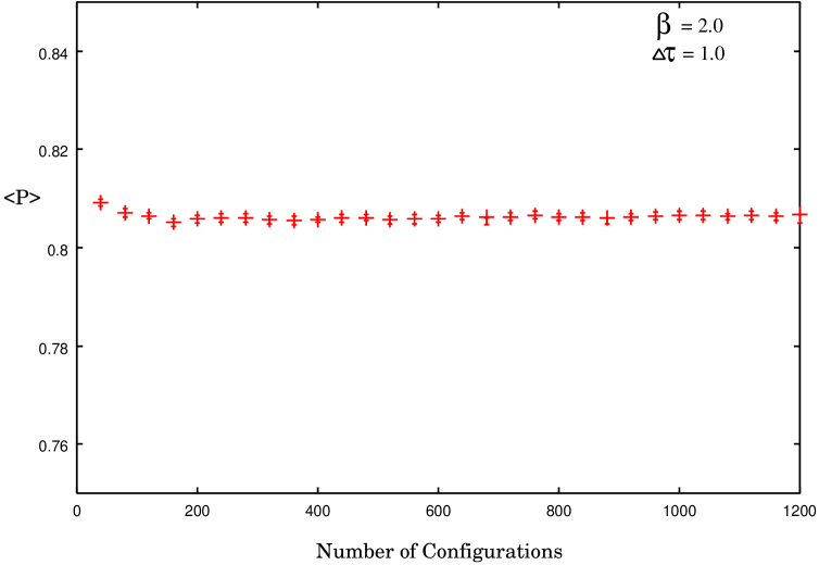
FIG. 1.: Plot of plaquette average against the number of configurations. The loop average is seen to reach its equilibrum value, after discarding the initial number of sweeps (50000 for $16^{3}$ lattice).

FIG. 2.: Plot of a $4\times 1$ Wilson loop against $\tau$ from $\Delta\tau=1.0$ simulations for $\beta=2.0$

FIG. 3.: Ratio of the Wilson loops as a function of $\tau$ for fixed $x$ and $y$ from $\beta=2.0$ and $\Delta\tau=1.0$ simulations. The ratio is seen reaching its plateau at very early times and is very close to its asymptotic large-$t$ plateau.

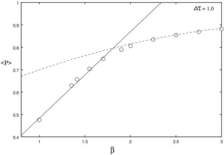
FIG. 4.: Plot of average plaquette as a function of $\beta$. The $\circ$ symbols label our Monte Carlo estimates. The solid curve represents the $O(\beta^{4})$ strong-coupling expansion [49] and the dashed curve represents the $O(1/\beta^{5})$ weak-coupling expansion [50].

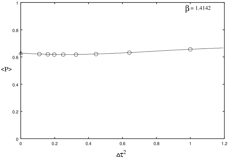
FIG. 5.: The mean plaquette as a function of $\Delta\tau^{2}$ at $\beta=1.4142$. The solid curve is cubic fit, in powers of $\Delta\tau^{2}$, to the data extrapolated to the Hamiltonian limit. $\triangle$ symbol represents the series estimates [27] in that limit.

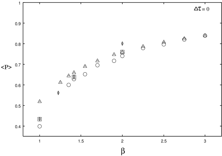
FIG. 6.: Mean plaquette estimates against $\beta$ at $\Delta\tau=0$. The earlier estimates from strong-coupling expansion and Greens function Monte Carlo are represented by $\Diamond$ and $\Box$ symbols respectively. Our Monte Carlo estimates and weak-coupling expansion results, (Eq.B31), are represented by $\bigcirc$ and $\triangle$ respectively.

FIG. 7.: The static-quark potential, $V(R)$ as a function of the separation R. This plot includes the measurements from $\beta=2.0$ for $\Delta\tau=1.0$ with 10 sweeps of smearing at smearing parameter $\alpha=0.7$. The analysis errors are smaller than the plot symbols. The dashed line is the fit to the form $V(R)=a+bR+c\mbox{log}(R)$.

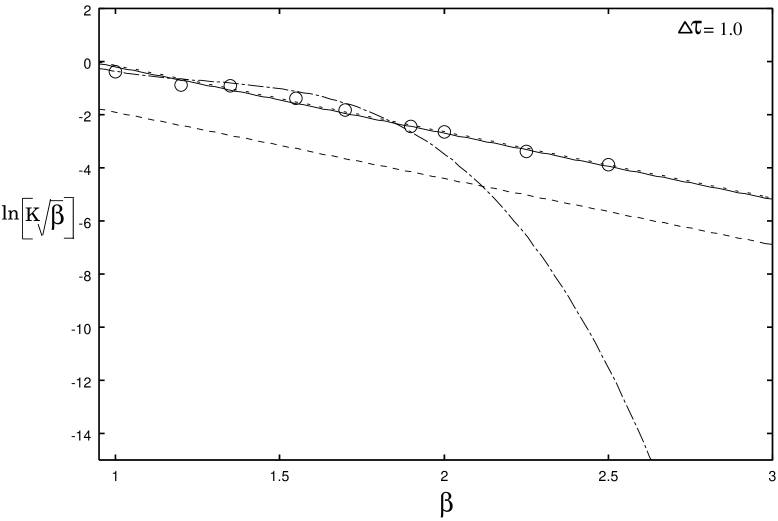
FIG. 8.: String tension as a function of $\beta$. The solid curve represents the weak-coupling result using Villian approximation, with our estimated value for renormalization constant, $c$(=44) and the dotted curve coinciding with the solid curve is the linear fit to our Monte Carlo estimates. The dashed curve represents the scaling behaviour predicted by Mack and Göpfert (eq.6) and the dash-dot curve is the strong coupling result of eq. (8).

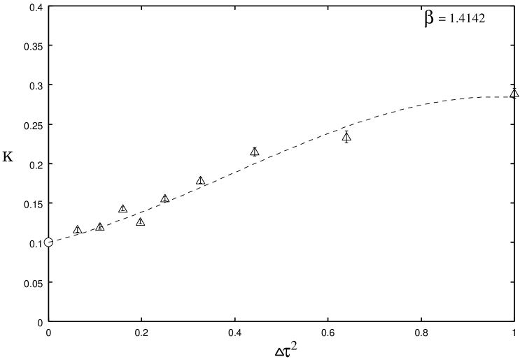
FIG. 9.: String tension against $\Delta\tau^{2}$ at $\beta=1.4142$. Extrapolation to Hamiltonian limit is performed by a cubic fit shown by the dashed line and the earlier Hamiltonian estimate [27] is shown by $\bigcirc$.

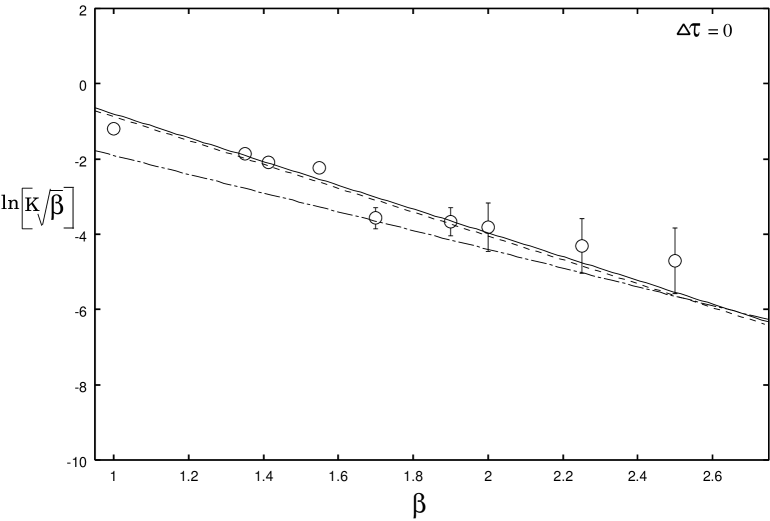
FIG. 10.: plot showing the estimates of string tension in the Hamiltonian limit as a function of $\beta$. The solid line is the weak-coupling prediction with estimated value of the renormalization constant $c$, and dashed line is the linear fit to our Monte Carlo data. The dash-dot curve represents the large-$\beta$ prediction of Mack and Gopfert using Villian approximation.

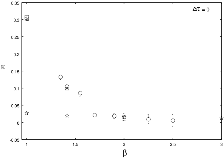
FIG. 11.: Hamiltonian estimates of string tension as a function of $\beta$. Our estimates of string tension are labeled by $\bigcirc$ symbol. Earlier results from series expansion [8], Greens function Monte Carlo [17], and finite size scaling [37] are labeled by $\triangle$, $\Box$ and $\star$ respectively. As is seen that our estimates make a very good contact with earlier Hamiltonian estimates obtained by many other techniques

REFERENCES

- [1] M. Creutz, Phys. Rev. Letts. 43, 553 (1979)
- [2] K.G. Wilson, Phys. Rev. D10, 2445 (1974)
- [3] J. Kogut and L. Susskind, Phys. Rev. D11, 395 (1975)
- [4] C.J. Morningstar and M. Peardon, Phys. Rev. D56, 4043 (1997)
- [5] C. J. Hamer, M. Sheppeard, W. H. Zheng and D. Schütte, Phys. Rev. D54, 2395 (1996)
- [6] T.Banks, S. Raby, L. Susskind, J. Kogut, D.R.T. Jones, P.N. Scharbach and D.K. Sinclair, Phys. Rev. D15, 1111 (1977)
- [7] D. Horn and M. Weinstein, Phys. Rev. D30, 1256 (1984)
- [8] Guo Shuohong, Zheng Weihong and Liu Jiunmin, Phys. Rev. D38, 2591 (1988)
- [9] T.M.R. Byrnes, P.Sriganesh, R.J. Bursill and C.J. Hamer, to be published in Phys. Rev. D
- [10] D.Blankenbecler and R.L. Sugar, Phys. Rev. D27, 1304( 1983)
- [11] T.A. DeGrand and J. Potvin, Phys. Rev. D31, 871 (1985)
- [12] C. J. Hamer, K. C. Wang and P. F. Price, Phys. Rev. D50, 4693 (1994)
- [13] S. A. Chin, J. W. Negele and S. E. Koonin, Ann. Phys. (N.Y.) 157, 140 (1984)
- [14] D. W. Heys and D. R. Stump, Phys. Rev. D28, 2067 (1983)
- [15] Kalos M. H., J. Comp. Phys. 1, 257 (1966); D. M. Ceperley and M. H. Kalos, in Monte Carlo Methods in Statistical Mechanics, ed. K. Binder (Springer-Verlag, New York, 1979).
- [16] M. Samaras and C. J. Hamer, Aust. J. Phys. 52, 637 (1999)
- [17] C.J. Hamer, R.J. Bursill and M. Samaras, Phys. Rev. D62, 054511 (2000)
- [18] C.J. Hamer, R.J. Bursill and M. Samaras, Phys. Rev. D62, 074506 (2000)
- [19] K.S. Liu, M.H. Kalos and G.V. Chester, Phys. Rev. A10 303 (1974)
- [20] P. A. Whitlock, D. M. Ceperley, G. V. Chester and M. H. Kalos, Phys. Rev. B19, 5598 (1979)
- [21] J. Ambjorn, A.J.G. Hey and S. Otto, Nucl. Phys. B210, 347 (1982)
- [22] P.D. Coddington, A.J.G. Hey, A.A. Middleton and J.S. Townsend, Phys. Letts. B175, 64 (1986)
- [23] S. A. Chin, C. Long and D. Robson, Phys. Rev. Letts. 57, 60 (1986),
- [24] S.D. Drell, H.R. Quinn, vetitsky and M. Weinstein, Phys. Rev. bf D19, 619 (1979)
- [25] L. Gross, Commun. Math. Phys. 92, 137 (1983)
- [26] A.M. Polyakov, Phys. Lett. 72B, 477 (1978)
- [27] M. Göpfert and G. Mack, Commun. Math. Phys. 82, 545 (1982)
- [28] C. J. Hamer, J. Oitmaa, and Zheng Weihong, Phys. Rev. D45, 4652 (1992)
- [29] C.J.Hamer, Zheng Weihong and J. Oitmaa, Phys. Rev. D53, 1429 (1996)
- [30] A.C. Irving, J.F. Owens and C.J. Hamer, Phys. Rev. D28, 2059 (1983)
- [31] D. Horn, G. Lana and D. Schreiber, Phys. Rev. D36, 3218 (1987)
- [32] C.J. Morningstar, Phys. Rev. D46, 824 (1992)
- [33] A. Dabringhaus, M.L. Ristig and J.W. Clark, Phys. Rev. D43, 1978 (1991)
- [34] X.Y. Fang, J.M. Liu and S.H. Guo, Phys. Rev. D53, 1523 (1996)
- [35] S.J. Baker, R,.F. Bishop and N.J. Davidson, Phys. Rev. D53, 2610 (1996).
- [36] S. E. Koonin, E. A. Umland and M. R. Zirnbauer, Phys. Rev. D33, 1795 (1986)
- [37] C. M. Yung, C. R. Allton and C. J. Hamer, Phys. Rev. D33, 1795 (1986)
- [38] C. J. Hamer and Zheng Weihong, Phys. Rev. D48, 4435 (1993)
- [39] G.G. Batrouni, G.R. Katz, A.S. Kronfeld, G.P. Lepage, B.Svetitsky and K.G. Wilson, Phys. Rev. D32, 2736 (1985)
- [40] C.T.H. Davies, G.G. Batrouni, G.R. Katz, A.S. Kronfeld, G.P. Lepage, P. Rossi, B. Svetitsky and K.G. Wilson, Phys. Rev. D41, 1953 (1990)
- [41] M. Albanese et al., Phys. Lett. B192, 163 (1987)
- [42] M. Teper, Phys. Lett. B183, 345 (1986); K.Ishikawa, A. Sato, G. Schierholz and M. Teper, Z. Phs. C21, 167 (1983).
- [43] G. Parisi, R. Petronzio and F. Rapuano, Phys. Lett. 128B, 418 (1983).
- [44] M.J. Teper, Phys. Rev. D59, 014512 (1999)
- [45] T. Banks, R. Myerson and J. Kogut, Nucl. Phys. B129, 493 (1977).
- [46] S. Ben-Menahem, Phys. Rev. D20, 1923 (1979).
- [47] F. Karsch, Nucl. Phys. B205, 285 (1982).
- [48] G. Burgers, Nucl. Phys. B304, 587 (1988).
- [49] F. Brandstacter et al., Nucl. Phys. B345, 709 (1990).
- [50] R. Horsley and U. Wolff, Phys. Letts. B105, 290 (1981).
- [51] G. Bhanot and M. Creutz, Phys. Rev. D21, 2892 (1980).
- [52] M. Loan, and C.J. Hamer, to be published