Gauge Problem of Monopole Dynamics in SU(2) Lattice Gauge Theory

Abstract:

Gauge problem of monopole dynamics is studied in $SU(2)$ lattice gauge theory. We study first abelian and monopole contributions to the static potential in four smooth gauges, i.e., Laplacian Abelian (LA), Maximally Abelian Wilson Loop (MAWL) and L-type gauges in comparison with Maximally Abelian (MA) gauge. They all reproduce the string tension in good agreement with the $SU(2)$ string tension. MA gauge is not the only choice of the good gauge which is suitable for the color confinement mechanism. Using an inverse Monte-Carlo method and the blockspin transformation, we determine effective monopole actions and the renormalization group (RG) flows of its coupling constants in various abelian projection schemes. Every RG flow looks to converge to a unique curve which suggests gauge independence in the infrared region.

1 Introduction

It is important to understand color confinement mechanism in Quantum Chromodynamics (QCD). Many numerical simulations have been done and they support the dual superconductor scenario of the QCD vacuum as a confinement mechanism [1, 2]. Magnetic monopoles are induced by performing an abelian projection [3], i.e., a partial gauge-fixing that keeps $U(1)\otimes U(1)$. It is known that the string tension calculated from the abelian and the monopole parts reproduces well the original one when we perform an abelian projection in Maximally Abelian (MA) gauge where link variables are abelianized as much as possible. In addition to the string tension, many low energy physical properties of QCD are reproduced from the abelian and the monopole degrees of freedom alone. It is called as “abelian and monopole dominance”. These facts suggest that monopoles play an important role for the confinement mechanism. Actually, a low energy effective theory which is described in terms of monopole currents has been derived by Shiba and Suzuki [4] and an almost perfect monopole action showing the scaling behavior is derived by Chernodub et al [5]. Monopole condensation occurs due to energy-entropy balance [4]. Abelian color-electric flux is squeezed into a string-like shape [6, 7] by the superconducting monopole current. This squeezed color flux causes a confinement potential between quarks.

We note that we have infinite degrees of freedom when we perform an abelian projection. That is to say, which gauge should be chosen? Recently Laplacian Abelian (LA) gauge was proposed and it appears to have similar good properties [8, 9]. Actually MA and LA gauges are very similar. Are MA and LA gauges exceptional? If such is the case, there must exist any reason to justify it, although it seems very difficult to find such a reason. Another interpretation is that monopole dynamics does not depend on the choice of gauge in the continuum limit, although it seems dependent of the gauge choice at the present stage of lattice study. In other words, MA gauge and LA gauge are considered to have a wider window even at present to see the continuum limit than other gauges have.

Our aim of this paper is to show first that MA gauge is not a special choice of the good gauge for color confinement. We restrict ourselves to pure $SU(2)$ QCD for simplicity. Here we discuss two new gauges in addition to LA gauge. They have a different continuum limit but they all can reproduce well the $SU(2)$ string tension. The second is to derive an effective monopole action and to study the blockspin transformation of the monopole currents in various abelian projections. If their renormalization group (RG) flows converge onto the same line with a finite number of blockspin transformations, we can expect gauge independence of monopole dynamics in the infrared region. The paper is organized as follows: In Section 2, we present some theoretical and phenomenological arguments which support gauge independence of abelian and monopole dominance. In Section 3, we describe gauge fixing procedures being used. In Section 4, we show that the $SU(2)$ string tension is well-reproduced from abelian or monopole degrees of freedom alone in four different abelian projection schemes. In section 5, we present our results from RG flow study of effective monopole actions in various abelian projections. In Section 6, we summarize our conclusions.

2 Theoretical and phenomenological background

2.1 Gauge fixings and abelian dominance

It is known that the abelian Wilson loop reproduces well the $SU(2)$ string tension numerically, if MA gauge or LA gauge is applied [9, 10]. In the case of Polyakov gauge, the string tension which is calculated from abelian Polyakov loop correlators is exactly the same as that of $SU(2)$  [11]. Shoji et al. have developed a stochastic gauge fixing method which interpolates between the MA gauge and no gauge fixing [12]. They have found that abelian dominance for the heavy quark potential is realized even in a gauge which is far from the MA gauge. In a finite temperature system, abelian Polyakov loops in various gauges reproduce the phase transition behavior of $SU(2)$ Polyakov loop [13]. See, Figure 1.

Abelian dominance is shown also analytically. Abelian Wilson loops constructed without any gauge fixing give the same string tension as that of $SU(2)$ Wilson loops in the strong coupling expansion [10]. The same fact for any coupling region has been proved by Ogilvie using the character expansion [14]. An abelian Wilson loop operator is given by

$$W_{A}\left[C\right]=\frac{1}{2}{\mbox{Tr}}\left[\prod_{s,\mu\in C}u_{\mu}(s)\right],$$

where $u_{\mu}$ is an abelian projected $U(1)$ link variable. Since $W_{A}$ is not a class function of $SU(2)$ group, only the $SU(2)$ invariant part extracted from $W_{A}$ is non-vanishing in the expectation value. This can be written as

$$W_{A}^{inv}=\frac{1}{2}\int{\cal D}g{\mbox{Tr}}\left[\prod_{s,\mu\in C}g(s)u_{\mu}(s)g^{\dagger}(s+\hat{\mu})\right].$$

Using a character expansion, we get an expression for the expectation value of the abelian Wilson loop in terms of $SU(2)$ Wilson loops:

$$\langle W_{A}^{inv}\rangle=\left(\frac{2}{3}\right)^{P(C)}\langle W_{SU(2)}\rangle_{1/2}+\mbox{(half integer higher rep.).}$$

Since the lowest representation is dominant, we can show that the $SU(2)$ string tension $\sigma_{SU(2)}$ can be reproduced perfectly from the abelian string tension $\sigma_{A}$:

$$\sigma_{A}=-\lim_{I,J\rightarrow\infty}\ln\frac{\langle W_{A}(I+1,J+1)\rangle\langle W_{A}(I,J)\rangle}{\langle W_{A}(I+1,J)\rangle\langle W_{A}(I,J+1)\rangle}=\sigma_{SU(2)}.$$

Furthermore, Ogilvie has shown that similar arguments hold even with a gauge fixing function

$$S_{gf}=\lambda\sum{\mbox{Tr}}\left[U_{\mu}(s)\sigma_{3}U_{\mu}^{\dagger}(s)\sigma_{3}\right],$$

if the gauge parameter $\lambda$ is small enough.

2.2 Monopole dominance

There are numerical results supporting monopole dominance. $SU(2)$ string tension is well reproduced only from the monopole part of abelian Wilson loops in MA gauge [15, 16] and LA gauge [9]. We note also that monopole Polyakov loops in various gauges reproduce the phase transition behavior of $SU(2)$ Polyakov loop [13]. See, Figure 2.

In addition to these numerical evidence, we can prove analytically gauge independence of monopole dominance if abelian dominance is gauge independent [17]. If abelian dominance is gauge independent, a common abelian effective action $S_{eff}$ written in terms of abelian gauge field surely exists in any gauge and works well in the infrared region as in MA gauge. Since $S_{eff}$ takes a form of modified compact QED, an effective monopole action can be derived analytically. One can evaluate the contribution of monopoles to the abelian Wilson loop using this effective monopole action.

In MA gauge, it is known numerically that an effective monopole action composed of two-point self+Coulomb+nearest neighbor interactions is a good approximation in the infrared region. The action can be transformed exactly into a modified compact QED action in the generic Villain form:

$$Z=\int^{\pi}_{-\pi}{\cal D}\theta\sum_{n\in{\mathbb{Z}}}\exp\left[-\frac{1}{4\pi^{2}}(d\theta+2\pi n,\Delta D(d\theta+2\pi n))+i(J,\theta)\right],$$

where $D\sim\beta\Delta^{-1}+\alpha+\gamma\Delta$. An expectation value of the abelian Wilson loop $W=e^{i(\theta,J)}$ can be estimated using this action, where $J$ is the color electric current which takes a value $\pm 1$ on a closed loop. When we use the BKT transformation [18, 19], we get an expectation value of the abelian Wilson loop in terms of monopole currents $k$:

$$\langle W\rangle=\frac{1}{Z}\sum_{k\in{\mathbb{Z}},dk=0}\exp\left[-(k,Dk)-2\pi i(k,\delta\Delta^{-1}M)-\pi^{2}(J,(\Delta^{2}D)^{-1}J)\right],$$

where $M$ takes a value $\pm 1$ on a surface whose boundary is $J$ ($J=\delta M$). Electric-electric current ($J$-$J$) interactions are of a modified Coulomb interaction and have no line singularity leading to a linear potential. A linear potential of the abelian Wilson loop originates from the second term of the monopole contribution. Gauge independence of monopole dominance is derived from that of abelian dominance. Gauge independence of an order parameter is also observed in Ref. [20].

Figure 1: $SU(2)$ Polyakov loop vs. abelian Polyakov loop in various gauges. The behavior of the $SU(2)$ Polyakov loop is well reproduced by the abelian Polyakov loop in various gauges.

Figure 2: $SU(2)$ Polyakov loop vs. monopole Polyakov loop in various gauges. The behavior of the $SU(2)$ Polyakov loop is well reproduced by the monopole Polyakov loop in various gauges.

2.3 An objection to gauge independence

As we have shown in previous subsections, there is encouraging evidence which supports gauge independence of the confinement scenario in terms of monopoles. On the other hand, there is a strong objection to the idea of gauge independence.

Consider a gauge called Polyakov gauge where Polyakov loop operators are diagonalized in the continuum finite-temperature QCD. It is proved [21, 22] that the singularities of the gauge fixing run only in the time-like direction. This means that there are only time-like monopoles in the system when the Polyakov gauge is employed, if the degeneration points in abelian projection only correspond to monopoles as ’t Hooft argued. Since such time-like monopoles do not contribute to the physical string tension [23], monopole dominance is violated.

But numerically the above theoretical expectation seems to be inconsistent with numerical data. We show our preliminary result in Figure 3. The spatial and temporal monopole densities are plotted in Figure 3 as a function of lattice spacing $a$ in the unit of physical string tension $\sqrt{\sigma_{p}}$. These densities are defined as

$$\rho_{s}(\beta)=\frac{\frac{1}{3}\sum_{s}\sum_{i=1,2,3}|k_{i}(s)|}{(N_{s}a)^{3}N_{4}}\hskip 10.00002pt,\hskip 10.00002pt\rho_{t}(\beta)=\frac{\sum_{s}|k_{4}(s)|}{(N_{s}a)^{3}N_{4}},$$

respectively. Figure 3 shows that spatial (lattice) monopole density may take non-zero value even in the $a\rightarrow 0$ limit. This is not compatible with the theoretical expectation above. In the authors’ opinion, the continuum limit of lattice monopoles must contain extra ingredients different from the expected monopoles corresponding to singularities of Polyakov loop operators. We will give a detailed analysis elsewhere.

Figure 3: Monopole density in Polyakov gauge versus lattice spacing

3 Various abelian projections on a lattice

To check gauge (in)dependence of monopole dynamics, we study the abelian projection in various gauges.

1. MA gauge:
   The most known is Maximally Abelian (MA) gauge. It is defined by maximizing the following quantity $R_{MA}$:

   $$R_{MA}={\mbox{Tr}}\sum_{s,\mu}U_{\mu}(s)\sigma_{3}U_{\mu}^{\dagger}(s)\sigma_{3}.$$ (1)

   This is achieved by diagonalizing an operator

   $$X_{MA}(s)=\sum_{\mu}\left(U_{\mu}(s)\sigma_{3}U_{\mu}^{\dagger}(s)+U_{\mu}^{\dagger}(s-\hat{\mu})\sigma_{3}U_{\mu}(s-\hat{\mu})\right).$$

   That is,

   $$X_{MA}(s)\rightarrow X_{MA}^{\prime}(s)=V(s)X_{MA}(s)V^{\dagger}(s)=\mbox{diag}\{\lambda_{1},\lambda_{2}\},$$

   where $V(s)$ is a gauge transformation matrix. The diagonalization corresponds to the condition,

   $$\sum_{\mu}\left(\partial_{\mu}\mp iA_{\mu}^{3}\right)A_{\mu}^{\pm}=0,$$ (2)

   in the continuum limit.

2. LA gauge [8]:
   First consider MA gauge again. To maximize $R_{MA}$ in Eq.(1) is to minimize the functional

   $$S_{MA} = \sum_{s,\mu}\left\{1-\frac{1}{2}{\mbox{Tr}}[\Phi(s)U_{\mu}(s)\Phi(s+\hat{\mu})U_{\mu}^{\dagger}(s)]\right\}$$ (3)

   $$= \sum_{s,\mu}\left\{\phi^{a}(s)R_{\mu}^{ab}(s)\phi^{b}(s+\hat{\mu})\right\},$$

   where $R_{\mu}$ is a gauge field in the adjoint representation,

   $$R_{\mu}^{ab}(s)=\frac{1}{2}{\mbox{Tr}}\left(\sigma_{a}U_{\mu}(s)\sigma_{b}U_{\mu}^{\dagger}(s)\right).$$

   $\Phi$ is parameterized by a spin variable $\phi$ which satisfies a local constraint

   $$\Phi(s)=V^{\dagger}(s)\sigma_{3}V(s)=\sum_{a=1}^{3}\phi^{a}(s)\sigma_{a}\hskip 10.00002pt,\hskip 10.00002pt\sum_{a=1}^{3}\left(\phi^{a}(s)\right)^{2}=1.$$ (4)

   Because of the local constraint from the normalization, it is very difficult to find a set of $\phi$ which realizes the absolute minimum of Eq.(3).

   The key idea of the LA gauge fixing is to relax this constraint:

   $$\sum_{a=1}^{3}\left(\phi^{a}(s)\right)^{2}=1\hskip 10.00002pt\longrightarrow\hskip 10.00002pt\sum_{s}\sum_{a=1}^{3}\left(\phi^{a}(s)\right)^{2}=1$$

   The functional to minimize becomes

   $$S_{LA}=\frac{1}{2}\sum_{x,a}\sum_{y,b}\phi^{a}(x)(-\Box_{xy}^{ab})\phi^{b}(y),$$ (5)

   where

   $$-\Box_{xy}^{ab}=\sum_{\mu}\left(2\delta_{xy}\delta^{ab}-R_{\mu}^{ab}(x)\delta_{y,x+\hat{\mu}}-R_{\mu}^{ba}(x-\hat{\mu})\delta_{y,x-\hat{\mu}}\right).$$ (6)

   Minimizing Eq.(5) amounts to finding the eigenvector belonging to the lowest eigenvalue of the covariant laplacian operator. This eigenvalue problem can be solved numerically (we used an implicitly restarted Arnoldi method. For example, see Ref. [24]). The gauge transformation matrix $V(s)$ is defined by

   $$V^{\dagger}(s)\sigma_{3}V(s)=\sum_{a=1}^{3}\hat{\phi}^{a}(s)\sigma_{a},$$ (7)

   where

   $$\phi^{a}(s)=\rho(s)\hat{\phi}^{a}(s)\hskip 10.00002pt,\hskip 10.00002pt\rho^{2}(s)=\sum_{a=1}^{3}\left(\phi^{a}(s)\right)^{2}.$$ (8)

   In the continuum limit, LA gauge corresponds to the gauge condition,

   $$\sum_{\mu}\left(\partial_{\mu}\mp iA_{\mu}^{3}\right)\left(\rho^{2}A_{\mu}^{\pm}\right)=0.$$ (9)

3. MAWL gauge [25]:
   Maximally Abelian Wilson Loop (MAWL) gauge is a gauge which maximizes a Wilson loop operator written in terms of abelian link variables:

   $$W_{A}=\cos\theta_{\mu\nu}(s),$$ (10)

   where $\theta_{\mu\nu}(s)=\theta_{\mu}(s)+\theta_{\nu}(s+\hat{\mu})-\theta_{\mu}(s+\hat{\nu})-\theta_{\nu}(s)$. It is achieved by diagonalizing the following operator

   $$X_{MAWL}(s) = \sum_{\mu\neq\nu}\left[\frac{\sin\theta_{\mu\nu}(s)-\sin\theta_{\mu\nu}(s-\hat{\nu})}{U_{0}^{2}(s,\mu)+U_{3}^{2}(s,\mu)}(U(s,\mu)\sigma_{3}U^{\dagger}(s,\mu))\right.$$

   $$+\left.\frac{\sin\theta_{\mu\nu}(s-\hat{\mu}-\hat{\nu})-\sin\theta_{\mu\nu}(s-\hat{\mu})}{U_{0}^{2}(s-\hat{\mu},\mu)+U_{3}^{2}(s-\hat{\mu},\mu)}(U^{\dagger}(s-\hat{\mu},\mu)\sigma_{3}U(s-\hat{\mu},\mu))\right].$$

   In the continuum limit, we get the following gauge condition:

   $$\sum_{\mu\neq\nu}\partial_{\nu}f_{\mu\nu}A^{\pm}_{\mu}=0.$$ (11)

4. L-type gauge:
   There are infinitely many gauges similar to MA gauge. Here we show one simplest extension called L-type gauge. It is defined by maximizing

   $$R_{L}={\mbox{Tr}}\sum_{s,\mu\neq\nu}U_{\mu}(s)\sigma_{3}U_{\nu}(s+\hat{\mu})\sigma_{3}U_{\nu}^{\dagger}(s+\hat{\mu})\sigma_{3}U_{\nu}^{\dagger}(s)\sigma_{3}.$$ (12)

   This is given by diagonalizing

   $$X_{L}(s) = \sum_{\mu\neq\nu}\left[U_{\mu}(s)\sigma_{3}U_{\mu}^{\dagger}(s)\sigma_{3}U_{\nu}(s)\sigma_{3}U_{\nu}^{\dagger}(s)\right.$$

   $$\left.+U_{\mu}^{\dagger}(s-\hat{\mu})\sigma_{3}U_{\nu}(s-\hat{\mu})\sigma_{3}U_{\nu}^{\dagger}(s-\hat{\mu})\sigma_{3}U_{\mu}(s-\hat{\mu})\right].$$

   A schematic representation of $R_{L}$ is shown in Figure 4.

   In the continuum limit, we get the following gauge condition:

   $$\sum_{\mu\neq\nu}\{(\partial_{\mu}\pm iagA^{3}_{\mu})+(\partial_{\nu}\pm iagA^{3}_{\nu})\}(A^{\mp}_{\mu}+A^{\mp}_{\nu})=0.$$ (13)

5. There are various gauges called unitary gauge. Polyakov gauge and F₁₂ gauge are defined with the following operators which are diagonalized:

   $$X_{Pol}(s) = \prod_{i=1}^{N_{4}}U_{4}(s+(i-1)\hat{4}),$$ (14)

   $$X_{F_{12}}(s) = U_{1}(s)U_{2}(s+\hat{1})U_{1}^{\dagger}(s+\hat{2})U_{2}^{\dagger}(s),$$ (15)

   respectively.

   In the continuum, the Polyakov gauge is reduced to

   $$A^{\pm}_{0}(x)=0,$$ (16)

   whereas F₁₂ gauge gives

   $$F_{12}^{\pm}(x)=0.$$ (17)

6. We also consider simple abelian components extracted without gauge-fixing, where exact abelian dominance is proved analytically [14].

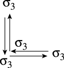
Figure 4: Schematic representation of L-type gauge

4 String Tension

As a first step, we measure abelian and monopole contributions to the string tension in various abelian projections. We used 100 configurations of $32^{3}\times 16$ lattice for the measurement. In this case, the critical point lies near $\beta_{c}\sim 2.7$. We set the gauge coupling $\beta$ to 2.5, so that the system is in the confinement phase. To reduce the statistical errors efficiently, we adopted the hypercubic blocking [26] to the original configurations.

The value of Polyakov loop correlators corresponds to the static potential between one pair of quark and anti-quark;

$$\langle{\mbox{Tr}}P(0){\mbox{Tr}}P^{\dagger}(R)\rangle=e^{-V(R)/T},$$ (18)

where $P(R)$ is the Polyakov loop operator Eq.(14). $V(R)$ gives the inter-quark potential

$$V(R)=\sigma R-\frac{\alpha}{R}+c$$ (19)

and $T=1/(N_{4}a)$ is the temperature of the system.

The abelian Polyakov loop operator is written as

$$P_{a}=\exp[i\sum_{i=0}^{N_{4}-1}\theta_{4}(\vec{s}+i\hat{4})].$$ (20)

Eq.(20) can be decomposed to photon and monopole parts [11] as follows:

$$P_{a} = P_{p}\cdot P_{m},$$

$$P_{p} = \exp[-i\sum_{i=0}^{N_{4}-1}\sum_{s^{\prime}}D(\vec{s}+i\hat{4}-s^{\prime})\partial_{\nu}^{\prime}\bar{\Theta}_{\nu 4}(s^{\prime})],$$

$$P_{m} = \exp[-2\pi i\sum_{i=0}^{N_{4}-1}\sum_{s^{\prime}}D(\vec{s}+i\hat{4}-s^{\prime})\partial_{\nu}^{\prime}n_{\nu 4}(s^{\prime})],$$

where we use an identity

$$\theta_{4}(s)=-\sum_{s^{\prime}}D(s-s^{\prime})\left[\partial_{\nu}^{\prime}\Theta_{\nu 4}(s^{\prime})+\partial_{4}(\partial_{\nu}^{\prime}\theta_{\nu}(s^{\prime}))\right].$$

The abelian field strength tensor

$$\Theta_{\mu\nu}(s)\equiv\theta_{\mu}(s)+\theta_{\nu}(s+\hat{\mu})-\theta_{\mu}(s+\hat{\nu})-\theta_{\nu}(s)\hskip 10.00002pt,\hskip 10.00002pt(-4\pi\leq\theta_{\mu\nu}(s)<4\pi)$$

can be decomposed into two parts:

$$\Theta_{\mu\nu}(s)\equiv\bar{\Theta}_{\mu\nu}(s)+2\pi n_{\mu\nu}(s)\hskip 10.00002pt,\hskip 10.00002pt(-\pi\leq\bar{\Theta}_{\mu\nu}(s)<\pi).$$

Here, $\bar{\Theta}_{\mu\nu}(s)$ is interpreted as the electro-magnetic flux through the plaquette and the integer valued $n_{\mu\nu}(s)$ corresponds to the number of Dirac string piercing the plaquette. $D(s-s^{\prime})$ is the Coulomb propagator on a lattice.

Figures 6, 6, 8 and 8 show the values of $SU(2)$, abelian and monopole Polyakov loop correlators in MA, LA, MAWL and L-type gauges, respectively. The values of abelian and monopole Polyakov loop correlators in each gauge almost degenerate. The string tension $\sigma$ can be extracted from these values by fitting them to Eq.(18). Fitted lines are also plotted in the same figure. In the case of MA gauge, fitted values are consistent with the results by Bali et al [27]. In the case of other gauges like a unitary gauge, one can not extract the string tension clearly from the abelian and the monopole Polyakov loop correlators due to large statistical errors.

Figure 5: Abelian and monopole Polyakov loop correlator in MA gauge

Figure 6: Abelian and monopole Polyakov loop correlator in LA gauge

Figure 7: Abelian and monopole Polyakov loop correlator in MAWL gauge

Figure 8: Abelian and monopole Polyakov loop correlator in L-type gauge

Explicit values of the fitted string tension are shown in Table 1. They almost agree each other, although these four gauges have different gauge fixing condition in the continuum limit.

	MA	LA	MAWL	L-type
Abelian	0.03054(45)	0.03011(34)	0.03051(45)	0.03065(43)
Monopole	0.02545(31)	0.02536(28)	0.02546(31)	0.02624(34)

Table 1: Fitted string tensions ($32^{3}\times 16$ lattice, $\beta=2.5$) $\sigma_{SU(2)}=0.03446(105)$.

5 RG flows of the effective action in various abelian projections

To clarify what is happening in the monopole dynamics, we study the effective monopole actions in various gauges in this section.

5.1 Simulation method

Our method to derive an effective monopole action is the following. We generate $SU(2)$ gauge fields $\{U_{\mu}(s)\}$ using the standard $SU(2)$ Wilson action. We consider $48^{4}$ hypercubic lattice for $\beta$ from 2.1 to 2.5. We took 50 independent configurations after 10,000 thermalization sweeps. Then, we perform the abelian projection in six different gauge fixings to extract abelian gauge fields $\{u_{\mu}(s)\}$ from $SU(2)$ gauge fields.

One can define magnetic monopole currents from abelian field strength tensor along the way of DeGrand and Toussaint [28]. We can define the monopole current $k_{\mu}(s)$ as

$$k_{\mu}(s)=\frac{1}{2}\epsilon_{\mu\nu\rho\sigma}\partial_{\nu}n_{\rho\sigma}(s+\hat{\mu}).$$ (21)

By definition, it satisfies a current conservation law

$$\partial_{\mu}^{\prime}k_{\mu}(s)=0,$$

where $\partial_{\mu}$ and $\partial^{\prime}_{\mu}$ denote the forward and the backward differences in $\mu$-direction respectively.

We want to get an effective monopole action $S[k]$ on the dual lattice, integrating out all degrees of freedom except for monopoles:

$$Z = \int{\cal D}Ue^{-S[U]}\delta(X^{\pm})\Delta_{F}(U)$$

$$= \int{\cal D}u\left[\int{\cal D}Ce^{-S[U]}\delta(X^{\pm})\Delta(U)\right]$$

$$= \int{\cal D}ue^{-S_{eff}[u]}$$

$$= \left(\prod\sum\right)\int{\cal D}ue^{-S_{eff}[u]}\delta(k,f(u))$$

$$= \prod_{s,\mu}\sum_{k_{\mu}(s)=-\infty}^{\infty}\left(\prod_{m,\nu}\delta_{\partial_{\nu}^{\prime}k_{\nu}(m),0}\right)e^{-S[k]},$$

where $U_{\mu}=C_{\mu}u_{\mu}$ and $X^{\pm}$ is the off-diagonal element of the matrix $X$ which is diagonalized in the procedure of abelian projection. $\Delta_{F}(U)$ is the Faddeev-Popov determinant and $\delta(k,f(u))$ gives the definition of the monopole current $k$ as a function of abelian gauge field $u$.

Above integrations are done numerically. We create vacuum ensembles of monopole currents using the Monte-Carlo method and the definition of the monopole current Eq.(21). Then, we construct the effective monopole action from monopole vacua using the Swendsen’s inverse Monte-Carlo method which was developed originally by Swendsen [29] and extended by Shiba and Suzuki [4].

We consider a set of independent and local monopole interactions which are summed up over the whole lattice. We denote each interaction term as $S_{i}[k]$. Then the effective monopole action can be written as a linear combination of these operators:

$$S[k]=\sum_{i}g_{i}S_{i}[k],$$ (22)

where $g_{i}$ denotes the effective coupling constants. Explicit forms of the interaction terms are listed in Table 2 and 3. We determine the set of couplings $\{g_{i}\}$ from the monopole current ensemble $\{k_{\mu}(s)\}$ with the aid of an inverse Monte-Carlo method. Practically, we have to restrict the number of interaction terms. The form of action adopted here is 27 quadratic interactions and 4-point and 6-point interactions [5, 30].

We perform a blockspin transformation in terms of the monopole currents on the dual lattice to study the RG flow. The $n$-step blocked current is defined by

$$K_{\mu}(s^{(n)})=\sum_{i,j,l=0}^{n-1}k_{\mu}(ns^{(n)}+(n-1)\hat{\mu}+i\hat{\nu}+j\hat{\rho}+l\hat{\sigma}).$$ (23)

The blocked lattice spacing $b$ is given as $b=na(\beta)$ and the continuum limit is taken as the limit $n\rightarrow\infty$ for a fixed physical scale $b$. We determine the effective monopole action from the blocked monopole current ensemble $\{K_{\mu}(s^{(n)})\}$. Then one can obtain the RG flow in the 29-dimensional coupling constant space.

Coupling	Distance	Type	Coupling	Distance	Type
$g_{1}$	(0,0,0,0)	$k_{\mu}(s)$	$g_{15}$	(2,1,1,0)	$k_{\mu}(s+2\hat{\mu}+\hat{\nu}+\hat{\rho})$
$g_{2}$	(1,0,0,0)	$k_{\mu}(s+\hat{\mu})$	$g_{16}$	(1,2,1,0)	$k_{\mu}(s+\hat{\mu}+2\hat{\nu}+\hat{\rho})$
$g_{3}$	(0,1,0,0)	$k_{\mu}(s+\hat{\nu})$	$g_{17}$	(0,2,1,1)	$k_{\mu}(s+2\hat{\nu}+\hat{\rho}+\hat{\sigma})$
$g_{4}$	(1,1,0,0)	$k_{\mu}(s+\hat{\mu}+\hat{\nu})$	$g_{18}$	(2,1,1,1)	$k_{\mu}(s+2\hat{\mu}+\hat{\nu}+\hat{\rho}+\hat{\sigma})$
$g_{5}$	(0,1,1,0)	$k_{\mu}(s+\hat{\nu}+\hat{\rho})$	$g_{19}$	(1,2,1,1)	$k_{\mu}(s+\hat{\mu}+2\hat{\nu}+\hat{\rho}+\hat{\sigma})$
$g_{6}$	(2,0,0,0)	$k_{\mu}(s+2\hat{\mu})$	$g_{20}$	(2,2,0,0)	$k_{\mu}(s+2\hat{\mu}+2\hat{\nu})$
$g_{7}$	(0,2,0,0)	$k_{\mu}(s+2\hat{\nu})$	$g_{21}$	(0,2,2,0)	$k_{\mu}(s+2\hat{\nu}+2\hat{\rho})$
$g_{8}$	(1,1,1,1)	$k_{\mu}(s+\hat{\mu}+\hat{\nu}+\hat{\rho}+\hat{\sigma})$	$g_{22}$	(3,0,0,0)	$k_{\mu}(s+3\hat{\mu})$
$g_{9}$	(1,1,1,0)	$k_{\mu}(s+\hat{\mu}+\hat{\nu}+\hat{\rho})$	$g_{23}$	(0,3,0,0)	$k_{\mu}(s+3\hat{\nu})$
$g_{10}$	(0,1,1,1)	$k_{\mu}(s+\hat{\nu}+\hat{\rho}+\hat{\sigma})$	$g_{24}$	(2,2,1,0)	$k_{\mu}(s+2\hat{\mu}+2\hat{\nu}+\hat{\rho})$
$g_{11}$	(2,1,0,0)	$k_{\mu}(s+2\hat{\mu}+\hat{\nu})$	$g_{25}$	(1,2,2,0)	$k_{\mu}(s+\hat{\mu}+2\hat{\nu}+2\hat{\rho})$
$g_{12}$	(1,2,0,0)	$k_{\mu}(s+\hat{\mu}+2\hat{\nu})$	$g_{26}$	(0,2,2,1)	$k_{\mu}(s+2\hat{\nu}+2\hat{\rho}+\hat{\sigma})$
$g_{13}$	(0,2,1,0)	$k_{\mu}(s+2\hat{\nu}+\hat{\rho})$	$g_{27}$	(2,2,1,0)	$k_{\rho}(s+2\hat{\mu}+2\hat{\nu}+\hat{\rho})$
$g_{14}$	(2,1,0,0)	$k_{\nu}(s+2\hat{\mu}+\hat{\nu})$

Table 2: The quadratic interactions used for the modified Swendsen’s method.

Coupling	Type
4-point $g_{28}$	$\quad\quad\sum_{s}\left(\sum_{\mu=-4}^{4}k_{\mu}^{2}(s)\right)^{2}$
6-point $g_{29}$	$\quad\quad\sum_{s}\left(\sum_{\mu=-4}^{4}k_{\mu}^{2}(s)\right)^{3}$

Table 3: The higher order interactions used for the modified Swendsen’s method.

5.2 Numerical Results

The effective monopole action is determined successfully. All coupling constants which are contained in the effective monopole action are obtained with relatively small errors. We use the jackknife method for the error estimation. These effective monopole actions except in MA gauge are determined for the first time in this paper. Moreover, these effective monopole actions are determined from the blocked monopole configurations, too. The results are summarized as follows:

1. Only the quadratic interaction subspace seems sufficient in the coupling space for the low-energy region of QCD. Figure 10 and 10 show coupling constants for 4-point and 6-point interaction terms versus physical scale $b$. In the case of MA, LA, MAWL and L-type gauges, these coupling constants take relatively larger absolute values for small $b$ region. They become negligibly small for large $b$ region. In the case of Polyakov, F₁₂, no gauge fixings, coupling constants for 4-point and 6-point interaction terms take the values very close to zero in the whole region of $b$.

2. Typical case of the coupling constants for quadratic interaction terms versus squared distances in the lattice unit are shown in Figure 11. We see that coupling constants for the self interaction term $g_{1}$ and the nearest-neighbor interactions $g_{2}$ and $g_{3}$ are dominant, and $g_{2}\simeq g_{3}$. Other couplings decrease exponentially as distance between the two monopole currents grows. Such a behavior does not depend on a gauge coupling constant $\beta$. Therefore, we concentrate our analysis on the coupling constants of quadratic interaction terms, especially $g_{1}$ and $g_{2}$.

   

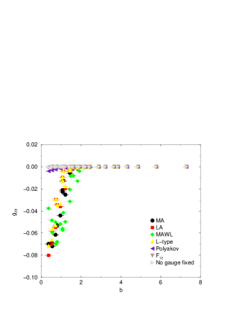
   Figure 9: 4-point coupling $g_{28}$ vs. physical scale $b$.

   

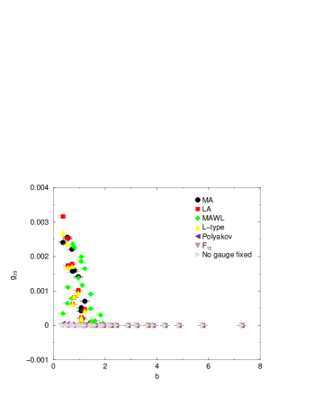
   Figure 10: 6-point coupling $g_{29}$ vs. physical scale $b$.

   

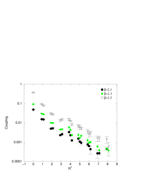
   Figure 11: Effective couplings vs. squared distances in lattice unit. (MA gauge, $\beta=2.1,2.3$ and $2.5$, effective couplings for $n=8$ blocked monopole)

3. We used a standard iterative gauge fixing procedure for MA, MAWL and L-type gauges. In such a case, gauge fixing sweeps may be stuck for some local minima of a gauge fixing functional. Different local minima give rise to different gauge transformations, but they can not be distinguished from the view point of the iterative gauge fixing procedure. These are the lattice Gribov copies. Indeed, Bali et al. showed that the effect of such copies to the abelian string tension is not so small [27]. To check the effect of copies to the effective couplings, we generate 100 of $SU(2)$ configurations on $24^{4}$ lattice at $\beta=2.5$. Then, we generate 7 of gauge equivalent configurations (i.e., copies) via a random gauge transformation. Using these gauge copies, we constructed effective monopole actions and compared their effective couplings. Figure 13 shows $g_{1}$ in the case of MA gauge. $g_{1}$ for the different blocking factors are described in different symbols. We see some fluctuations in $g_{1}$ for MA gauge. This is nothing but the effect of lattice Gribov copies. The effect of the copies, however, are negligibly small. Therefore, qualitative analyses which are given later will not be affected. In principle, LA gauge does not have such a copy [8]. Indeed, we confirmed that effective couplings for LA gauge are not affected by Gribov copies (Figure 13).

   

   Figure 12: Gribov copy effect for $g_{1}$ (MA gauge)

   

   Figure 13: Gribov copy effect for $g_{1}$ (LA gauge)

4. Figure 15 and Figure 15 show the most dominant quadratic self coupling constant $g_{1}$ and quadratic nearest-neighbor coupling constant $g_{2}$ versus physical scale $b$ in the case of MA, LA, MAWL and L-type gauges, respectively. In these gauges, effective coupling constants take large values in small $b$ region and the scaling behavior (i.e., a unique curve for different blocking factor $n$) is seen even in small $b$ region. The effective actions which are obtained here appear to be a good approximation of the action on the renormalized trajectory corresponding to the continuum limit. In addition to this, coupling constants for these four gauges are very close to each other, although these gauges have a completely different form in the continuum limit.

5. However, in the case of Polyakov, F₁₂ and no gauge fixings, coupling constants are different from those in the above four gauges (See, Figure 17 and Figure 17). In these gauges, coupling constants take smaller values and the scaling behavior is not seen especially in small $b$ region. To clarify the scaling properties of these coupling constants, we show the figures as showing a distinction between the different blocking factors $n$ in two typical gauges. In the case of Polyakov gauge (Figure 19), the coupling constants depend on the blocking factor $n$ strongly in small $b$ regions. On the other hand, in the case of LA gauge (Figure 19), renormalized coupling constants are lying on the unique curve.

   

   Figure 14: The most dominant self coupling $g_{1}$ vs. physical scale $b$ in MA, LA, MAWL and L-type gauges.

   

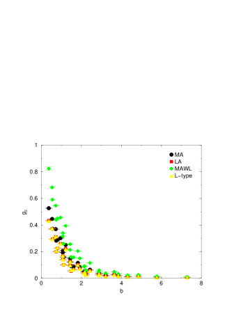
   Figure 15: Nearest-neighbor coupling $g_{2}$ vs. physical $b$ in MA, LA, MAWL and L-type gauges.

   

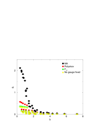
   Figure 16: The most dominant self coupling $g_{1}$ vs. physical scale $b$ in MA, Polyakov, F₁₂ and no gauge fixings.

   

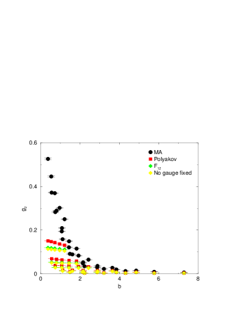
   Figure 17: Nearest-neighbor coupling $g_{2}$ vs. physical scale $b$ in MA, Polyakov, F₁₂ and no gauge fixings.

   

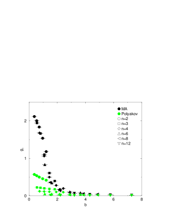
   Figure 18: $g_{1}$ versus $b$ in MA gauge and Polyakov gauge. Each symbols correspond to the different blocking factors $n$.

   

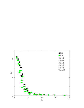
   Figure 19: $g_{1}$ versus $b$ in MA gauge and LA gauge. Each symbols correspond to the different blocking factors $n$.

6. Once the effective actions are fixed, we can see from energy-entropy balance of the system whether monopole condensation occurs or not. If the entropy of a monopole loop exceeds the energy, the monopole loop condenses in the QCD vacuum. In four-dimensional lattice theory, the entropy of a monopole loop can be estimated as $\ln 7$ per unit loop length. It is determined by the random walk without backward tracking. The action can be approximated by the self interaction term $g_{1}$ alone since the interactions with two separate currents are almost canceled [31]. The free energy per unit monopole length is approximated by

   $$F\sim g_{1}-\ln 7,$$

   since $g_{1}$ can be regarded as the self energy per unit monopole loop length. If $g_{1}<\ln 7$, the entropy dominates over the energy, that is, monopole condensation occurs. In Figure 15 and Figure 17, we see that the entropy of the system dominates over the energy in the large $b$ region for all gauges. In other words, monopole condensation occurs [4] in the large $b$ region for all gauges.

7. Figures 21,21,23 and 23 show the RG flows projected onto $g_{1}$-$g_{2}$, $g_{1}$-$g_{5}$, $g_{1}$-$g_{7}$ and $g_{1}$-$g_{10}$ coupling planes, respectively. The effective coupling constants for all gauges seem to converge to the identical line for large $b$ region. This may show gauge independence of the monopole condensation in the low energy region. Although all coupling constants become very small in the large $b$ region, it is important that the slopes of the renormalization flows seem to converge in all gauges.

   

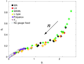
   Figure 20: RG flows of the effective monopole actions project onto the $g_{1}$-$g_{2}$ coupling plane

   

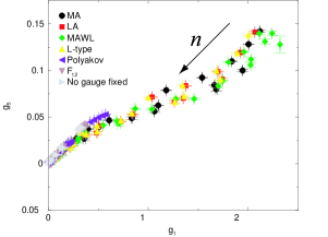
   Figure 21: RG flows of the effective monopole actions project onto the $g_{1}$-$g_{5}$ coupling plane

   

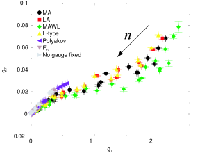
   Figure 22: RG flows of the effective monopole actions project onto the $g_{1}$-$g_{7}$ coupling plane

   

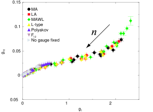
   Figure 23: RG flows of the effective monopole actions project onto the $g_{1}$-$g_{10}$ coupling plane

6 Summary

We have measured first the abelian and the monopole contributions to the string tension in four types of abelian projections, i.e., MA, LA, MAWL and L-type gauges. They show a good agreement with each other. Monopole string tension are extracted in the same manner as abelian string tension, and they agree also with each other. MA and LA gauges are not unique good gauges.

Next, we have determined the effective monopole actions in various gauges from monopole vacua using the modified Swendsen’s method. In the case of MA gauge, an effective monopole action has already been obtained in Ref. [4]. In addition to this action, the effective monopole actions in Polyakov gauge, F₁₂ gauge, LA gauge, MAWL gauge, L-type gauge and no gauge fixing are also determined for the first time in this paper. Moreover, these effective actions are determined on the blocked monopole vacua, too. In these effective actions, two point interactions are dominant, whereas 4-point and 6-point effective coupling constants are negligibly small in the infrared region. The RG flows seem to converge to the identical line when repeating the blockspin transformation. It is important that the slopes of renormalization flows in all gauges seem to converge. The data are compatible with the assumption of gauge independence of monopole dynamics in the continuum limit. Energy-entropy balance also tells us the monopole condensation occurs in the large $b$ region for all gauges.

Appendix A Maximally Abelian Wilson Loop (MAWL) gauge

$SU(2)$ gauge field $U_{\mu}(s)$ can be parameterized by its isospin components. In this section, we denote each isospin component of $U_{\mu}(s)$ as $U_{0}(s,\mu)$, $U_{1}(s,\mu)$ and so on, for simplicity. This gauge is realized with maximizing the abelian Wilson loop of $1\times 1$ size:

$$R=\sum_{s,\mu\neq\nu}\cos\Theta_{\mu\nu}(s),$$ (24)

where the abelian link field is extracted as

$$\theta(s,\mu)=\arctan(U_{3}(s,\mu)/U_{0}(s,\mu)).$$ (25)

Let us consider an infinitesimal gauge transformation of $U$,

$$U^{\prime}(s,\mu)=(1+i\alpha_{i}(s)\sigma_{i})(U_{0}(s,\mu)I+iU_{j}(s,\mu)\sigma_{j})(1-i\alpha_{k}(s+\hat{\mu})\sigma_{k}).$$ (26)

This gives

$$\delta U_{0}(s,\mu) = -(\alpha_{i}(s)-\alpha_{i}(s+\hat{\mu}))U_{i}(s,\mu),$$ (27)

$$\delta U_{k}(s,\mu) = (\alpha_{k}(s)-\alpha_{k}(s+\hat{\mu}))U_{0}(s,\mu)-\epsilon_{ijk}(\alpha_{i}(s)+\alpha_{i}(s+\hat{\mu}))U_{j}(s,\mu).$$ (28)

Then $R$ changes as

$$\delta R=-\sum_{s,\mu\neq\nu}\sin\Theta_{\mu\nu}(s)(\delta\theta(s,\mu)+\delta\theta(s+\hat{\mu},\nu)-\delta\theta(s+\hat{\mu},\mu)-\delta\theta(s,\nu)),$$ (29)

where

$$\delta\theta(s,\mu)=\frac{U_{0}(s,\mu)\delta U_{3}(s,\mu)-U_{3}(s,\mu)\delta U_{0}(s,\mu)}{U_{0}^{2}(s,\mu)+U_{3}^{2}(s,\mu)}.$$ (30)

One can check that $R$ is invariant under the $U(1)$ transformation. Hence we do not need to consider the $\alpha_{3}(s)$ part. First, let us consider the $\alpha_{1}$ part. Since there is the sum over whole lattice sites $s$, one can shift the site variable, for example, $s$ to $s-\hat{\mu}$. Also one can use the (anti)symmetric property with respect to $\mu$ and $\nu$ directions. Finally one gets,

$$-\frac{\delta R}{2} = \sum_{s,\mu\neq\nu}(\alpha_{1}(s)X_{1}(s,\mu,\nu)+\alpha_{2}(s)X_{2}(s,\mu,\nu)),$$

$$X_{1}(s,\mu,\nu) = W_{1}\frac{U_{1}(s,\mu)U_{3}(s,\mu)-U_{0}(s,\mu)U_{2}(s,\mu)}{U_{0}^{2}(s,\mu)+U_{3}^{2}(s,\mu)}$$

$$+W_{2}\frac{U_{1}(s-\hat{\mu},\mu)U_{3}(s-\hat{\mu},\mu)+U_{0}(s-\hat{\mu},\mu)U_{2}(s-\hat{\mu},\mu)}{U_{0}^{2}(s-\hat{\mu},\mu)+U_{3}^{2}(s-\hat{\mu},\mu)},$$

$$X_{2}(s,\mu,\nu) = W_{1}\frac{U_{2}(s,\mu)U_{3}(s,\mu)+U_{0}(s,\mu)U_{1}(s,\mu)}{U_{0}^{2}(s,\mu)+U_{3}^{2}(s,\mu)}$$

$$+W_{2}\frac{U_{2}(s-\hat{\mu},\mu)U_{3}(s-\hat{\mu},\mu)-U_{0}(s-\hat{\mu},\mu)U_{1}(s-\hat{\mu},\mu)}{U_{0}^{2}(s-\hat{\mu},\mu)+U_{3}^{2}(s-\hat{\mu},\mu)},$$

$$W_{1} = \sin\Theta_{\mu\nu}(s)-\sin\Theta_{\mu\nu}(s-\hat{\nu}),$$

$$W_{2} = \sin\Theta_{\mu\nu}(s-\hat{\mu}-\hat{\nu})-\sin\Theta_{\mu\nu}(s-\hat{\mu}).$$

When we write $X^{\pm}=X_{1}\pm iX_{2}$, it is easy to see $X^{\pm}$ transforms covariantly under the residual $U(1)$.

Finally, one gets the matrix which is diagonalized in this gauge,

$$X(s) = \sum_{\mu\neq\nu}\left[\frac{\sin\Theta_{\mu\nu}(s)-\sin\Theta_{\mu\nu}(s-\hat{\nu})}{U_{0}^{2}(s,\mu)+U_{3}^{2}(s,\mu)}(U(s,\mu)\sigma_{3}U^{\dagger}(s,\mu))\right.$$

$$+\left.\frac{\sin\Theta_{\mu\nu}(s-\hat{\mu}-\hat{\nu})-\sin\Theta_{\mu\nu}(s-\hat{\mu})}{U_{0}^{2}(s-\hat{\mu},\mu)+U_{3}^{2}(s-\hat{\mu},\mu)}(U^{\dagger}(s-\hat{\mu},\mu)\sigma_{3}U(s-\hat{\mu},\mu))\right].$$

Because of the non-locality of the gauge condition, one can not calculate the gauge transformation matrix which diagonalizes $X(s)$ in a simple way. Therefore, we employed an iterative updation procedure to satisfy the gauge condition.

1. Make a trial gauge transformation, adopting $\alpha_{1}$ and $\alpha_{2}$ as follows:
   $\alpha_{1}(s)=-\kappa X_{1}(s)$,
   $\alpha_{2}(s)=-\kappa X_{2}(s)$.

2. Measure $R$. If $R$ becomes larger than before, accept this trial and repeat step 1. If $R$ becomes smaller than before, take $\kappa_{new}=\kappa_{old}/2$ and adopt the gauge transformation using this $\kappa_{new}$ with respect to the configuration before trial, and then repeat step 1.

3. If the off-diagonal element of $X(s)$ becomes smaller than a suitable threshold (we set this to $1.0$), one can regard the gauge fixing procedure as having been completed.

We set an initial value of $\kappa$ to $0.1$. $R$ can be maximized as long as we take $\kappa>0$. We apply the MA gauge fixing as a preconditioning for MAWL gauge fixing and then we perform the above procedure to the MA fixed configuration. This preconditioning is required to improve a convergence property of the MAWL gauge fixing. We have to note that the configurations which obtained via the above procedure are not perfectly gauge fixed because the off-diagonal element of $X(s)$ still remain not very small.

References

- [1] G. ’t Hooft: in High Energy Physics, ed. A. Zichichi (Editorice Compositori Bologna, 1976)
- [2] S. Mandelstam: Phys. Rept. 23C (1976) 245
- [3] G. ’t Hooft, Nucl. Phys. B 190 (1981) 455
- [4] H. Shiba and T. Suzuki, Phys. Lett. B 343 (1995) 315 ; Phys. Lett. B 351 (1995) 519 and references there in.
- [5] M. N. Chernodub et al., Phys. Rev. D 62 (2000) 094506
- [6] Gunnar S. Bali, Christoph Schlichter, Klaus Schilling: Prog. Theor. Phys. Suppl. 131 (1998) 645-656
- [7] Y. Koma, E. -M. Ilgenfritz, T. Suzuki, H. Toki: Phys. Rev. D 64 (2001) 014015
- [8] A. J. van der Sijs, Prog. Theor. Phys. Suppl. 131 (1998) 149-159
- [9] A. J. van der Sijs, Nucl. Phys. 73 (Proc. Suppl.) (1999) 548-550
- [10] T. Suzuki and I. Yotsuyanagi, Phys. Rev. D 42 (1990) 4257, Nucl. Phys. B20 (Proc. Suppl.) (1991) 236.
- [11] Shinji Ejiri, Shun-ichi Kitahara, Yoshimi Matsubara, Tsuyoshi Okude, Tsuneo Suzuki, Koji Yasuta, Nucl. Phys. 47 (Proc. Suppl.) (1996) 322-325
- [12] F. Shoji, T. Suzuki, H. Kodama, A. Nakamura, Phys. Lett. B 476 (2000) 199-204
- [13] Tsuneo Suzuki, Sawut Ilyar, Yoshimi Matsubara, Tsuyoshi Okude, Kenji Yotsuji, Phys. Lett. B 347 (1995) 375-380; Erratum-ibid. B351 (1995) 603
- [14] M. C. Ogilvie, Phys. Rev. D 59 (1999) 074505
- [15] John D. Stack, Steven D. Neiman, Roy J. Wensley, Phys. Rev. D 50 (1994) 3399-3405
- [16] H. Shiba and T. Suzuki, Phys. Lett. B 333 (1994) 461-466
- [17] K. Yamagishi, S. Kitahara, S. Ito, T. Tsunemi, S. Fujimoto, S. Kato, F. Shoji, T. Suzuki, H. Kodama, A. Nakamura, Nucl. Phys. 83 (Proc. Suppl.) (2000) 550-552
- [18] V. L. Beresinskii: Sov. Phys. JETP 32 (1970) 493.
- [19] J. M. Kosterlitz and D.J. Thouless, J. Phys. C 6 (1973) 1181.
- [20] A. Di Giacomo: hep-lat/0206018 and references therein.
- [21] O. Jahn, F. Lenz: Phys. Rev. D 58 (1998) 085006
- [22] M. N. Chernodub, F.V. Gubarev, M.I. Polikarpov, A.I. Veselov: Prog. Theor. Phys. Suppl. 131 (1998) 309-321
- [23] Shinji Ejiri, Shun-ichi Kitahara, Yoshimi Matsubara, Tsuneo Suzuki, Phys. Lett. B 343 (1995) 304-309
- [24] See, http://www.caam.rice.edu/software/ARPACK/
- [25] Tsuneo Suzuki, Yoshimi Matsubara, Shun-ichi Kitahara, Shinji Ejiri, Naoki Nakamura, Fumiyoshi Shoji, Masafumi Sei, Seikou Kato, Natsuko Arasaki, Nucl. Phys. 53 (Proc. Suppl.) (1997) 531-534
- [26] A. Hasenfratz, F. Knechtli: Phys. Rev. D 64 (2001) 034504
- [27] G. S. Bali, V. Bornyakov, M. Mueller Preussker, K. Schilling: Phys. Rev. D 54 (1996) 2863-2875
- [28] T. A. DeGrand and D. Toussaint, Phys. Rev. D 22 (1980) 2478.
- [29] R. H. Swendsen, Phys. Rev. Lett. 52 (1984) 1165 ; Phys. Rev. B 30 (1984) 3866,3875.
- [30] Maxim N. Chernodub, Seikou Kato, Naoki Nakamura, Mikhail I. Polikarpov, Tsuneo Suzuki: hep-lat/9902013
- [31] Shun-ichi Kitahara, Yoshimi Matsubara, Tsuneo Suzuki: Prog. Theor. Phys. 93 (1995) 1