Gluon Propagator on Coarse Lattices in Laplacian Gauges

Abstract

The Laplacian gauge is a nonperturbative gauge fixing that reduces to Landau gauge in the asymptotic limit. Like Landau gauge, it respects Lorentz invariance, but it is free of Gribov copies; the gauge fixing is unambiguous. In this paper we study the infrared behavior of the lattice gluon propagator in Laplacian gauge by using a variety of lattices with spacings from $a=0.125$ to 0.35 fm, to explore finite volume and discretization effects. Three different implementations of the Laplacian gauge are defined and compared. The Laplacian gauge propagator has already been claimed to be insensitive to finite volume effects and this is tested on lattices with large volumes.

I Introduction

The lattice provides a useful tool for studying the gluon propagator because it is a first principles treatment that can, in principle, access any momentum window. There is tremendous interest in the infrared behavior of the gluon propagator as a probe into the mechanism of confinement background and lattice studies focusing on its ultraviolet behavior have been used to calculate the running QCD coupling Bec99 . Such studies can also inform model hadron calculations models . Although there has recently been interest in Coulomb gauge Cuc01 and generic covariant gauges Giu01 , the usual gauge for these studies has been Landau gauge, because it is a (lattice) Lorentz covariant gauge that is easy to implement on the lattice, and its popularity means that results from the lattice can be easily compared to studies that use different methods. Finite volume effects and discretization errors have been extensively explored in lattice Landau gauge Lei99 ; Bon00 ; Bon01 . Unfortunately, lattice Landau gauge suffers from the well-known problem of Gribov copies. Although the ambiguity originally noticed by Gribov Gri78 is not present on the lattice, the maximization procedure used for gauge fixing does not uniquely fix the gauge. There are, in general, many local maxima for the algorithm to choose from, each one corresponding to a Gribov copy, and no local algorithm can choose the global maximum from among them. While various remedies have been proposed Het98 ; evolutionary , they are either unsatisfactory or computationally very intensive. For a recent discussion of the Gribov problem in lattice gauge theory, see Ref. Wil02 .

An alternative approach is to operate in the so-called Laplacian gauge Vin92 . This gauge is “Landau like” in that it has similar smoothness and Lorentz invariance properties Vin95 , but it involves a non-local gauge fixing procedure that avoids lattice Gribov copies. Laplacian gauge fixing also has the virtue of being rather faster than Landau gauge fixing on the lattice. The gluon propagator has already been studied in Laplacian gauge in Refs. Ale01 ; Ale02 and the improved staggered quark propagator in Laplacian gauge in Ref. quarkprop .

In this report we explore three implementations of the Laplacian gauge and their application to the gluon propagator on coarse, large lattices, using an improved action as has been done for Landau gauge in Ref. Bon01 . We study the gluon propagator in quenched QCD (pure $SU(3)$ Yang-Mills), using an ${\cal O}(a^{2})$ mean-field improved gauge action. To assess the effects of finite lattice spacing, we calculate the propagator on a set of lattices from $10^{3}\times 20$ at $\beta=3.92$ having $a=0.353$ fm to $16^{3}\times 32$ at $\beta=4.60$ having $a=0.125$ fm. To assist us in observing possible finite volume effects, we add to this set a $16^{3}\times 32$ lattice at $\beta=3.92$ with $a=0.353$, which has the very large physical size of $5.65^{3}\times 11.30\text{ fm}^{4}$.

The infrared behavior of the Laplacian gauge gluon propagator is found to be qualitatively similar to that seen in Landau gauge. Like Refs. Ale01 ; Ale02 , little volume dependence is seen in the propagator, but, unlike Landau gauge, the Laplacian gauge displays strong sensitivity to lattice spacing, making large volume simulations difficult. We conclude that further work involving an improved gauge fixing is desired.

II The Laplacian Gauges

Laplacian gauge is a nonlinear gauge fixing that respects rotational invariance, has been seen to be smooth, yet is free of Gribov ambiguity. It reduces to Landau gauge in the asymptotic limit, yet is computationally cheaper than Landau gauge. There is, however, more than one way of obtaining such a gauge fixing in $SU(N)$. The three implementations of Laplacian gauge fixing discussed are

1. $\partial^{2}\text{(I)}$ gauge (QR decomposition), used by Alexandrou et al. in Ref. Ale01 .

2. $\partial^{2}\text{(II)}$ gauge (Maximum trace), where the Laplacian gauge transformation is projected onto $SU(3)$ by maximizing its trace. Also used in Ref. quarkprop .

3. $\partial^{2}\text{(III)}$ gauge (Polar decomposition), the original prescription described in Ref. Vin92 and tested in Ref. Vin95 .

All three versions reduce to the same gauge in $SU(2)$.

The gauge transformations employed in Laplacian gauge fixing are constructed from the lowest eigenvectors of the covariant lattice Laplacian

$$\sum_{y}\sum_{j}\Delta(U)(x,y)^{ij}v(y)_{j}^{s}=\lambda^{s}v(x)_{i}^{s},$$ (1)

where

$$\Delta(U)(x,y)^{ij}\equiv\sum_{\mu}\bigl{[}2\delta(x-y)\delta^{ij}-U_{\mu}(x)^{ij}\delta(x+\hat{\mu}-y)-U_{\mu}(y)^{\dagger ij}\delta(y+\hat{\mu}-x)\bigr{]},$$ (2)

$i,j=1,\ldots,N$ for $SU(N)$ and $s$ labels the eigenvalues and eigenvectors. Under gauge transformations of the gauge field,

$$U_{\mu}(x)\rightarrow U_{\mu}^{G}(x)=G(x)U_{\mu}(x)G^{\dagger}(x+\mu),$$ (3)

the eigenvectors of the covariant Laplacian transform as

$$v(x)^{s}\rightarrow G(x)v(x)^{s}$$ (4)

and this property enables us to construct a gauge fixing that is independent of our starting place in the orbit of gauge equivalent configurations.

The three implementations discussed differ in the way that the gauge transformation is constructed from the above eigenvectors. In all cases the resulting gauge should be unambiguous so long as the Nth and (N+1)th eigenvectors are not degenerate and the eigenvectors can be satisfactorily projected onto $SU(N)$. A complex $2\times 2$ matrix can be uniquely projected onto $SU(2)$, but this is not the case for $SU(N)$. Here we can think of the projection method as defining its own, unambiguous, Laplacian gauge fixing.

In the original formulation Vin92 , which we shall rather perversely refer to as $\partial^{2}\text{(III)}$, the lowest $N$ eigenvectors are required to gauge fix an $SU(N)$ gauge theory. These form the columns of a complex $N\times N$ matrix,

$$M(x)^{ij}\equiv v(x)_{i}^{j}$$ (5)

which is then projected onto $SU(N)$ by polar decomposition. Specifically, it is possible to express $M$ in terms of a unitary matrix and a positive hermitian matrix: $M=UP$. This decomposition is unique if $P=(M^{\dagger}M)^{1/2}$ is invertible, which will be true if $M$ is non-singular, i.e., if the eigenvectors used to construct $M$ are linearly independent. The gauge transformation $G(x)$ is then obtained by factoring out the determinant of the unitary matrix

$$G^{\dagger}(x)=U(x)/\det[U(x)].$$ (6)

The gauge transformation $G(x)$ obtained in this way is used to transform the gauge field (i.e., the links) to give the Laplacian gauge-fixed gauge field. $G(x)$ can be uniquely defined by this presciption except on a set of gauge orbits with measure zero (with respect to the the gauge-field functional intregral). Note that if we perform a random gauge transformation $G_{r}(x)$ on the initial gauge field used to define our Laplacian operator, then we will have $v(x)^{s}\to v^{\prime}(x)^{s}=G_{r}(x)v(x)^{s}$ and $M(x)\to M^{\prime}(x)=G_{r}(x)M(x)$. We see that $P\equiv(M^{\dagger}M)^{1/2}\to P^{\prime}=P$ and hence $G(x)\to G^{\prime}(x)=G(x)G^{\dagger}_{r}(x)$. When this is applied to the transformed gauge field it will be taken to exactly the same point on the gauge orbit as the original gauge field went to when gauge fixed. Thus all points on the gauge orbit will be mapped to the same single point on the gauge orbit after Laplacian gauge fixing and so it is a complete (i.e., Gribov-copy free) gauge fixing. This method was investigated for $U(1)$ and $SU(2)$ Vin95 . It is clear that any prescription for projecting $M$ onto some $G^{\dagger}(x)$, which preserves the property $G(x)\to G^{\prime}(x)=G(x)G^{\dagger}_{r}(x)$ under an arbitrary gauge transformation $G_{r}(x)$, will also be a Gribov-copy free Laplacian gauge fixing. Every different projection method with this property is an equally valid but distinct form of Laplacian gauge fixing.

The next approach was used in Ref. Ale01 , and we shall refer to it as $\partial^{2}\text{(I)}$ gauge. There it was noted that only $N-1$ eigenvectors are actually required. To be concrete, we discuss $N=3$. First, apply a gauge transformation, $G(x)^{1}$, to the first eigenvector such that

$$\bigl{[}G(x)^{1}v(x)^{1}\bigr{]}_{1}=||v(x)^{1}||$$ (7)

and

$$\bigl{[}G(x)^{1}v(x)^{1}\bigr{]}_{2}=\bigl{[}G(x)^{1}v(x)^{1}\bigr{]}_{3}=0,$$ (8)

where subscripts label the vector elements, i.e., the eigenvector - with dimension 3 - is rotated so that its magnitude is entirely in its first element. Another gauge transformation, $G(x)^{2}$, rotates the second eigenvector, $v(x)^{2}$, such that

$$\bigl{[}G(x)^{2}v(x)^{2}\bigr{]}_{2}=\sqrt{(v_{2}^{2})^{2}+(v_{3}^{2})^{2}},$$ (9)

and

$$\bigl{[}G(x)^{2}v(x)^{2}\bigr{]}_{3}=0.$$ (10)

This second rotation is an $SU(2)$ subgroup, which does not act on $v_{1}^{2}(x)$. The gauge fixing transformation is then $G(x)=G(x)^{2}G(x)^{1}$. Compare this to QR decomposition, where a matrix, $A$, is rewritten as the product of an orthogonal matrix and an upper triangular matrix. The gauge transformations are thus like Householder transformations.

In addition, we explore a third version, $\partial^{2}\text{(II)}$gauge, where $G(x)$ is obtained by projecting $M(x)$ onto $SU(N)$ by trace maximization. $M(x)$ is again composed of the $N$ lowest eigenvectors and the trace of $G(x)M(x)^{\dagger}$ is maximized by iteration over Cabbibo-Marinari subgroups.

III The Gluon Propagator in Laplacian Gauge

We extract the gluon field from the lattice links by

$$A_{\mu}(x+\hat{\mu}/2)=\frac{1}{2ig_{0}u_{0}}\bigl{\{}U_{\mu}(x)-U_{\mu}^{\dagger}(x)\bigr{\}}_{\text{traceless}},$$ (11)

which differs from the continuum field by terms of ${\cal O}(a^{2})$. $A_{\mu}$ is then transformed into momentum space,

$$A_{\mu}(\hat{q})=\frac{1}{V}\sum_{x}e^{-i\hat{q}\cdot(x+\hat{\mu}/2)}A_{\mu}(x+\hat{\mu}/2),$$ (12)

where the available momenta, $\hat{q}$, are given by

$$\hat{q}_{\mu}=\frac{2\pi n_{\mu}}{aL_{\mu}},\qquad n_{\mu}\in\Bigl{(}-\frac{L_{\mu}}{2},\frac{L_{\mu}}{2}\Bigr{]}.$$ (13)

$L_{\mu}$ is the number of lattice sites in the $\mu$ direction. The momentum space gluon propagator is then

$$D_{\mu\nu}^{ab}(\hat{q})=\langle A_{\mu}^{a}(-\hat{q})A_{\nu}^{b}(\hat{q})\rangle.$$ (14)

Note that this definition includes a factor of $u_{0}^{-2}$ from Eq. (11); this is the same normalization that was used in Ref. Bon01 .

In the continuum, the gluon propagator has the tensor structure

$$D_{\mu\nu}^{ab}(q)=\bigl{(}\delta_{\mu\nu}-\frac{q_{\mu}q_{\nu}}{q^{2}}\bigl{)}\delta^{ab}D(q^{2})+\frac{q_{\mu}q_{\nu}}{q^{2}}\delta^{ab}F(q^{2}).$$ (15)

In Landau gauge the longitudinal part will be zero for all $q^{2}$, but this will not be the case in Laplacian gauge. We note that

$$\frac{q_{\mu}D_{\mu\nu}^{ab}(q)q_{\nu}}{q^{2}}=\delta^{ab}F(q^{2})$$ (16)

and use this to project out the longitudinal part. This, unfortunately, makes it impossible to directly measure the scalar propagator at zero four-momentum, $D(0)$. We are, however, able to measure the full propagator, $\mathcal{D}(0)$. In a covariant gauge $F(q^{2})\rightarrow\frac{\xi_{0}}{q^{2}}$ where $\xi_{0}$ is the bare gauge fixing parameter.

On the lattice the bare propagator is measured, which is related to the renormalized propagator by,

$$D(q^{2})=Z_{3}(\mu)\widetilde{D}(q^{2};\mu^{2})\qquad F(q^{2})=Z_{3}(\mu)\widetilde{F}(q^{2};\mu^{2})$$ (17)

where $\mu$ is the renormalization point. In a renormalizable theory such as QCD, the renormalized quantities become independent of the regularization parameter in the limit where it is removed. $Z_{3}$ is then defined by some renormalization prescription, such as the off-shell subtraction (MOM) scheme, where the renormalized propagator is required to satisfy,

$$\widetilde{D}(\mu^{2})=\frac{1}{\mu^{2}}.$$ (18)

It follows that

$$q^{2}D(q)|_{q^{2}=\mu^{2}}=Z_{3}(\mu;a).$$ (19)

With covariant gauge fixing, the longitudinal part is usually treated by absorbing the renormalization into the gauge parameter, $\xi_{0}=Z_{3}\xi$. We shall not discuss the renormalized propagator in this paper, but only consider relative normalizations for the purpose of comparing different data sets.

	Dimensions	$\beta$	$a\text{ (fm)}$	Volume $\text{(fm}^{4}\text{)}$	Configurations
1	$12^{3}\times 24$	4.60	0.125	$1.50^{3}\times 3.00$	100
2i	$16^{3}\times 32$	4.60	0.125	$2.00^{3}\times 4.00$	100
2w	$16^{3}\times 32$	5.85	0.130	$2.08^{3}\times 4.16$	80
3	$16^{3}\times 32$	4.38	0.166	$2.64^{3}\times 5.28$	100
4	$12^{3}\times 24$	4.10	0.270	$3.24^{3}\times 6.48$	100
5	$10^{3}\times 20$	3.92	0.353	$3.53^{3}\times 7.06$	100
6	$16^{3}\times 32$	3.92	0.353	$5.65^{3}\times 11.30$	89

Table 1: Details of the lattices used to calculate the gluon propagator. Lattice 2w was generated with the Wilson gauge action.

The ensembles studied are listed in Table 1. To help us explore lattice artifacts, some of the following figures will distinguish data on the basis of its momentum components. Data points that come from momenta lying entirely along a spatial Cartesian direction are indicated with a square while points from momenta entirely in the temporal direction are marked with a triangle. As the time direction is longer than the spatial directions any difference between squares and triangles may indicate that the propagator is affected by the finite volume of the lattice. Data points from momenta entirely on the four-diagonal are marked with a diamond. A systematic separation of data points taken on the diagonal from those in other directions indicates a violation of rotational symmetry.

In the continuum, the scalar function is rotationally invariant. Although the hypercubic lattice breaks O(4) invariance, it does preserve the subgroup of discrete rotations Z(4). In our case, this symmetry is reduced to Z(3) as one dimension will be twice as long as the other three in each of the cases studied. We exploit this discrete rotational symmetry to improve statistics through Z(3) averaging Lei99 ; Bon01 .

As has become standard practice in lattice gluon propagator studies, we select our lattice momentum in accordance with the tree-level behavior of the action. With this improved action,

$$q_{\mu}=\frac{2}{a}\sqrt{\sin^{2}\Bigl{(}\frac{\hat{q}_{\mu}a}{2}\Bigr{)}+\frac{1}{3}\sin^{4}\Bigl{(}\frac{\hat{q}_{\mu}a}{2}\Bigr{)}};$$ (20)

this is discussed in more detail in Ref. Bon01 .

IV Results

IV.1 Finer lattices

We start by checking that our finest lattice, at $a=0.125$ fm, is “fine enough”, by comparing the propagator with that of Alexandrou et al. Ale01 . Fig. 1 shows the momentum-enhanced propagator, $q^{2}\,D(q^{2})$, in $\partial^{2}\text{(I)}$ gauge for ensemble 2i (improved action) compared to the data from Ref. Ale01 for the Wilson action at $\beta=6.0$. The two are in excellent agreement.

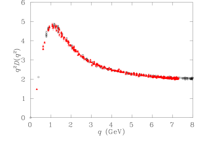
Figure 1: The momentum-enhanced propagator in $\partial^{2}\text{(I)}$ gauge for the Wilson gauge action at $\beta=6.0$ (open circles; data from Ref. Ale01 ) and the improved gauge action at $\beta=4.60$ (filled triangles). Both lattices are $16^{3}\times 32$. Data has been cylinder cut. The two are in excellent agreement. In Ref. Bon01 the difference in normalization between the Wilson and improved actions was seen to be $\sim 1.08$. After taking this into account, the relative normalization here is $Z_{3}(\beta=4.60)=1.07Z_{3}(\beta=6.0)$

.

As the gluon propagator has been extensively studied in Landau gauge, it makes sense to understand the Laplacian gauge propagator by comparing it to that in Landau gauge. In accordance with custom, we will discuss the momentum-enhanced propagator, $q^{2}D(q)$. We define the relative $Z_{3}$ renormalization constant

$$Z_{R}\equiv\frac{Z_{3}(\text{Landau})}{Z_{3}(\text{Laplacian})},$$ (21)

and choose to perform this matching at $\mu=4.0$ GeV. The purpose of this is simply to make the (bare) gluon propagators agree in the ultraviolet for easy comparison between the gauges.

We show the gluon propagator in both Landau and $\partial^{2}\text{(II)}$ gauges in Fig. 2. In this figure, the data is for the largest finer lattices, 2i and 3. The data has been cylinder cut Lei99 ; Bon01 to make comparison easier.

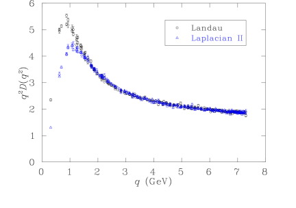
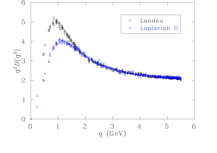
Figure 2: Comparison of the gluon propagator in Landau and $\partial^{2}\text{(II)}$ gauges for lattice 2i (top) and 3 (bottom) ($16^{3}\times 32$, improved action, $\beta=4.60$ and 4.38 respectively). Data has been cylinder cut. The relative normalizations are $Z_{R}(\beta=4.60)=1.075$ and $Z_{R}(\beta=4.38)=1.20$.

As was seen in Ref. Ale01 ; Ale02 , the gluon propagator in Laplacian gauge looks very similar to the Landau gauge case matching up in the ultraviolet but with a somewhat lower infrared hump.

Having compared the gluon propagator in $\partial^{2}\text{(II)}$ gauge to Landau gauge, we now compare it to other implementations of the Laplacian gauge. We expect each implementation to provide a well defined, unambiguous, but different gauge. As we saw when comparing Landau and $\partial^{2}\text{(II)}$ gauges, there is some difference in normalization between the propagators in the different gauges, so we define, again at $\mu=4.0$ GeV

$$Z_{\partial}=\frac{Z_{3}(\partial^{2}\text{(II)})}{Z_{3}(\partial^{2}\text{(I)})}.$$ (22)

In Fig. 3, the momentum-enhanced propagator is plotted in $\partial^{2}\text{(I)}$ and $\partial^{2}\text{(II)}$ gauges for one of the fine lattices (ensemble 2i). There is a small relative normalization ($Z_{\partial}=0.98$), but otherwise there is no significant difference between them, neither in the ultraviolet nor the infrared. $\partial^{2}\text{(I)}$ and $\partial^{2}\text{(II)}$ also show comparable performance in terms of rotational symmetry.

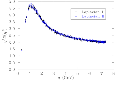
Figure 3: The momentum-enhanced propagator from ensemble 2i ($\beta=4.60,16^{3}\times 32$, improved action) in $\partial^{2}\text{(I)}$ and $\partial^{2}\text{(II)}$ gauges. Data has been cylinder cut. The two gauges produce nearly identical gluon propagators, up to a small relative normalization ($Z_{\partial}=0.98$).

One difference between Landau and Laplacian gauge is that in the former, the gluon propagator has no longitudinal component. We see in Fig. 4 that the longitudinal part of the propagator does indeed vanish in the ultraviolet, which is consistent with approaching Landau gauge, but gains strength in the infrared. Comparing $\partial^{2}\text{(I)}$ and $\partial^{2}\text{(II)}$ gauges we note that while the transverse parts look alike, the longitudinal behavior is quite distinct. The separation of squares and triangles in $\partial^{2}\text{(II)}$ gauge suggests that $F(q^{2})$ has stronger volume dependence in that gauge. For a comparison between Landau, $\partial^{2}\text{(I)}$ and $\partial^{2}\text{(II)}$ gauges for the quark propagator see Ref. quarkprop .

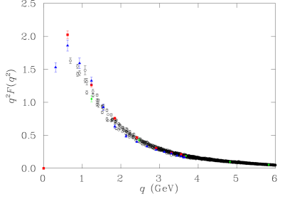
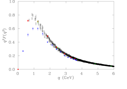
Figure 4: Comparison of the longitudinal part of the gluon propagator in $\partial^{2}\text{(I)}$ (above) and $\partial^{2}\text{(II)}$ (below) gauges for lattice 2i ($\beta=4.60,16^{3}\times 32$, improved action). There have been no data cuts or renormalization. Note that the vertical scales are different, so the longitudinal component is smaller in $\partial^{2}\text{(II)}$ gauge than $\partial^{2}\text{(I)}$. The data has been sorted into points where all the momentum is in the temporal direction, spatial cartestian direction, four-diagonal, and the rest. The separation of temporal points (triangles) from spatial cartesian points (squares) suggests that this part of the gluon propagator has stronger volume dependence in $\partial^{2}\text{(II)}$ gauge than in $\partial^{2}\text{(I)}$ gauge. In a standard covariant gauge this would be a constant, $\xi$ (zero, for Landau gauge).

$\partial^{2}\text{(III)}$ gauge works badly, failing even to reproduce the correct asymptotic behavior. Fig. 5 shows data from only 76 configurations as the gauge fixing failed entirely on four of them. In $SU(3)$, the polar decomposition involves calculating determinants which, to our numerical precision, can become vanishingly small, in some cases even turning negative at some sites. $\partial^{2}\text{(III)}$ gauge was also seen to be a very poor gauge for studying the quark propagator quarkprop .

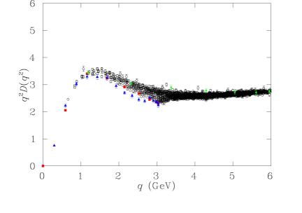
Figure 5: momentum-enhanced propagator from 76 configurations in $\partial^{2}\text{(III)}$ gauge from lattice 1w ($\beta=5.85,16^{3}\times 32$, Wilson action). There have been no data cuts. This is clearly a very bad gauge fixing.

IV.2 Coarser lattices

When comparing results from ensembles with different simulation parameters we need to consider three possible effects:

1. The dependence of $Z_{3}$ on the lattice spacing,

2. Errors due to the finite lattice spacing, especially when probing momenta near the cutoff,

3. Finite volume effects, especially in the infrared.

In Landau gauge, the dependence of the gluon propagator renormalization, $Z_{3}(a)$, on the cutoff is very weak. $Z_{3}$ is approximately constant with respect to the lattice spacing Bon01 . In this case it is easy to compare propagators produced on a wide range of lattice spacings. In Fig. 6 we plot the momentum-enhanced propagator on four lattices, which have $a=0.125$, 0.166, 0.270 and 0.353 fm. We see a very different situation to the one observed in Landau gauge Bon01 : the propagators appear to agree in the the deep infrared, yet diverge as the momentum increases. The difference is small for the two finest lattices - and non-existent in Fig. 1 - but quite dramatic for the coarsest.

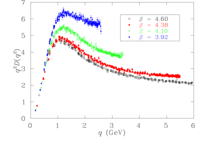
Figure 6: The momentum-enhanced propagator in $\partial^{2}\text{(II)}$ gauge at $\beta=4.60$, 4.38, 4.10 and 3.92 (ensembles 2i, 3, 4 & 5). Data has been cylinder cut. This figure shows the large sensitivity of $Z_{3}$ to lattice spacing in Laplacian gauge, quite unlike Landau gauge.

The correct way to compare the propagators is to normalize them at some common, “safe” momentum, i.e., one where we expect finite lattice spacing and finite volume effects to both be small. We choose $\mu=0.6$ GeV and show the results in Fig. 7. Multiplying the propagator by $q^{2}$ in constructing the momentum-enhanced propagator $q^{2}\,D(q^{2})$ reveals a rapid divergence in the ultraviolet. Yet normalizing at higher momenta results in data sets that agree nowhere except for at the scale $\mu$. It is interesting that the propagators from ensembles 5 and 6, which have the same lattice spacing, have slightly different normalizations.

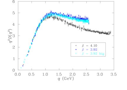
Figure 7: The momentum-enhanced propagator from ensembles 3, 4 and 5 in $\partial^{2}\text{(II)}$ gauge. Data has been cylinder cut and normalized at 0.6 GeV.

Also, as the lattice spacing is increased, the relative normalization between the gluon propagators in $\partial^{2}\text{(I)}$ and $\partial^{2}\text{(II)}$ gauges slowly diverges from one. As was seen above (Fig. 4), these two Laplacian gauges produce gluon propagators with rather different longitudinal components. The longitudinal part of the gluon propagator, multiplied by $q^{2}$, is plotted in $\partial^{2}\text{(I)}$ and $\partial^{2}\text{(II)}$ gauges for ensembles 4-6 in Fig. 8, using the same normalization determined for the transverse parts. Interestingly, the longitudinal part appears to be more affected by the finite volume of the lattice than the transverse part. In $\partial^{2}\text{(II)}$ gauge $q^{2}F(q^{2})$ may return to zero as $q^{2}\rightarrow 0$, while in $\partial^{2}\text{(I)}$ gauge a small, non-zero value appears likely, however, more work is required.

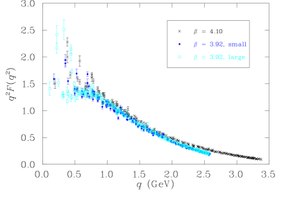
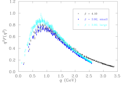
Figure 8: Comparison of the longitudinal part of the gluon propagator in $\partial^{2}\text{(I)}$ (top) and $\partial^{2}\text{(II)}$ (bottom) gauges for ensembles 4, 5 & 6. Data has been cylinder cut. The small and large $\beta=3.92$ lattices give diverging results even at large momenta in the $\partial^{2}\text{(II)}$ gauge.

In previous studies Ale01 ; Ale02 it was observed that the infrared gluon propagator saturates at a small volume ($\sim 1\text{ fm}^{4}$). To further explore this, we also study the propagator at zero four-momentum. As previously discussed, only the full propagator, $\mathcal{D}(0)$, can be calculated at zero four-momentum. In order to compare results on all of our lattices we normalize the data at 1 GeV. This represents a compromise and is certainly not ideal for all the data sets, hence there is some systematic error. These results are shown in Table 2.

	Dimensions	$\beta$	$a$ (fm)	Volume $\text{(fm}^{4}\text{)}$	$\mathcal{D}(0)$ - $\partial^{2}\text{(I)}$	$\mathcal{D}(0)$ - $\partial^{2}\text{(II)}$
1	$12^{3}\times 24$	4.60	0.125	10.1	16.6(5)	16.3(4)
2i	$16^{3}\times 32$	4.60	0.125	32.0	17.1(5)	16.0(4)
3	$16^{3}\times 32$	4.38	0.166	99.5	16.7(6)	14.1(3)
4	$12^{3}\times 24$	4.10	0.270	220	19.0(8)	14.6(2)
5	$10^{3}\times 20$	3.92	0.353	300	20.8(9)	14.6(4)
6	$16^{3}\times 32$	3.92	0.353	2040	52(5)	35(2)

Table 2: The full propagator at zero four-momentum in $\partial^{2}\text{(I)}$ and $\partial^{2}\text{(II)}$ gauges, normalized at 1 GeV for comparison.

If we restrict ourselves to ensembles 1-5, we see that, given the uncertainties discussed, the sensitivity of $\mathcal{D}(0)$ to volume is indeed small. We also see the trend, already noted above, for $\partial^{2}\text{(I)}$ and $\partial^{2}\text{(II)}$ gauges to become more different as the lattice spacing increases, another example of the discretization sensitivity of the Laplacian gauge. In the case of the very large lattice, ensemble 6, this sensitivity has become extreme.

We examine this another way through the transverse propagator, shown in Fig. 9 for ensembles 2i, 3 - 6. The data here corresponds to Table 2, having been normalized at 1 GeV. The propagators are consistent down to low momenta, $\sim 200$ MeV, where we strike trouble. Not only is there a spread between the data sets, but for ensemble 6, the point from purely temporal momentum is much lower than that from spatial momentum. The situation is the same in $\partial^{2}\text{(I)}$ gauge.

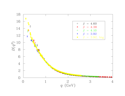
Figure 9: Comparison of the transverse part of the gluon propagator in $\partial^{2}\text{(II)}$ gauge for ensembles 1i, 2-6. Data has been cylinder cut. The propagators have been normalized at 1 GeV.

V Conclusions

We have made a detailed study of the gluon propagator on coarse lattices with an improved action in Laplacian gauges. We have described and tested three implementations of Laplacian gauge. $\partial^{2}\text{(I)}$ (QR decomposition) and $\partial^{2}\text{(II)}$ (Maximum trace) gauges produce similar results for the scalar transverse gluon propagator, but rather different longitudinal components. $\partial^{2}\text{(III)}$  for numerical reasons, works very poorly in $SU(3)$.

At sufficiently small lattice spacing, the transverse part of the gluon propagator is very similar in Laplacian gauge to that in Landau gauge. Laplacian gauge, however, exhibits great sensitivity to the lattice spacing, making results gained from coarse lattices difficult to compare with those from finer lattices. This is very different to the situation in Landau gauge. By comparing the coarse data sets at sufficiently low momentum, however, we have seen a great deal of consistency. In the deep infrared, the results from the largest lattice are difficult to reconcile with the other data. Excluding that lattice, the total propagator shows little sign of volume dependence. The most likely explanation of the (unimproved) Laplacian gauge results seen here is that on our coarsest lattices (improved lattices with $\beta=3.92$, 4.10, and to some extent even $\beta=4.38$), the lattice artifacts are much more severe than in the improved Landau gauge case. On the very coarse $\beta=3.92$ and 4.10 lattices, it seems very likely that finite volume and discretization errors are actually being coupled together by the Laplacian gauge fixing. By implementing an improved Laplacian gauge fixing on these lattices we anticipate that these errors will decouple on these lattices and we will be in a better position to estimate the infinite volume and continuum limits of the different implementations of Laplacian gauge-fixing. Further studies, including an improved Laplacian gauge fixing, will hopefully clarify these issues.

- (1) Jeffrey E. Mandula, The Gluon Propagator, hep-lat/9907020; L. von Smekal and R. Alkofer, What the Infrared Behavior of QCD Green Functions can tell us about Confinement in the Covariant Gauge, hep-ph/0009219; For a recent demonstration of the connection between the gluon propagator and confinement, see e.g., Kurt Langfeld, hep-lat/0204025.
- (2) D. Becirevic et al., Phys. Rev. D 60, 094509 (1999); D. Becirevic et al., Phys. Rev. D 61, 114508 (2000).
- (3) See, for example, C. D. Roberts and A. G. Williams, Prog. Part. Nucl. Phys. 33, 477 (1994).
- (4) A. Cucchieri and D. Zwanziger, Nucl. Phys. B (Proc. Suppl.) 106, 694 (2002).
- (5) L. Giusti et al., Nucl. Phys. B (Proc. Suppl.) 106, 995 (2002).
- (6) D.B. Leinweber, J-I. Skullerud and A.G. Williams, Phys. Rev. D 60, 094507 (1999); Erratum-ibid. D 61, 079901 (2000).
- (7) F.D.R. Bonnet, P.O. Bowman, D.B. Leinweber & A.G. Williams, Phys. Rev. D 62, 051501 (2000).
- (8) F.D.R. Bonnet, P.O. Bowman, D.B. Leinweber, A.G. Williams and J.M. Zanotti, Phys. Rev. D 64, 034501 (2001).
- (9) V.N. Gribov, Nucl. Phys. B 139, 1 (1978).
- (10) J.E. Hetrick & Ph. de Forcrand, Nucl. Phys. B (Proc. Suppl.) 63, 838 (1998).
- (11) J.F. Markham & T.D. Kieu, Nucl. Phys. B (Proc. Suppl.) 73, 868 (1999); O. Oliveira and P.J. Silva, Nucl. Phys. B (Proc. Suppl.) 106, 1088 (2002).
- (12) A.G. Williams, Nucl. Phys. B (Proc. Suppl.) 109, 141 (2002).
- (13) J.C. Vink and U-J. Wiese, Phys. Lett. B 289, 122 (1992).
- (14) J.C. Vink, Phys. Rev. D 51, 1292 (1995).
- (15) C. Alexandrou, Ph. de Forcrand and E. Follana, Phys. Rev. D 63, 094504 (2001).
- (16) C. Alexandrou, Ph. de Forcrand and E. Follana, hep-lat/0112043.
- (17) P.O. Bowman, U.M. Heller and A.G. Williams, hep-lat/0203001.
- (18) P. van Baal, Nucl. Phys. B (Proc. Suppl.) 42, 843 (1995).
- (19) J.E. Mandula, Nucl. Phys. B (Proc. Suppl.) 106, 998 (2002).
- (20) F.D.R. Bonnet, P.O. Bowman, D.B. Leinweber, A.G. Williams and J. Zhang, To appear in Physical Review, hep-lat/0202003.