UTCCP-P-122, UTHEP-456 Light Hadron Spectrum and Quark Masses from Quenched Lattice QCD

Abstract

We present details of simulations for the light hadron spectrum in quenched QCD carried out on the CP-PACS parallel computer. Simulations are made with the Wilson quark action and the plaquette gauge action on lattices of size $32^{3}\times 56-64^{3}\times 112$ at four values of lattice spacings in the range $a\approx 0.1$–0.05 fm and the spatial extent $L_{s}a\approx$ 3 fm. Hadronic observables are calculated at five quark masses corresponding to $m_{PS}/m_{V}\approx 0.75$–0.4, assuming the $u$ and $d$ quarks being degenerate but treating the $s$ quark separately. We find that the presence of quenched chiral singularities is supported from an analysis of the pseudoscalar meson data. Physical values of hadron masses are determined using $m_{\pi}$, $m_{\rho}$ and $m_{K}$ (or $m_{\phi}$) as input to fix the physical scale of lattice spacing and the $u$, $d$ and $s$ quark masses. After chiral and continuum extrapolations, the agreement of the calculated mass spectrum with experiment is at a 10% level. In comparison with the statistical accuracy of 1–3% and systematic errors of at most 1.7% we have achieved, this demonstrates a failure of the quenched approximation for the hadron spectrum: the hyperfine splitting in the meson sector is too small, and in the baryon sector the octet masses and the mass splitting of the decuplet are both smaller than experiment. Light quark masses are calculated using two definitions: the conventional one and the one based on the axial-vector Ward identity. The two results converge toward the continuum limit, yielding $m_{ud}=4.29(14)^{+0.51}_{-0.79}$ MeV where the first error is statistical and the second one is systematic due to chiral extrapolation. The $s$ quark mass depends on the strange hadron mass chosen for input: $m_{s}=113.8(2.3)^{+5.8}_{-2.9}$ MeV from $m_{K}$ and $m_{s}=142.3(5.8)^{+22.0}_{-0}$ MeV from $m_{\phi}$, indicating again a failure of the quenched approximation. We obtain the scale of QCD, $\Lambda_{\overline{\rm MS}}^{(0)}=$ 219.5(5.4) MeV with $m_{\rho}$ used as input. An $O(10\%)$ deviation from experiment is observed in the pseudoscalar meson decay constants.

I Introduction

Theoretical derivation of the light hadron spectrum from the first principles of Quantum Chromodynamics (QCD) is a fundamental issue in our understanding of the strong interactions. The binding of quarks due to gluons cannot be treated perturbatively, and numerical simulations based on the lattice formulation of QCD, therefore, provide a unique means to approach this problem.

The calculation of the hadron spectrum is made for given quark masses and hence it in turn enables us to determine the light quark masses, which are the fundamental parameters of QCD. The dynamical scale $\Lambda$ of QCD is determined by measurements of lattice spacing $a$ as a function of the bare coupling constant. Lattice QCD also provides us with a method to explore the chiral structure which is approximately realized in the real world. A further subsidiary verification of QCD may include the examination of the decay matrix elements against experiment.

Lattice QCD simulations, however, are computationally demanding, particularly when effects of dynamical quarks are to be included. Therefore, since the pioneering attempts in 1981 [1, 2], the majority of lattice QCD simulations have been made within the quenched approximation in which pair creation and annihilation of sea quarks are ignored. In fact such calculations have given hadron spectrum in a gross agreement with experiment, but clear understanding has not been achieved yet as to where this approximation would break down. In order to study this point, a calculation with a much higher precision is needed. Such a high precision study requires accurate controls of a number of systematic errors, which is not an easy task even within the quenched approximation. The origins of systematic errors include finiteness of lattice size, coarseness of lattice spacing and extrapolations in quark masses from relatively large values.

The work of GF11 Collaboration carried out in 1991–1993 [3] has advanced the control of systematic errors from a finite lattice spacing and a finite lattice size. Taking an advantage of large computing power, the GF11 Collaboration calculated the light hadron spectrum with three sets of the coupling constant and three different lattice sizes at one coupling constant, which is used to take continuum limit and estimate finite lattice effects. They claimed that the resulting spectrum is in agreement with experiment within 6%, the difference for each hadron being within their errors.

We feel that their results need a further verification by an independent analysis, since we consider that their conclusions depend crucially on the error estimate at simulation points, and on a rather long chiral extrapolation from the region of the pseudoscalar to vector meson mass ratio $m_{PS}/m_{V}=0.9$ – 0.5. Another issue is that GF11 simulations were made only for degenerate quarks. Masses of strange mesons and decuplet baryons were estimated using mass formulae, while strange octet baryons were not calculated.

We have embarked on the program to push the calculation of the quenched light hadron spectrum beyond that of the GF11 Collaboration to answer the posed problems. We have aimed to achieve a precision of a few percent for statistical errors and to reduce systematic errors to be comparable to or smaller than statistical errors. Taking the Wilson quark action and the plaquette gluon action, simulations are made with lattices of physical spatial size $L_{s}a\approx 3$ fm for the range of $a\approx 0.1$ – 0.05 fm. The smallest value of $m_{PS}/m_{V}$ is lowered to $\approx 0.4$. We take an advantage of the recent development of quenched chiral perturbation theory (Q$\chi$PT) [4, 5], which suggests us the form of chiral extrapolations. We assume that the light $u$ and $d$ quarks are degenerate, but the heavier $s$ quark is treated separately giving a different quark mass.

During the time, the MILC Collaboration carried out studies in a similar spirit [6] using the Kogut-Susskind quark action. Because of complications with the spin-flavor content of this action, they reported only the nucleon mass taking $m_{\pi}$ and $m_{\rho}$ as input, leaving aside all other hadrons.

Our calculation was made by the CP-PACS computer, a massively parallel computer developed at the University of Tsukuba completed in September 1996 [7]. With 2048 processing nodes, the peak speed of the CP-PACS is 614 GFLOPS (614 billion double precision floating-point operations per second). Our optimized program achieves a sustained speed of 237.5 GFLOPS for the heat-bath update of gluon variables and 264.6 GFLOPS for the over-relaxation update, and 325.3 GFLOPS for the quark propagator solver for which the core part is written in the assembly language [8]. The simulations were executed from the summer of 1996 to the fall of 1997.

A brief description of our results has been published in Ref. [9], and preliminary reports have appeared in Refs. [10]. In this article we present full details of analyses and results.

The organization of the paper is as follows: in Sec. II the lattice action and simulation parameters are explained. In Sec. III we present a summary of results for the light hadron spectrum, quark masses and meson decay constants. Subsequent sections describe details of our analyses. In Sec. IV measurements of hadron masses and quark masses at simulation points are discussed. We then examine in Sec. V the prediction of Q$\chi$PT for light hadron masses against our data. In Sec. VI we describe the extrapolation procedure of hadron masses to the chiral and continuum limits. Comparisons with other studies are given in this section. In Sec. VII we discuss determinations of the light quark masses, and in Sec. VIII, the QCD $\Lambda$ parameter. In Sec. IX results for meson decay constants are presented. Finally, Sec. X presents an alternative analysis in which the order of the chiral and continuum extrapolations are reversed. Our conclusions are given in Sec. XI. Technical details are relegated to Appendices A to G.

II Lattice action and simulation parameters

A Lattice action

We generate gauge configurations using the one-plaquette gluon action,

$$S_{g}=\frac{\beta}{3}\sum_{P}{\rm Re\,Tr}(U_{P}),$$ (1)

where $\beta=6/g^{2}$ with $g$ the bare gauge coupling constant. On gauge configurations, we evaluate quark propagators using the Wilson fermion action,

$$S_{q}=-\sum_{n,m}\bar{\psi}(n)D(\kappa;n,m)\psi(m),$$ (2)

$$D(\kappa;n,m)=\delta_{n,m}-\kappa\sum_{\mu}\{ (I-\gamma_{\mu})U_{n,\mu}\delta_{n+\hat{\mu},m}$$ (3)

$$+ (I+\gamma_{\mu})U^{\dagger}_{m,\mu}\delta_{m+\hat{\mu},n}\},$$ (4)

where the hopping parameter $\kappa$ controls the quark mass.

B Simulation parameters

Simulation parameters are summarized in Tables I and II. Four values of $\beta$ are chosen so as to cover the range of $a\approx 0.1$ – 0.05 fm ($a^{-1}\approx 2$–4 GeV).

We employ lattices with the physical extent of $L_{s}a\approx 3$ fm in the spatial directions. In a previous study, no significant finite lattice size effect was observed for $L_{s}a\geq 2$ fm beyond a statistical error of about 2% [11]. For a large lattice, the dominant size effect comes from spatial wrappings of pions whose magnitude decreases as $m_{L_{s}}-m_{\infty}\propto\exp(-c\,m_{\pi}L_{s})$[12]. For smaller lattices squeezing of hadron wave functions enhances the finite size effect, leading to a power low behavior, $m_{L_{s}}-m_{\infty}\propto c/L_{s}^{3}$[13, 14]. Assuming the latter behavior, we expect the finite-size effects on lattices with $L_{s}a\approx 3$ fm to be about 0.6%, which is sufficiently small compared with our statistical errors. This requires us to use a $64^{3}$ lattice for simulations at $a\approx$ 0.05 fm.

For the temporal extent of the lattices, we adopt $L_{t}=(7/4)\cdot L_{s}$. This gives the maximal physical time separation of $L_{t}a/2\approx 2.5$ fm. With our smearing method described below, we find that this temporal extent is sufficient to extract ground state signals in hadron propagators, suppressing contaminations from excited states.

For the quark mass, we select five values of $\kappa$, so that they give $m_{PS}/m_{V}\approx 0.75$, 0.7, 0.6, 0.5, and 0.4. The two heaviest values, which we denote as $s_{1}$ and $s_{2}$, are chosen to interpolate hadron mass data to the physical point of the $s$ quark. The three lighter quarks denoted as $u_{1}$, $u_{2}$ and $u_{3}$ are used to extrapolate to the physical point of the light $u$ and $d$ quarks, $m_{PS}/m_{V}=m_{\pi}/m_{\rho}=0.176$.

The quark mass at the smallest value of $m_{PS}/m_{V}\approx 0.4$ is closer to the chiral limit than that in any previous studies with the Wilson quark action, in which calculations were limited to $m_{PS}/m_{V}\hbox to0.0pt{\lower 3.5pt\hbox{$\mathchar 0\relax\sim$}\hss}\raise 1.0pt\hbox{$>$}0.5$. Reducing the quark mass further is not easy. Test runs we carried out for $m_{PS}/m_{V}\approx 0.3$ at $\beta=5.9$ show that fluctuations become too large and the computer time for this point alone exceeds the sum of those for the five $\kappa$ down to $m_{PS}/m_{V}\approx$ 0.4.

Gauge configurations are generated by the 5-hit pseudo-heat-bath algorithm[15] and an over-relaxation algorithm[16], mixed in the ratio of 1:4. We call the combination of one pseudo-heat-bath update sweep followed by four over-relaxation sweeps “iteration”. The periodic boundary conditions are imposed in all four directions. The acceptance rate in the pseudo-heat-bath step is 82–85% as listed in Table I. For vectorization and parallelization of the computer program, we adopt an even-odd algorithm.

After 2000–20000 thermalization iterations, we calculate quark propagators and measure hadronic observable on configurations separated by 200 to 2000 iterations depending on $\beta$, while we measure the gluonic observable, such as the plaquette expectation value, at every iteration. The total number of configurations and their separation are summarized in Table I.

We estimate errors by the jackknife method except otherwise stated. Tests on the bin size dependence do not show the presence of correlations between successive configurations, and hence we use the unit bin size for error analyses.

Table III shows the number of employed processors of the CP-PACS and the execution time required for generating and analyzing one configuration. Simulations at $\beta=$ 5.9, 6.1 and 6.25 are carried out on subpartitions of the CP-PACS computer while at $\beta=6.47$ the whole system with 2048 processing units is used.

III Summary of results

A Quenched chiral singularity

Quenched chiral perturbation theory (Q$\chi$PT) [4, 5] predicts that hadron mass as a function of quark mass $m_{q}$ exhibits a characteristic singularity in the chiral limit. Data for $m_{PS}^{2}$ strongly support the existence of an expected singular term $\delta m_{q}\ln m_{q}$ with $\delta\approx 0.1$. For vector mesons and baryons, the accuracy of mass data and the covered range of $m_{q}$ are not sufficient to establish the presence of quenched singularities.

In Figs. 1 to 4, the Q$\chi$PT fit is shown by solid lines for (a) pseudoscalar meson, (b) vector meson, (c) octet baryon and (d) decuplet baryon. The data are consistent with the theoretical expectations from Q$\chi$PT, not only for pseudoscalar mesons but also for vector mesons [17] and baryons [18]. We therefore adopt functional forms based on Q$\chi$PT for chiral extrapolations for all cases.

B Quenched light hadron spectrum

We take experimental values of $m_{\pi}=0.1350$ GeV and $m_{\rho}=0.7684$ GeV as input for the mean $u,d$ quark mass $m_{u,d}$ and the lattice spacing $a$. We use either $m_{K}=0.4977$ GeV or $m_{\phi}=1.0194$ GeV for the strange quark mass $m_{s}$. As shown by solid lines in Fig. 5, hadron masses determined at each $\beta$ are well described by a linear function of $a$.

The quenched hadron spectrum in the continuum limit is compared in Fig. 6 with experiment shown by horizontal bars, with the numerical values given in Table IV. Filled symbols use $m_{K}$ as input, and open ones employ $m_{\phi}$. The two error bars show both statistical error and the sum of statistical and systematic errors (see Sec. VI). Statistical errors are 1–2% for mesons and 2–3% for baryons. Estimated systematic errors are at worst 1.8$\sigma$ of statistical ones, which add only extra 1.7% to statistical ones.

Figure 6 shows that quenched QCD reproduces the global pattern of the light hadron spectrum reasonably well, but at the same time systematic deviations exist between the quenched spectrum and experiment. An important manifestation of this discrepancy is that the quenched prediction depends sizable on the choice of particle ($K$ or $\phi$) to fix $m_{s}$. While an overall agreement in the baryon sector is better if $m_{\phi}$ is employed as input, $m_{K}$ disagrees by 11% (6$\sigma$), which is the largest difference between our result and experiment.

In the meson sector, the discrepancy is seen in the hyperfine splitting, that is too small compared to experiment. If one uses the $m_{K}$ as input, the vector meson masses $m_{K^{*}}$ and $m_{\phi}$ are smaller by 4% (4$\sigma$) and 6% (5$\sigma$). If $m_{\phi}$ is employed instead, $m_{K^{*}}$ agrees with experiment within 0.8% (2$\sigma$) but $m_{K}$ is larger by 11% (6$\sigma$).

The smallness of the hyperfine splitting is observed in a different way in Fig. 7, which plots $m_{V}^{2}-m_{PS}^{2}$ as a function of $m_{PS}^{2}$. The figure shows an approximate scaling over the four values of $\beta$. The convergence of data toward the experimental point corresponding to ($m_{\pi}$,$m_{\rho}$) is due to our choice of these particles as input. Toward heavier quark masses, the mass square difference decreases faster than experiment, and is about 10% smaller at the point corresponding to $(m_{K},m_{K^{*}})$ mesons.

A faster decrease of $m_{V}^{2}-m_{PS}^{2}$ can be quantified through the $J$ parameter[19] defined by

$$J=m_{V}\frac{dm_{V}}{dm_{PS}^{2}}.$$ (5)

A large negative value of the slope seen in Fig. 7 translates into a small $J$ as shown in Fig. 8; we obtain

$$J=0.346(23)$$ (6)

in the continuum limit, to be compared with the experimental value $\sim 0.48$ at $m_{V}/m_{PS}=1.8$.

In the octet baryon sector, the masses are all smaller compared to experiment. The nucleon mass is lower than experiment by 7% ($2.5\sigma$). The strange octet baryons are lighter by 6–9% with $m_{K}$ as input, and by 2–5% even with $m_{\phi}$ as input. The $\Sigma$-$\Lambda$ hyperfine splitting is larger by 30% (50%) with $m_{K}$ ($m_{\phi}$) input, though the deviation of $0.8\sigma$ ($2.3\sigma$) is statistically marginal. The Gell-Mann-Okubo (GMO) relation

$$\frac{1}{2}(m_{N}+m_{\Xi})=\frac{1}{4}(3m_{\Lambda}+m_{\Sigma})$$ (7)

based on first-order flavor $SU(3)$ breaking is well satisfied, at 1% in both $m_{K}$ and $m_{\phi}$ input, though the two sides take values (1.04(2) GeV for the $m_{K}$-input and 1.09(1) GeV for the $m_{\phi}$-input) smaller than experiment (1.13 GeV).

For decuplet baryons, the mass of $\Delta$ turns out to be consistent with experiment within statistical error of 2.0% (0.7$\sigma$). An equal spacing rule is well satisfied, the three spacings mutually agreeing within statistical errors. However, the mass splitting is smaller by 30% on average compared to experiment for $m_{K}$ input, and by 10% for $m_{\phi}$ input.

The results discussed above are based on Q$\chi$PT chiral fits. In order to see effects of choosing different chiral fit functions, we repeat the procedure using low-order polynomials in $m_{q}$, as was done in traditional analyses. Chiral fits and continuum extrapolations for this case are illustrated in Figs. 1 to 4 by dashed lines and in Fig. 5 by open symbols and dashed lines, respectively. Q$\chi$PT and polynomial fits lead to masses which agree within 1.5% or $1.6\sigma$. The pattern of the quenched spectrum remains the same even if one adopts the polynomial chiral fits.

C Reversibility of order of the chiral and continuum extrapolations

In order to obtain the physical hadron mass, one conventionally carries out chiral extrapolation first and then takes the continuum extrapolation (we refer to this as method A). These two limiting operations can in principle be reversed, and the resulting spectrum should be unchanged. An advantage with the reversed limiting procedure (method B) is that one need not worry about possible $O(a)$ terms that are present in Q$\chi$PT formulae at finite lattice spacings.

The light hadron spectrum from the two methods are compared in Fig. 9 for the case of the $m_{K}$ input. The prediction from the method B denoted by open symbols is in good agreement with that of the method A plotted with filled symbols within $1.5\sigma$.

An additional advantage of method B is that the hadron mass formula can be obtained as a function of an arbitrary quark mass, as shown in the Edinburgh plot in Fig. 10.

D Fundamental parameters of QCD

The scale parameter $\Lambda$ is the fundamental parameter of QCD. We evaluate it in the $\overline{\rm MS}$ scheme to be

$$\Lambda_{\overline{\rm MS}}^{(0)}=219.5(5.4){\rm\ MeV},$$ (8)

when the scale is fixed by $m_{\rho}$.

The definition of quark mass for the Wilson quark action is not unique, because chiral symmetry is broken by terms of $O(a)$. We analyze quark masses from two definitions, the conventional one through the hopping parameter, which we call the VWI quark mass (see Sec.  IV C), and another defined in terms of the Ward identity for axial-vector currents (AWI).

Figures 11 and 12 show $m_{ud}$ and $m_{s}$ renormalized in the $\overline{\rm MS}$ scheme at $\mu=2$ GeV as functions of $a$. The VWI and AWI quark masses, differing at finite $a$, extrapolate to a universal value in the continuum limit, in accordance with a theoretical expectation.

A combined linear extrapolation assuming a unique value in the continuum limit yields

$$m_{ud} = 4.29(14)^{+0.51}_{-0.79}\;\;{\rm MeV}$$ (9)

$$m_{s} = 113.8(2.3)^{+5.8}_{-2.9}\;\;{\rm MeV}\ \ \ m_{K}{\rm-input},$$ (10)

$$= 142.3(5.8)^{+22.0}_{-0}\;\;{\rm MeV}\ \ \ m_{\phi}{\rm-input}.$$ (11)

We indicate systematic error arising mainly from chiral extrapolations. The value of $m_{s}$ differs by about 20% depending on $m_{K}$ or $m_{\phi}$ used as input. The difference arises from the small value of meson hyperfine splitting in the simulation.

E Meson decay constants

The pseudoscalar meson decay constant $f_{PS}$ is defined by

$$\langle 0|A_{\mu}|{\rm PS}\rangle=ip_{\mu}f_{PS},$$ (12)

in the continuum notation, where $A_{\mu}$ is the axial-vector current. The experimental value for $\pi$ is $f_{\pi}=132$ MeV. Data for $f_{PS}$ are shown in Fig. 13 as a function of $a$. We obtain for physical values

$$f_{\pi} = 120.0(5.7)\text{\ MeV},$$ (13)

$$f_{K} = 138.8(4.4)\text{\ MeV}\ \ \ m_{K}{\rm-input}.$$ (14)

These values are smaller than experiment by 9% (2$\sigma$) and 13% (5$\sigma$), respectively. Q$\chi$PT predicts that the ratio $f_{K}/f_{\pi}-1$ in the quenched QCD is smaller than experiment by about 30%. This quantity is shown in Fig. 14. We obtain $f_{K}/f_{\pi}-1=0.156(29)$ which is smaller than experiment by 26% ($1.9\sigma$) as Q$\chi$PT predicts.

The vector meson decay constant $F_{V}$ in the continuum theory is defined by

$$\langle 0|V_{i}|V\rangle=\epsilon_{i}F_{V}m_{V},$$ (15)

where $\epsilon_{i}$ and $m_{V}$ are the polarization vector and the mass of the vector meson $V$. This is related with another conventional definition by $f^{-1}_{V}=F_{V}/m_{V}$. The experimental value of $F_{\rho}$ is 220(5) MeV, where the charge factor is removed. Figure 15 summarizes the vector meson decay constants. We obtain

$$F_{\rho} = 205.7(6.6)\text{\ MeV},$$ (16)

$$F_{\phi} = 229.4(5.7)\text{\ MeV}\ \ \ m_{\phi}{\rm-input}.$$ (17)

These values are slightly smaller than experiment; by 6.7% (2.2$\sigma$) for $F_{\rho}$ and by 3.8% (1.6$\sigma$) for $F_{\phi}$.

We summarize meson decay constants in Table V.

IV Measurements of hadron masses and quark masses

A Quark propagators

We calculate the quark propagator $G(m)$ at a value of $\kappa$ by solving

$$\sum_{m}D(\kappa,n,m)G(m)=S(n),$$ (18)

where $D(\kappa,n,m)$ is the quark matrix defined in Eq. (4), and $S(n)$ is the quark source. In order to enhance the ground state signal in the hadronic measurements, we use smeared quark sources. For this purpose, we fix gauge configurations to the Coulomb gauge as described in Appendix A.

For the smeared source, we employ an exponential form given by

$$S(n)=\left\{\begin{array}[]{ll}A\exp(-B|n|)&\quad\mbox{for}\quad n\neq 0\\ 1.0&\quad\mbox{for}\quad n=0\end{array}\right.,$$ (19)

as motivated by the pion wave function measured by the JLQCD Collaboration[21]. The smearing radius is approximately constant, $a/B\approx 0.33$ fm, over the range of $\beta$ we simulate. The quark propagator solver and the smearing function are discussed in Appendix B.

B Hadron masses

From quark propagators, we construct hadron propagators corresponding to degenerate combinations, $ff$ and $fff$ ($f=s_{1},s_{2},u_{1},u_{2},u_{3}$), as well as non-degenerate combinations of the type $s_{i}u_{j}$ for mesons, and $s_{i}s_{i}u_{j}$ and $s_{i}u_{j}u_{j}$ for baryons; two quarks in baryons are taken to be degenerate. We study pseudoscalar and vector mesons, and spin $1/2$ octet and spin $3/2$ decuplet baryons. The hadron operators are summarized in Appendix C.

Hadron propagators are calculated for all possible combinations of point and smeared sources. At the sink we use only point operators. Effective masses $m_{eff}(t)$ for various combination of quark sources are compared in Fig. 16. With our choice of smearing function, $m_{eff}(t)$, in almost all cases reaches a plateau from above, suggesting that the smearing radius is smaller than the actual spread of hadron wave functions. The onset of plateau is the earliest when the smeared source is used for all quarks, and statistical error is the smallest for this case. In light of this advantage, we extract masses from hadron propagators with all quark sources smeared.

In order to illustrate the quality of data, typical effective masses are shown in Figs. 17–20 for degenerate octet baryons at the four $\beta$ values. We extract the ground state masses using a single hyperbolic cosine fit for mesons and a single exponential fit for baryons, taking account of correlations among different time slices. In Figs. 17–20, the horizontal lines are the fit and error, with the range of the lines representing the fit range.

The fit range $[t_{min},t_{max}]$ is chosen based on the following observations: (1) Value of $\chi^{2}/N_{df}$ decreases as $t_{min}$ increases and becomes almost constant at a time slice which we denote as $t_{\chi}$. $t_{\chi}$ in general depends on quark masses. (2) The effective mass shows a plateau for $t\hbox to0.0pt{\lower 3.5pt\hbox{$\mathchar 0\relax\sim$}\hss}\raise 1.0pt\hbox{$>$}t_{\chi}$. (3) When $t_{max}\geq t_{\chi}+3$, $\chi^{2}/N_{df}$ is insensitive to the choice of $t_{max}$. From these findings, we may use $t_{\chi}$ for $t_{min}$. However, in order to avoid subjectivity in the identification of $t_{\chi}$ and plateau, we adopt $t_{min}$ which satisfies the following conditions:

• $t_{min}$ is larger than $t_{\chi}$.

• For each kind of particle at each $\beta$, $t_{min}$ is common to all quark masses.

• For each particle, values of $t_{min}$ in physical units is approximately constant for all $\beta$.

We find that these conditions are satisfied by $t_{min}\approx 1.0$ fm, 0.7 fm and 0.5 fm for pseudoscalar mesons, vector mesons and baryons, respectively.

The largest time slices $t_{max}$ for vector mesons and baryons at $\beta=5.9$, 6.1 and 6.25 are chosen by the requirement that the error of propagator at $t_{max}$ does not exceed 3%. We employ the same criterion for vector mesons at $\beta=6.47$. For baryons at $\beta=6.47$, the fitting interval becomes too narrow for light quark masses if we employ the cut at 3%. We therefore adopt the cuts at 3.2% for octet baryons and 4% for decuplet baryons, respectively.

Values of $t_{max}$ are determined with a different strategy for pseudoscalar mesons, for which we make chiral extrapolations taking account of correlations among different quark masses. (Correlation among different quark masses is ignored for other hadrons.) A large value of $t_{max}$ results in full covariance matrices with too large dimensions. Such matrices frequently have quite small eigenvalues due to statistical fluctuations, and lead to a failure of the convergence of the fit. In order to avoid instability of chiral extrapolations, we determine $t_{max}$ by trial and error. We adopt $t_{max}=28$, 35, 25 and 35 for $\beta=5.9$, 6.1, 6.25 and 6.47.

All hadron masses are stable under a variation of the fit range. As an example, the fits with the range $[t_{min}+2,t_{max}]$ give results consistent within $1\sigma$. Uncorrelated fits yield masses consistent with those from correlated fits within 1$\sigma$ for most cases, although the differences are about 2$\sigma$ for some cases.

Errors are determined by a unit increase of $\chi^{2}$. Jackknife errors are similar in magnitude, the difference being at most about 25%. The values of $\chi^{2}/N_{df}$ turn out to be consistent or smaller than unity within errors estimated by the jackknife method, meaning that our one-mass fits reproduce the hadron propagator data well. This suggests that the contamination of excited states are well suppressed in our fits. Our results for the hadron masses are reproduced in Tables VI for mesons and Tables VII and VIII for octet and decuplet baryons.

C Quark masses

The bare quark mass is conventionally defined by

$$m_{q}^{VWI(0)}=\frac{1}{2}\left(\frac{1}{\kappa}-\frac{1}{\kappa_{c}}\right),$$ (20)

where $\kappa_{c}$ is the critical hopping parameter at which the pion mass vanishes. This quark mass is called the vector Ward identity(VWI) quark mass, since the divergence of the vector current is proportional to the mass difference of quark flavors in the current, which looks similar to Eq. (20).

The definition of the AWI quark mass is based on the Ward identity for axial-vector currents [22]. For the flavor combination $(f,g)$, it takes the form,

$$\frac{1}{a}\langle\overline{\nabla}_{\mu}A_{\mu}(n){\cal O}\rangle = (m_{f}+m_{g})\langle P(n){\cal O}\rangle$$ (22)

$$+\langle\delta{\cal O}\rangle+O(a),$$

where

$$A_{\mu}(n)=\frac{1}{2}\Big{\{}\bar{f}_{n+\hat{\mu}}U_{n,\mu}^{\dagger}i\gamma_{\mu}\gamma_{5}g_{n}+\bar{f}_{n}U_{n,\mu}i\gamma_{\mu}\gamma_{5}g_{n+\hat{\mu}}\Big{\}}$$ (23)

is the axial-vector current and

$$P(n)=\overline{f}_{n}\gamma_{5}g_{n}$$ (24)

is the pseudoscalar density. In Eq.(22), $\overline{\nabla}_{\mu}F(n)=F(n)-F(n-\hat{\mu})$ is the backward lattice derivative, and $\delta{\cal O}$ is the response of the operator ${\cal O}$ under the chiral transformation. The $O(a)$ term is due to explicit violation of chiral symmetry with the Wilson quark action.

In order to extract $m_{q}^{AWI(0)}$, we use the relation [23]

$$m_{f}^{AWI(0)}+m_{g}^{AWI(0)}=\lim_{t\to\infty}\frac{\langle\overline{\nabla}_{4}A_{4}(t)P(0)\rangle}{\langle P(t)P(0)\rangle},$$ (25)

where

$$A_{4}(t)= \sum_{\vec{n}}A_{4}(n=({\vec{n}},t)),$$ (26)

$$P(t)= \sum_{\vec{n}}P(n=({\vec{n}},t)).$$ (27)

are projected to zero spatial momentum. The right-hand side of Eq.(25) is evaluated by a constant fit to the ratio

$$\frac{\langle\overline{\nabla}_{4}A_{4}(t)P(0)\rangle_{\rm sym}}{\langle P(t)P(0)\rangle},$$ (28)

where the suffix $sym$ implies a symmetrization of the derivative defined by

$$\langle\overline{\nabla}_{4}A_{4}(t)P(0)\rangle_{\rm sym}\equiv$$ (29)

$$(G(t)-G(t-1)+G(L_{t}-t)-G(L_{t}-t-1))/4$$ (30)

with $G(t)=\langle A_{4}(t)P(0)\rangle$. For the pseudoscalar operator at the origin, we use the smeared source for two quarks. Figures 21 and 22 illustrate our data for Eq. (28) at $\beta=5.9$ and 6.47. The constant fit is carried out without taking account of correlations between different time slices or between the two correlators. Fit ranges are determined from the plateau of the effective mass. The results for $m_{f}^{AWI(0)}+m_{g}^{AWI(0)}$ are summarized in Table IX.

V Quenched chiral singularities

The chiral extrapolation is conventionally carried out assuming a low-order polynomial in quark masses. Chiral perturbation theory[24], however, predicts a singular quark mass dependence in the chiral limit due to the presence of massless pions. The singularity is expected to be enhanced in quenched QCD [4, 5] since the $\eta\prime$ meson is also massless in this approximation. In order to choose the functional form for the chiral extrapolation, we examine whether hadron mass data are consistent with the predictions of Q$\chi$PT.

A Mass ratio test for pseudoscalar meson

For pseudoscalar mesons made of quarks with masses $m_{1}$ and $m_{2}$, Q$\chi$PT predicts the mass formula[4, 5] given by

$$m_{PS,12}^{2}=$$ (31)

$$A\,(m_{1}+m_{2})\Big{\{}1-\delta\big{[}\ln\frac{2m_{1}A}{\Lambda_{\chi}^{2}}+\frac{m_{2}}{m_{2}-m_{1}}\ln\frac{m_{2}}{m_{1}}\big{]}$$ (32)

$$+\frac{\alpha_{\Phi}A}{12\pi^{2}f^{2}}\big{[}m_{1}\ln\frac{2m_{1}A}{\Lambda_{\chi}^{2}}+m_{2}\ln\frac{2m_{2}A}{\Lambda_{\chi}^{2}}$$ (33)

$$+\frac{m_{1}m_{2}}{m_{2}-m_{1}}\ln\frac{m_{2}}{m_{1}}\big{]}\Big{\}}$$ (34)

$$+B\,(m_{1}+m_{2})^{2}+O(m^{3},\delta^{2}),$$ (35)

where terms proportional to $(m_{1}-m_{2})^{2}$ are absent[25]. The logarithmic term proportional to $\delta$ represents the leading quenched singularity. To the leading order in the $1/N_{c}$ expansion in terms of the number of colors $N_{c}$, $\delta$ is related to the pseudoscalar meson mass and the pion decay constant $f$ by

$$\delta=\frac{m_{\eta^{\prime}}^{2}+m_{\eta}^{2}-2m_{K}^{2}}{24\pi^{2}f^{2}}.$$ (36)

Taking the experimental values of $f$ and pseudoscalar meson masses, one finds $\delta\approx 0.2$ as a phenomenological estimate. The constant $\alpha_{\Phi}$ in Eq.(35) represents the coefficient of the kinetic term of the flavor singlet meson field, which is sub-leading in terms of $1/N_{c}$. The mass formula also contains a scale $\Lambda_{\chi}$ of $O(1)$ GeV. The parameters such as $\delta,\alpha_{\Phi}$ and $\Lambda_{\chi}$ may differ in quenched QCD from those in the full theory.

In order to see whether pseudoscalar mass data exhibit the presence of the logarithmic terms, we investigate the ratio $m_{PS,12}^{2}/(m_{1}+m_{2})$ as a function of $m_{1}+m_{2}$. We use the AWI quark mass rather than the VWI mass to avoid uncertainties due to the necessity of choosing $\kappa_{c}$, which in turn depends on details of chiral extrapolations. Another important point with the use of the AWI quark mass is that it is free from chiral singularities which cancel between the numerator and the denominator in Eq. (25) [25, 26].

In Fig. 23, we plot $m_{PS,12}^{2}/(m_{1}+m_{2})$ as a function of $m_{1}+m_{2}$. The AWI quark mass is converted to renormalized values in the ${\overline{\rm MS}}$ scheme at the scale 2 GeV (see Sec. VII) and the ratio is translated to physical units. This enables us to compare the results at different values of $\beta$ with the same scale of the figure. We find a clear increase of the ratio towards the chiral limit at all values of $\beta$ as expected from Eq. (35).

In order to make a more quantitative analysis, we consider the ratio defined by

$$y={\frac{2m_{1}}{m_{1}+m_{2}}\frac{m_{PS,12}^{2}}{m_{PS,11}^{2}}}\times{\frac{2m_{2}}{m_{1}+m_{2}}\frac{m_{PS,12}^{2}}{m_{PS,22}^{2}}}.$$ (37)

Assuming that $\delta$ and $\alpha_{\Phi}$ as well as quark masses are small, we expect

$$y=1+\delta\,x+\alpha_{X}\,z+O(m^{2},\delta^{2}),$$ (38)

where

$$\alpha_{X}=\frac{\alpha_{\Phi}A^{2}}{12\pi^{2}f^{2}},$$ (39)

and the parameters

$$x=2+\frac{m_{1}+m_{2}}{m_{1}-m_{2}}\ln\Big{(}\frac{m_{2}}{m_{1}}\Big{)},$$ (40)

and

$$z=\frac{1}{A}\Big{(}\frac{2m_{1}m_{2}}{m_{2}-m_{1}}\ln\frac{m_{2}}{m_{1}}-m_{1}-m_{2}\Big{)},$$ (41)

represent terms of $O(m_{q}\ln m_{q})$ and $O(m_{q}^{2}\ln m_{q})$ in Eq. (35).

We plot $y$ as a function of $x$ in Fig. 24, with numerical values listed in Table X. The points fall within a narrow ridge limited by two lines $y\approx 1+(0.08$–$0.12)\,x$. A one-parameter fit ignoring $\alpha_{X}z$ and higher order terms yields $\delta=0.10$–0.12 depending on $\beta$ as listed in Table XI.

A two-parameter fit keeping the $\alpha_{X}z$ term requires the value of $A$. We estimate $A\approx$ 3 GeV for all $\beta$ values from data at $m_{PS}/m_{V}$=0.75 and 0.7, assuming $m_{PS}^{2}=2Am_{q}$. Setting $f=132$ MeV, we obtain $\delta$ and $\alpha_{\Phi}$ given in the right column of Table XI. For the two finer lattices at $\beta=6.25$ and 6.47, $\alpha_{\Phi}$ is consistent with zero and $\delta\approx 0.1$. At the coarser lattices the values of $\alpha_{\Phi}$ and $\delta$ are not stable.

Further data are needed to pin down precise values of $\delta$ and $\alpha_{\Phi}$. We consider results at finer lattices, closer to the continuum limit, are more reliable, and take $\delta=0.10(2)$ and $\alpha_{\Phi}=0$ as our best estimate.

The ratio test for the existence of quenched logarithm terms was originally proposed in Ref. [5], in which one plots $y_{0}$ defined by

$$y_{0}=\frac{m_{PS,12}^{2}}{m_{PS,11}^{2}}\frac{2m_{1}}{m_{1}+m_{2}}$$ (42)

as a function of $x_{0}$ defined by

$$x_{0}=1+\frac{m_{2}}{m_{1}-m_{2}}\ln\Big{(}\frac{m_{2}}{m_{1}}\Big{)}.$$ (43)

The relation $y_{0}=1+\delta\cdot x_{0}$ follows if we ignore $O(m_{q}^{2})$ term in Eq.(35). As shown in Fig. 25, however, $y_{0}$ systematically varies with quark masses, suggesting a contribution from the $O(m_{q}^{2})$ term. The double ratio defined by Eq. (37) is designed to cancel the $O(m_{q}^{2})$ terms, and hence is more effective to observe the quenched singularity.

B Ratio test of pseudoscalar meson decay constant

Quenched chiral singularities are also expected in meson decay constants [27]. Let $f_{fg}$ be the pseudoscalar meson decay constant for the flavor combination $(f,g)$. In Ref. [27], the ratio

$$y_{f}=\frac{f_{12}^{2}}{f_{11}f_{22}}$$ (44)

was shown to satisfy the relation

$$y_{f}=1-\frac{\delta}{2}\,x$$ (45)

with $x$ defined by Eq.(40), where $\alpha_{\Phi}$ is set to zero. Values of $y_{f}$ are listed in Table X and the ratio test with Eq.(44) is summarized in Fig. 26. We find $\delta\approx 0.08$–0.16, in agreement with the value from the mass ratio analysis.

C Pseudoscalar meson mass fit

The parameter $\delta$ is estimated also by fitting pseudoscalar meson mass data to Eq. (35) assuming $\alpha_{\Phi}=0$ for all $\beta$. The AWI quark mass introduces errors in the fit variable. Therefore the VWI quark mass, $m_{q}^{VWI(0)}=(1/\kappa-1/\kappa_{c})/2$, is employed taking $\kappa_{c}$ as a parameter. We carry out fully-correlated fits described in Appendix D, independently for degenerate and non-degenerate cases.

A noticeable property of the Q$\chi$PT formula Eq. (35) is that $A$, $\delta$ and $\Lambda_{\chi}$ cannot be determined simultaneously because the three conditions to minimize $\chi^{2}$ are not mathematically independent. A possible method is to fix $f_{\Lambda}\equiv 2A^{2}/\Lambda_{\chi}^{2}$. Values of $A$ and $\delta$ depend on the choice of $f_{\Lambda}$, while $\kappa_{c}$ and $B$, as well as $\chi^{2}$ and the fit curve are independent. We consider $f_{\Lambda}=$ 4, 8, 16, and 32, which correspond to $\Lambda_{\chi}\approx 1.32$, 1.00, 0.76, and 0.57 GeV, respectively. This range of $\Lambda_{\chi}$ contains a natural scale for chiral perturbation theory, $\Lambda_{\chi}=m_{\rho}$, or 1 GeV.

The results are summarized in Table XIII. The value of $\delta$ is stable against a variation of $f_{\Lambda}$ and $\beta$, and is consistent within $2\sigma$ with our estimate 0.10(2) from the mass ratio test.

D Comparison with other results for $\delta$

The value of $\delta$ has recently been estimated by other groups. The FNAL group reported $\delta=0.065(13)$ [28] using the clover quark action, and the QCDSF Collaboration obtained $\delta\approx 0.14(2)$ [29] with a non-perturbatively improved clover action. These estimates are consistent with ours.

It has been pointed out in Ref. [30] that the $x$–$y$ correlation seen in Fig. 24 may be reproduced with a small $\delta\approx$ 0.03 – 0.07, if $\alpha_{\Phi}\approx$ 0.5. Our data for large $\beta$, however, do not seem to be compatible with such a large $\alpha_{\Phi}$.

E Vector meson and baryon masses

Q$\chi$PT predicts singularities of the form $O(m_{PS})\sim O(\sqrt{m_{q}})$ for vector mesons and baryons [17, 18]. The ratio tests similar to those for the pseudoscalar mesons indicate that the coefficient of the $O(m_{PS})$ term is non-vanishing both for vector mesons and baryons. It is difficult, however, to reliably estimate the coefficients from the ratios because of large errors. Direct fits of mass data to Q$\chi$PT formula are also difficult as they are not very stable. While our data are consistent with Q$\chi$PT, statistics and the range of the quark mass in our study do not allow conclusive results. Our tests of the Q$\chi$PT mass formulae for these cases are described in Appendix F.

VI Hadron mass spectrum

A Chiral fits

Chiral fits of the pseudoscalar meson mass are already described in Sec. V C, and are shown in Figs. 1-(a) –  4-(a) with parameters summarized in Table XII. Comparisons of various fit functions for pseudoscalar meson masses are given in Appendix E.

For vector mesons and baryons, we choose the pseudoscalar meson mass as the variable to represent the quark mass dependence. For vector mesons we adopt[17]

$$m_{V,12} = m_{V}^{0}$$ (48)

$$+\frac{C_{1/2}}{6}\{\frac{3}{2}(m_{11}+m_{22})+2\frac{m_{22}^{3}-m_{11}^{3}}{m_{22}^{2}-m_{11}^{2}}\}$$

$$+\frac{C_{1}}{2}(m_{11}^{2}+m_{22}^{2}),$$

where $m_{fg}$ is the pseudoscalar meson mass with the quark flavor combination $(f,g)$. The coefficient $C_{1/2}$ is proportional to $\delta$ while the $C_{1}$ term is present in ordinary $\chi$PT. For octet baryons, we employ[18]

$$m_{\Sigma} = m_{O}^{0}$$ (53)

$$+\frac{1}{2}\{4F^{2}w_{uu}-4(D-F)Fw_{ud}+(D-F)^{2}w_{ss}\}$$

$$-4b_{F}m_{uu}^{2}+2(b_{D}-b_{F})m_{ss}^{2}$$

$$+(2D^{2}/3-2F^{2})v_{uu}$$

$$+(2D^{2}/3-4DF+2F^{2})v_{ud},$$

$$m_{\Lambda} = m_{O}^{0}$$ (59)

$$+\frac{1}{2}\{(4D/3-2F)^{2}w_{uu}+(D/3+F)^{2}w_{ss}$$

$$-2(4D/3-2F)(D/3+F)w_{ud}\}$$

$$+4(2b_{D}/3-b_{F})m_{uu}^{2}-2(b_{D}/3+b_{F})m_{ss}^{2}$$

$$+(2D^{2}/9-8DF/3+2F^{2})v_{uu}$$

$$+(10D^{2}/9-4DF/3-2F^{2})v_{ud},$$

for $\Sigma$-type and $\Lambda$-type cases. For decuplet, the formula reads,

$$m_{D} = m_{D}^{0}+\frac{5H^{2}}{162}(4w_{uu}+4w_{ud}+w_{ss})$$ (62)

$$+\frac{C^{2}}{18}(w_{uu}-2w_{ud}+w_{ss})$$

$$+c(2m_{uu}^{2}+m_{ss}^{2}).$$

Here

$$w_{fg} = -2\pi\delta\frac{m_{ff}^{3}-m_{gg}^{3}}{m_{ff}^{2}-m_{gg}^{2}}$$ (63)

$$v_{fg} = \frac{m_{fg}^{3}}{8\pi f^{2}}.$$ (64)

The $O(m_{PS}^{3})$ terms are not included in Eq. (48) for vector mesons and in Eq. (62) for decuplet baryons. The octet-decuplet coupling terms are also ignored in Eqs.(53) and (59) for octet baryons. These choices are made because fitting parameters are not well determined if these terms are introduced (see Appendix F), and the dropped terms have small effects for the spectrum. Fittings with and without them are compared in Fig.27 for degenerate masses at $\beta=5.90$. The two types of fittings reproduce data equally well. The difference remains small at the physical point, at most 5% ($5\sigma$) at finite lattice spacings and at most 1.2% ($1.3\sigma$) after the continuum extrapolation.

We set $\delta=0.1$ and $\alpha_{\Phi}=0$ as suggested from the pseudoscalar case. These choices do not affect the fits for vector mesons and decuplet baryons: a non-vanishing $\alpha_{\Phi}$ leads to $O(m_{fg}^{3})$ effect which is not included in the fit function, and a change of $\delta$ is absorbed by a redefinitions of the parameters.

For the nucleon mass, dropping $O(m_{PS}^{3})$ terms in Eq. (53) would lead to a positive curvature (concave function), which contradicts the data that show a negative curvature (convex function) in Figs. 1-(c) – 4-(c). Therefore we include $O(m_{PS}^{3})$ terms for octet baryons. The coefficient of $O(m_{PS}^{3})$ terms is affected by the choice of $\delta$ and $\alpha_{\Phi}$. We study the effect of the uncertainty of $\delta$ and $\alpha_{\Phi}$ on the resulting octet masses by varying $\delta$ from 0.08 to 0.12 and $\alpha_{\Phi}$ from $-0.7$ to $+0.7$. The change of $\delta$ in this range results in $0.4$% (1.3$\sigma$) difference at finite lattice spacings and 0.3% (0.3$\sigma$) in the continuum limit. The change of $\alpha_{\Phi}$ leads to differences of 2.9%(4.7$\sigma$) and 2.2%(1.4$\sigma$), respectively. We also fix $f=f_{\pi}=$ 132 MeV. Changing $f$ to $f_{K}=226$ MeV affects octet baryon masses by at most 2.5$\sigma$ at finite lattice spacings, and 0.5$\sigma$ in the continuum limit. Artifacts of fixing these parameters are sufficiently small at least in the continuum limit.

Fits are made to degenerate and non-degenerate data together. Because the size of covariance matrix becomes too large and the matrix elements cannot be determined reliably, we do not include correlations among different quark masses.

Fits for vector mesons and baryons are shown in Figs. 1 to 4. Parameters are summarized in Table XIV for vector mesons, in Table XV for octet baryons and in Table XVI for decuplet baryons. As we see in the figures and tables, Q$\chi$PT fits reproduce data at all $\beta$.

B Hadron masses at the physical point

The extrapolation and interpolation to the physical point is made as follows. For the case of the $m_{K}$-input, we determine $m_{PS}(\kappa_{ud},s_{1})$ and $m_{PS}(\kappa_{ud},s_{2})$ from non-degenerate fits to pseudoscalar mesons, and interpolate them linearly in terms of the $s$ quark mass so that $m_{PS}(\kappa_{ud},\kappa_{s})$ takes the experimental value of $m_{K}$. For the $m_{\phi}$-input, we first determine the mass $m_{ss}$ of the degenerate pseudoscalar meson consisting of two strange quarks from the vector meson mass fit and evaluate $\kappa_{s}$. We then make a linear interpolation of $m_{PS}(\kappa_{ud},s_{1})$ and $m_{PS}(\kappa_{ud},s_{2})$ to find $m_{K}=m_{PS}(\kappa_{ud},\kappa_{s})\equiv m_{us}$. Values of $m_{uu}$, $m_{ss}$ and $m_{us}$ then lead to the predictions for other hadron masses.

Hadron masses in lattice units are listed in Table XVII. We include results for fictitious hadrons such as “$\eta_{s}=\bar{s}s$” (pseudoscalar meson consisting of two strange quarks), $\Lambda_{ss}$ ($\Lambda$-like baryon consisting of two quarks with $m_{s}$ and a light quark with $m_{ud}$), and $N_{sss}$ (octet baryon consisting of three quarks with $m_{s}$). Hadron masses translated to physical units are compiled in Table XVIII.

C Continuum extrapolation

For our lattice actions scaling violation is given by

$$m(a)=m(0)[1+Sa+(S^{\prime}a)^{2}+O(a^{3})].$$ (65)

Hadron mass data in Fig. 5 are fitted well without the $O(a^{2})$ and higher order terms ($\chi^{2}/N_{df}<1.6$). Hadron masses in the continuum limit are given in Table IV. Statistical errors are about 1–3%. Table XIX lists $S$ of the term linear in $a$. The $S$ for baryons are larger than those for mesons. Lighter baryons have larger values of $S$ for both octet and decuplet. The nucleon has the largest $S$ of about 280 MeV, with which the scaling violation $Sa$ is about 10% in the middle of our range of lattice spacing, $a=0.075$ fm.

A fit retaining a quadratic term leads to $S$ and $S^{\prime}$ ill determined with the magnitude of errors comparable to the central values. The masses in the continuum limit have large errors of 13% which are 5 times those from the linear extrapolation. Within these errors, the continuum results from the quadratic fit are consistent with those of the linear one. With only four points of lattice spacings, we are not able to test effects of higher order terms further.

We therefore estimate the systematic errors from the $O(a^{2})$ terms by an order estimate, assuming $S^{\prime}\sim S$ and substituting $a=0.075$ fm as above. The errors estimated in this way normalized by the central values are summarized in Table  XX under the column “$O(a^{2})$ error”. We find their magnitude to be quite small. Even for the nucleon with the largest scaling violation, the $O(a^{2})$ error is about 1%. Thus, unless $S^{\prime}$ is unduly large, $O(a^{2})$ systematic errors would not exceed a percent level. This is much smaller than the deviation between the calculated quenched spectrum and experiment.

D Results from polynomial chiral fits

Polynomial chiral fits are carried out to degenerate and non-degenerate data separately, fully incorporating the correlation among different quark masses. We employ quadratic polynomials in terms of the VWI quark mass, except a cubic polynomial for degenerate octet baryons. The fitting procedure is described in Appendix D. The fits are plotted in Figs. 1 – 4 by dashed lines. Hadron masses at the physical points are listed in Table XXI.

Extrapolating the results to the continuum limit, hadron masses from polynomial chiral fits are also fitted well by linear functions in $a$ with $\chi^{2}/N_{df}\leq$ 1.7. The continuum extrapolation is shown in Fig. 5 by dashed lines. Masses in the continuum limit are given in Table  XXII.

At the four $\beta$ values, the difference in hadron masses at the physical point between the Q$\chi$PT fit and the polynomial fit is at most 3%. In the continuum limit the differences are within 1.5% (1.6$\sigma$), as listed in the column “chiral fit error” in Table XX. This difference is sufficiently small so that it does not alter the pattern of deviation between the quenched spectrum calculated with Q$\chi$PT chiral extrapolation and the experimental spectrum as shown in Fig. 28.

E Systematic error and final results

Total systematic error for the mass spectrum is estimated by adding in quadrature the error from continuum extrapolation (“$O(a^{2})$ error” in Table  XX), that from chiral extrapolations (“chiral fit error” in the table), and a 0.6% error for finite size effects.

Our final results for the quenched light hadron spectrum including the systematic error are summarized in Fig. 6 and Table IV.

F Comparison with previous results

1 Meson hyperfine splitting

The GF11 Collaboration [3] calculated hadron masses with the $m_{K}$-input using lattices with $L_{s}a\approx 2.3$ fm. The chiral and continuum extrapolations are made with a linear form. Based on a finite size study at $\beta=5.7$ with $L_{s}a\approx 2.3$ fm ($L_{s}=16$) and $\approx 3.4$ fm ($L_{s}=24$), they corrected the continuum results for finite size effects. They claimed that the hyperfine splitting between $K$ and $K^{*}$ is consistent with experiment.

This differs from our small hyperfine splitting. We compare our data (filled symbols) and the GF11 data (open symbols), both with $m_{K}$-input, in Fig. 29. For the GF11 data, the results from the larger lattice with $L_{s}a\approx 3.4$ fm are also shown (open squares) at $a\approx 0.7$ GeV^-1, and the continuum estimates before and after the the finite size correction are shown at $a=0$.

We observe that all data for $K^{*}$ and $\phi$ at finite $a$ are nearly consistent with each other. The difference in the continuum limit is due to a steeper slope of the GF11 data for the continuum extrapolation, arising from small values of $m_{K^{*}}$ and $m_{\phi}$ at $\beta=5.7$ on the lattice of $L_{s}a\approx 2.3$ fm (the rightmost triangles). If we adopted the data from the $L_{s}a\approx 3.4$ lattice (open squares), we would obtain a continuum value in agreement with our result.

In Ref. [3], the discrepancy between $L_{s}a\approx 3.4$ and 2.3 fm is considered as finite size effects. However, since data at smaller $a$ are consistent between $L_{s}a\approx 3.0$ fm (our data) and 2.3 fm (Ref. [3]), it is not clear whether we can attribute the difference simply to finite size effects. The conclusion of the GF11 critically depends on their data at $\beta=5.7$, for which we suspect an underestimation of errors.

2 Nucleon mass

In previous calculations at $\beta\approx 5.7$–6.2 with $m_{PS}/m_{V}\hbox to0.0pt{\lower 3.5pt\hbox{$\mathchar 0\relax\sim$}\hss}\raise 1.0pt\hbox{$>$}0.5$, nucleon masses are significantly higher than experiment at finite $a$ [3, 31]. The GF11 claimed agreement with experiment after the continuum extrapolation and the finite size correction. In the present study, however, we find the nucleon mass to be smaller than the previous estimates even at finite $a$. Extrapolating to the continuum limit, we find the nucleon mass to be smaller than experiment by 7% ($2.5\sigma$). See Fig. 29 where our data and those of the GF11 are compared.

The origin of our small nucleon mass at a finite $a$ is the negative curvature in $1/\kappa$ toward small quark masses, as observed in Figs. 1 – 4. This trend becomes manifest only when the quark mass is reduced to $m_{PS}/m_{V}\approx 0.4$ while sustaining statistical precisions. In fact, a linear fit of our data at $m_{PS}/m_{V}\hbox to0.0pt{\lower 3.5pt\hbox{$\mathchar 0\relax\sim$}\hss}\raise 1.0pt\hbox{$>$}0.5$ gives a larger nucleon mass consistent with the previous results.

3 Masses of $\Xi^{*}$ and $\Omega$

The GF11 reported the masses of $\Xi^{*}$ and $\Omega$ from the $m_{K}$-input higher than experiment by 3–5%. In contrast, Fig. 6 shows that our masses are smaller than experiment by a similar magnitude.

The origin of these differences can be seen in the top panel in Fig. 29. While the results from the two groups are consistent at $a\approx$ 0.5 GeV^-1, the continuum extrapolation is different, especially for $\Omega$. As in the case of the meson hyperfine splitting, the continuum extrapolation of the GF11 is critically affected by the data at $\beta=5.7$ and $L_{s}a\approx 2.3$ fm.

4 Comparison with staggered quark results

The negative curvature of the nucleon mass has also been reported in Ref.[6], in which the nucleon mass for the staggered quark action is calculated down to $m_{PS}/m_{V}\approx 0.3$–0.4. However, our result $m_{N}=878(25)$ MeV in the continuum limit obtained from the Wilson quark action is smaller than $m_{N}=964(35)$ MeV [6] from the staggered quark action by about 2.5 $\sigma$.

It has been pointed out in Ref.[32] that the difference in the Wilson and Kogut-Susskind results for the nucleon mass exists not only at the physical point but even at heavier quark masses for which the discrepancy is statistically more significant. In Ref.[32], the nucleon to $\rho$ mass ratio off the physical quark mass is calculated in the continuum limit, using the same method as that explained in Sec.X below. The ratios for the staggered action are larger than ours by about 8% for the whole range of the quark mass (see Fig. 4 in Ref.[32]).

The origin of the difference is not explained by finite size effects since both calculations employ sufficiently large lattices, nor by the chiral extrapolation since the difference exists even for heavy quarks. The continuum extrapolation is also improbable as the cause, because masses calculated at finite $\beta$ are well reproduced by lowest order scaling violation of $O(a)$ for our Wilson results, and $O(a^{2})$ for the staggered quarks. For the moment the origin of the difference is an open issue.

VII Light quark masses

A Renormalization factors

We calculate renormalized quark masses in the ${\overline{\rm MS}}$ scheme at the scale $\mu=2$ GeV. They are given by

$$m_{q}^{VWI} = Z_{m}m_{q}^{VWI(0)}a^{-1},$$ (66)

$$m_{q}^{AWI} = \frac{Z_{A}}{Z_{P}}m_{q}^{AWI(0)}a^{-1}.$$ (67)

for VWI and AWI masses. The renormalization factors $Z_{m}$ [33], $Z_{A}$ [34], and $Z_{P}$ [35] are estimated with tadpole-improved one-loop perturbation theory[36], by matching the lattice scheme to the $\overline{\rm MS}$ scheme at $\mu=1/a$. They read

$$Z_{m} = 8\kappa_{c}[1+0.01\alpha_{P}(1/a)],$$ (68)

$$Z_{A} = (1+(0.448-(4\pi/12))\alpha_{P}(1/a))/u_{0},$$ (69)

$$Z_{P} = 1-1.0335\alpha_{P}(1/a),$$ (70)

with $u_{0}=\langle U_{P}\rangle^{1/4}$, where $\langle U_{P}\rangle$ is the plaquette average. For $\alpha_{P}(1/a)$, we first compute $\alpha_{P}(q^{*})$ according to

$$-\ln(\langle U_{P}\rangle)=\frac{4\pi}{3}\alpha_{P}(q^{*})\left[1-1.18969\,\alpha_{P}(q^{*})\right],$$ (71)

where $q^{*}=3.4018/a$, and use the renormalization group equation to two-loop order. The running of the quark mass from $\mu=1/a$ to 2 GeV is made employing the three-loop renormalization group equation [37].

B Chiral and continuum extrapolations

For AWI quark masses, we need to carry out chiral extrapolation and/or interpolation to the physical point. Polynomials in $1/\kappa$ are used for this since quenched chiral singularities are absent [25, 26]. In fact, as shown in Fig. 30, the ratio of renormalized quark masses

$$y=\frac{m_{1}^{VWI}+m_{2}^{VWI}}{m_{1}^{AWI}+m_{2}^{AWI}}$$ (72)

is flat as a function of $x=m_{1}^{AWI}+m_{2}^{AWI}$, suggesting linear behavior of the AWI quark mass in $1/\kappa$.

A comparison of $\kappa_{c}$ and $\kappa_{c}^{AWI}$ where $m_{q}^{AWI}$ vanishes suggests the presence of Q$\chi$PT singularity for the pseudoscalar meson mass $m_{PS}$ and its absence for $m_{q}^{AWI}$; see inset plots of Figs. 1(a) –  4(a). The value of $\kappa_{c}$ from the Q$\chi$PT fit to $m_{PS}$ and $\kappa_{c}^{AWI}$ from a linear fit to $m_{q}^{AWI}$ agree well, whereas a quadratic fit of $m_{PS}$ clearly fails to do so. Values for $\kappa_{c}^{AWI}$ and $\kappa_{c}$ from various fits are compiled in Table XXIII. Numerically, $\kappa_{c}$ from the Q$\chi$PT fit of $m_{PS}^{2}$ agrees with $\kappa_{c}^{AWI}$ obtained from a linear or quadratic fit with at most 2.8$\sigma$. On the other hand, if we adopt fits with the quadratic (cubic) extrapolation of $m_{PS}^{2}$, the difference between $\kappa_{c}$ and $\kappa_{c}^{AWI}$ increases to as much as 17$\sigma$ (12$\sigma$).

For actual chiral extrapolation of $m_{q}^{AWI}$, we employ a quadratic fit and enforce $\kappa_{c}^{AWI}$ to agree with $\kappa_{c}$ obtained from the Q$\chi$PT fit of $m_{PS}$, having confirmed their agreement as described above. This constraint is imposed because even a small difference between $\kappa_{c}^{AWI}$ and $\kappa_{c}$ affects estimates of $m_{q}^{AWI}$ at the physical point. We employ

$$2m_{q}^{AWI(0)}=B_{1}^{dg}(1/\kappa-1/\kappa_{c})+B_{2}^{dg}(1/\kappa-1/\kappa_{c})^{2}.$$ (73)

Fitting parameters $B_{1}^{dg}$ and $B_{2}^{dg}$ are given in Table XXIV. Fits with various functional forms are hardly distinguishable, as shown in Fig. 31.

For calculating the $s$ quark mass, we first make a linear fit to non-degenerate combination of quark masses,

$$m_{q}^{AWI(0)}+m_{s_{i}}^{AWI(0)}=A_{0}^{s_{i}}+A_{1}^{s_{i}}/\kappa$$ (74)

keeping $\kappa_{s_{i}}$ fixed. We then set $\kappa=\kappa_{ud}$, and calculate $m_{ud}^{AWI(0)}+m_{s}^{AWI(0)}$ by a linear interpolation in terms of $1/\kappa_{s_{i}}$. We do not employ a quadratic extrapolation since the effect of the quadratic term is negligibly small in $s$-quark mass but increases errors of fitting parameters significantly.

Values for $m_{q}^{AWI(0)}$ and $m_{q}^{VWI(0)}$ at the physical quark mass point are presented in Table XXV. Quark masses translated to ${\overline{\rm MS}}$ scheme at $\mu=2$ GeV are given in Table XXVI, and are plotted in Figs. 11 and 12. They are well reproduced by linear functions in $a$. The AWI and VWI quark masses, which are different at finite $a$, extrapolate to a universal value in the continuum limit, as they should. We determine the quark masses in the continuum limit by a combined linear extrapolation of $m_{q}^{VWI}$ and $m_{q}^{AWI}$ (Table XXVII).

C Systematic errors and final results

To estimate systematic errors from chiral extrapolations, we consider a quadratic fit to $m_{q}^{AWI}$ taking $\kappa_{c}^{AWI}$ as a fit parameter. We then carry out a Q$\chi$PT fit to $m_{PS}$ with $\kappa_{c}$ set to the $\kappa_{c}^{AWI}$, and evaluate VWI and AWI quark masses. Chiral fits up to here employ $\kappa$ as an independent variable. To evaluate errors in quark masses from fits in terms of $\kappa$, we consider an independent Q$\chi$PT fit to $m_{PS}^{2}$ as a function of $m_{q}^{AWI}$ without referring to $\kappa$.

Figure 32 shows that $m_{ud}$ is sensitively affected by the treatment of the chiral limit. At finite $a$, both $m_{q}^{VWI}$ and $m_{q}^{AWI}$ from the alternative fit above shown by triangles differ from the original ones (circles) far beyond statistical errors. Linearly extrapolated to the continuum, the alternative methods lead to $m_{ud}\approx$ 4.1 – 4.8 MeV, depending on the choice of fits. The fit to $m_{PS}$ as a function of $m_{q}^{AWI}$ (shown by diamonds) gives the lowest value of $\approx$ 3.5 MeV. Taking the maximum of the differences between five results and the value obtained in the preceding subsection, we estimate the systematic error to be $+0.51$ MeV and $-0.79$ MeV.

Systematic errors from chiral fits are not large for $m_{s}$. As Figs. 33 and 34 show, results from various chiral fits at finite $a$ agree with each other within at most 3$\sigma$. We estimate the systematic error in the continuum limit by the same method as for $m_{ud}$. We obtain $+5.8$ MeV and $-2.9$ MeV for the $m_{K}$ input and $+22.0$ MeV and $-0$ MeV for the $m_{\phi}$ input.

We also investigate uncertainties from various definitions of the axial-vector current and higher order effects in the renormalization factors. For the former, we test for the local axial current defined by

$$A_{\mu}^{local}(n)={\bar{f}}_{n}i\gamma_{5}\gamma_{\mu}g_{n}$$ (75)

with the tadpole improved renormalization factor

$$Z_{A}^{local}=1-0.316\alpha_{P}(1/a).$$ (76)

The procedure to calculate the AWI quark mass $m_{q}^{AWI,local(0)}$ is described in Appendix G. For the latter, we repeat analyses using the ${\overline{\rm MS}}$ coupling

$$\frac{1}{g_{\overline{\rm MS}}^{2}(1/a)}=\frac{\langle U_{p}\rangle}{g^{2}}-0.134868,$$ (77)

instead of $\alpha_{P}(1/a)$.

Figures 35, 36 and  37 show the data and continuum extrapolations. Values of $m_{q}^{AWI}$ (triangles) and $m_{q}^{AWI,local}$ (squares) are in good agreement. The difference is about 5% on the coarsest lattice and is smaller on finer lattices for all cases of $m_{ud}$, $m_{s}$ ($m_{K}$-input) and $m_{s}$ ($m_{\phi}$ input). The two values agree in the continuum limit within 1.5$\sigma$ of the statistical error. The results with $\alpha_{P}$ and $\alpha_{\overline{\rm MS}}$ are compared using filled and open symbols. The small difference in $m_{q}^{VWI}$ reflects a small value of one-loop coefficients. On the other hand, the difference in $m_{q}^{AWI}$ is about 5% on the coarsest lattice and about 3% on the finest lattice, which leads to a difference of 2% in the continuum limit, to be compared with the statistical error of 2–4%.

As shown in Figs. 35, 36 and  37, the central values in the continuum limit are contained within the error band given by the sum of statistical error and systematic one from chiral extrapolations. Therefore we do not add the errors from the definition of current and higher order effects in the renormalization factors to the estimate of the systematic error above.

Final results are given in Eqs. (9),(10) and (11). We note that these numbers are different from those given in our earlier publication [9], in which we employed a linear chiral extrapolation of $m_{q}^{AWI}$ and corrected for a small difference between $\kappa_{c}$ and $\kappa_{c}^{AWI}$. Values here obtained by constrained quadratic chiral fits are our final results.

VIII QCD scale parameter

A Methods and results

We calculate the QCD scale parameter $\Lambda_{\overline{\rm MS}}$ in the $\overline{\rm MS}$ scheme. In this scheme, the renormalization group coefficients are known to four-loop order. Since the relation between the lattice coupling and the $\overline{\rm MS}$ coupling is known only up to two loops [38], we employ the expression to three-loop order given by

$$\Lambda_{\overline{\rm MS}}/\mu=\big{(}\beta_{0}y\big{)}^{-\frac{\beta_{1}}{2\beta_{0}^{2}}}\exp(-\frac{1}{2\beta_{0}y})\big{(}1+\frac{\beta_{1}^{2}-\beta_{0}\beta_{2}}{2\beta_{0}^{3}}y\big{)},$$ (78)

where $y=\alpha_{\overline{\rm MS}}(\mu)/4\pi$ and $\beta_{2}^{\overline{\rm MS}}=2857/2$ for the $\overline{\rm MS}$ scheme of quenched QCD [39].

We estimate the $\overline{\rm MS}$ coupling in three ways, using the mean-field coupling $\alpha_{MF}$ [40], the plaquette coupling $\alpha_{P}$ [36] and the potential coupling $\alpha_{V}$.

The mean field (or tadpole improved) coupling $\alpha_{MF}$ is defined by $\alpha_{MF}=\alpha_{0}/\langle U_{P}\rangle$, where $\alpha_{0}$ is the bare lattice coupling. Using the relation between the ${\overline{\rm MS}}$ coupling and the bare coupling up to two loop [38] and the perturbative expansion of the plaquette, one obtains

$$\frac{1}{\alpha_{\overline{\rm MS}}(\pi/a)}=\frac{1}{\alpha_{MF}}+0.30928-1.95683\alpha_{MF}.$$ (79)

Substituting $\alpha_{\overline{\rm MS}}(\pi/a)$ into (78) with $\mu=\pi/a$ yields $\Lambda_{\overline{\rm MS}}$. Our measurements of plaquette are listed in Table XXVIII. The very small statistical error of plaquette is ignored in our analyses.

The potential coupling $\alpha_{V}$ is defined through the static $q\bar{q}$ potential [36]. Using the plaquette coupling $\alpha_{P}$ defined by

$$-\ln\langle U_{P}\rangle=\frac{4\pi}{3}\alpha_{P}(q^{*})\big{(}1-1.18969\alpha_{P}(q^{*})\big{)},$$ (80)

with the optimal value of $q^{*}=3.4018/a$[36, 41], the potential coupling is evaluated by [42, 43]

$$\alpha_{V}(q^{*})=\alpha_{P}(q^{*})+2.81404\alpha_{P}^{2}(q^{*}).$$ (81)

We evolve $\alpha_{V}(q^{*})$ from $\mu=q^{*}$ to $\mu=\pi/a$ using the three-loop renormalization group with $\beta_{2}^{V}=6178.36$ [42, 43], and calculate

$$\alpha_{\overline{\rm MS}}(\pi/a)=\alpha_{V}(\pi/a)$$ (82)

$$-0.82230\alpha_{V}(\pi/a)^{2}-2.66504\alpha_{V}(\pi/a)^{3}.$$ (83)

We also evaluate $\alpha_{\overline{\rm MS}}$ directly from the $\alpha_{P}$ coupling using the BLM [44] improved relation

$$\alpha_{\overline{\rm MS}}(\pi/a)=\alpha_{P}(\mu)+\frac{2}{\pi}\alpha_{P}(\mu)^{2}+0.95465\alpha_{P}^{2}(\mu)^{3},$$ (84)

where $\mu=e^{5/6}q^{*}$.

Values of $\Lambda_{\overline{\rm MS}}$ are given in Table XXIX and Fig. 38. They are fitted well with a function linear in $a$ with small $\chi^{2}/N_{df}=0.3$ – 0.5. The difference among continuum values of $\Lambda_{\overline{\rm MS}}$ is smaller than statistical errors. This suggest that possible higher order terms in $a$ are not important within our accuracy. Since $\Lambda_{\overline{\rm MS}}$ from $\alpha_{V}$ coupling exhibits the smallest scaling violation, we quote Eq.(8) as our best estimate of $\Lambda_{\overline{\rm MS}}$ in quenched QCD. We note that the scale is determined from $m_{\rho}$.

B Comparison with other results

There are a number of ways to determine the QCD scale parameter. The SCRI [45] group obtained $\Lambda_{\overline{\rm MS}}=$ 247(16) MeV from the measurement of $\sqrt{\sigma}/\Lambda$ using the string tension $\sqrt{\sigma}=$ 465 MeV estimated from the charmonium level splitting. With a recursive finite-size technique using the Schrödinger functional the ALPHA Collaboration [46] obtained $\Lambda_{\overline{\rm MS}}=$ 238(19) MeV, where the physical scale is fixed by the Sommer scale [47] $r_{0}=$ 0.5 fm. In what follows we consider $\Lambda$ values that would come out if we determine the string tension or the Sommer scale with the $\rho$ meson mass obtained in our simulation.

We borrow a parameterization [45] (proposed in Ref. [48]) of $\sqrt{\sigma}$ and $1/r_{0}$ obtained with high statistics data, and evaluate them at $\beta=$ 5.9, 6.1, 6.25 and 6.47, the points of our simulation. Using our $m_{\rho}$ we evaluate $\sqrt{\sigma}/m_{\rho}$ and $1/r_{0}m_{\rho}$ as depicted in Fig. 39, where the errors arising from $\sqrt{\sigma}$ and $1/r_{0}$ are ignored. These values show a linear dependence in $a$, leading to

$$\sqrt{\sigma}/m_{\rho} = 0.494(16),$$ (85)

$$1/(r_{0}m_{\rho}) = 0.409(13).$$ (86)

With $m_{\rho}=$ 768.4 MeV, we obtain in the continuum limit $\sqrt{\sigma}=$ 380(12) MeV and $r_{0}=$ 0.628(20) fm, which exhibit 10$-$20% deviations from the usually accepted values.

With these scales the SCRI result, $\Lambda_{\overline{\rm MS}}$ = 247(16) MeV, is converted to $\Lambda_{\overline{\rm MS}}$ = 202(13)(7) MeV, while the ALPHA result, $\Lambda_{\overline{\rm MS}}$ = 238(19) MeV, to $\Lambda_{\overline{\rm MS}}$ = 189(15)(6) MeV. Here, the first errors come from those quoted in the original literature, and the second are from the error of our $\rho$ mass measurement. Figure 38 compares our estimate of $\Lambda$ with those obtained by SCRI and ALPHA, and with those we have re-evaluated consistently using the $\rho$ mass (labelled as “translated”). It seems that there are discrepancies somewhat beyond errors. Three values of $\Lambda$ obtained with the same scale ($m_{\rho}$ in this case) are supposed to be those in the continuum limit and hence discrepancy, if it exists, should be resolved within quenched QCD.

IX Meson decay constants

A Pseudo-scalar meson decay constants

We extract pseudoscalar meson decay constants $f_{PS}$ from the correlation function $\langle A_{4}^{local}(t)P(0)\rangle$. The value of $f_{PS}$ is related to $m_{q}^{AWI,local(0)}$ defined in Eq. (G2):

$$f_{PS}a = \tilde{Z}_{A}f_{PS}^{(0)},$$ (87)

$$f_{PS}^{(0)} = \frac{\sqrt{2m_{PS}aC_{PS}^{P}}}{(m_{PS}a)^{2}}$$ (89)

$$\times(m_{f}^{AWI,local(0)}+m_{g}^{AWI,local(0)})$$

for the flavor combination $(f,g)$, where $C_{PS}^{P}$ is the amplitude of propagator with the point quark source defined by

$$\langle P^{P}(t)P^{P}(0)\rangle\approx C_{PS}^{P}\exp(-m_{PS}t).$$ (90)

To avoid the direct use of point source propagators, which are noisier than the corresponding smeared source propagators, we apply the following procedure: the amplitude $C_{PS}^{S}$ for the smeared source propagator is already obtained from the meson mass fit

$$\langle P^{P}(t)P^{S}(0)\rangle\approx C_{PS}^{S}\exp(-m_{PS}at).$$ (91)

The ratio $\eta=C_{PS}^{P}/C_{PS}^{S}$ can be obtained from an additional fit

$$\frac{\langle P^{P}(t)P^{P}(0)\rangle}{\langle P^{P}(t)P^{S}(0)\rangle}\approx\eta.$$ (92)

Note that Eq. (92) is the only new fit which is necessary to calculate $f_{PS}$. We illustrate a typical fit in Fig. 40.

For the renormalization constant $\tilde{Z}_{A}$, we employ the tadpole-improved[36, 49] one-loop formula [35], which is factorized into two parts,

$$\tilde{Z}_{A}=Z_{A}^{local}Z_{\kappa},$$ (93)

where

$$Z_{\kappa}=\sqrt{1-\frac{3\kappa_{f}}{4\kappa_{c}}}\sqrt{1-\frac{3\kappa_{g}}{4\kappa_{c}}}.$$ (94)

Table XXX summarizes the results for $Z_{\kappa}f_{PS}^{(0)}$ at the simulation points.

For $f\equiv Z_{\kappa}f_{PS}^{(0)}$, non-degenerate data are well reproduced by a linear function of $1/\kappa_{u_{i}}$, where $\kappa_{u_{i}}$ is the hopping parameter for the $u,d$ quark, while degenerate data show a slight negative curvature (Fig. 41). Therefore, we employ a quadratic polynomial function of $1/\kappa$

$$f=A_{0}^{dg}+A_{1}^{dg}/\kappa+A_{2}^{dg}/\kappa^{2}$$ (95)

for the degenerate case, and a linear function of $1/\kappa_{u_{i}}$

$$f=A_{0}^{s_{j}}+A_{1}^{s_{j}}/\kappa_{u_{i}}$$ (96)

for the non-degenerate case $(u_{i},s_{j})$. Table XXXI presents $Z_{\kappa}f_{PS}^{(0)}$ at the physical point.

Multiplying $Z_{A}^{local}$ and $a^{-1}$, we obtain $f_{PS}$ in physical units (Table XXXII). Data are well reproduced by a linear function in $a$, as shown in Fig. 13. Accordingly, we obtain small $\chi^{2}/N_{df}=0.45$, 0.86 and 1.38 for $f_{\pi}$, $f_{K}$ ($m_{K}$-input) and $f_{K}$ ($m_{\phi}$-input), respectively. Our final results for $f_{PS}$ are summarized in Eqs. (13), (14) and Table V. For the ratio $f_{K}/f_{\pi}-1$, we obtain 0.156(29) in the continuum limit from a linear fit of Fig. 14.

B Vector meson decay constants

Vector meson decay constants $F_{V}$ are extracted from the correlation function $\langle V_{i}(n)V_{i}(0)\rangle$ of the local vector current

$$V_{i}(n)=\bar{f}_{n}\gamma_{i}g_{n}.$$ (97)

Since $V_{i}$ is the vector meson operator, we obtain

$$F_{V}a = Z_{V}\sqrt{2\kappa_{f}}\sqrt{2\kappa_{g}}F_{V}^{(0)},$$ (98)

$$F_{V}^{(0)} = \sqrt{{2C_{V}^{P}}/{m_{V}a}},$$ (99)

where $C_{V}^{P}$ is the amplitude of vector meson propagator with the point source. Employing a method similar to that used in the previous subsection, we first obtain the amplitude of smeared propagator $C_{V}^{S}$ and then fit the ratio $\eta$ of the point and smeared propagators to calculate $C_{V}^{P}=\eta C_{V}^{S}$.

We adopt a non-perturbative definition[50] given by

$$Z_{V}=\lim_{t\to\infty}\frac{\langle V^{C}(t)V(0)\rangle}{\langle V(t)V(0)\rangle},$$ (100)

where

$$V_{i}^{C}(n)=\frac{1}{2}\Big{\{}\bar{f}_{n+\hat{\mu}}U^{\dagger}_{n,\mu}(\gamma_{i}+1)g_{n}+\bar{f}_{n}U_{n,\mu}(\gamma_{i}-1)g_{n+\hat{\mu}}\Big{\}}$$ (101)

is the conserved vector current. Examples of the fit for Eq. (100) are shown in Fig. 42. Values of $Z_{V}$ depend little on the quark mass, as shown in Table XXXIII. We provide $F_{V}a$ at the simulation points in Table XXXIV.

Chiral extrapolations are carried out in a similar manner to $f_{PS}$. Data are fit by a linear function of $1/\kappa$ (see Fig. 43). Table XXXV presents $F_{\rho}$ and $F_{\phi}$ ($m_{\phi}$ input) in units of GeV. We extrapolate them to the continuum limit linearly in $a$, as shown in Fig. 15. Final results for $F_{V}$ using the non-perturbative renormalization constant are summarized in Eqs. (16), (17) and Table V.

For comparison, we study the renormalization factor estimated by tadpole-improved one-loop perturbation theory;

$$F_{V}^{TP}a= \sqrt{1-{3\kappa_{f}}/{4\kappa_{c}}}\sqrt{1-{3\kappa_{g}}/{4\kappa_{c}}}$$ (103)

$$\times(1-0.82\alpha_{P}(1/a))F_{V}^{(0)}.$$

Continuum extrapolations, plotted in Fig. 15, show that $F_{V}^{TP}$ exhibits scaling violation much larger than $F_{V}$. Although the difference of $F_{V}^{TP}$ and $F_{V}$ at finite $a$ becomes smaller towards the continuum limit, $F_{V}^{TP}$ extrapolates to a value slightly smaller than $F_{V}$. The coefficient of $\alpha_{P}$ in Eq. (103) is rather large, when compared to that for $Z_{A}^{local}$ in Eq. (76) used for $f_{PS}$. Higher order terms may be important to extract $F_{V}^{TP}$ in the continuum limit from the region of our lattice spacing. Therefore we take $F_{V}$ determined with the non-perturbative renormalization factor as our best estimate.

X Light hadron spectrum as functions of quark masses

We carry out an additional analysis in which the continuum extrapolations are made before the chiral fits, and obtain the hadron spectrum in the continuum limit as functions of quark masses. A motivation of this analysis concerns the question of whether Q$\chi$PT mass formulae at finite $a$ may suffer from lattice artifacts. Because Q$\chi$PT parameters obtained in Sec. VI are smooth in $a$, we expect that $O(a)$ terms vanish smoothly toward the continuum limit. The alternative procedure provides us with a more direct test of the Q$\chi$PT formulae in the continuum limit. Furthermore, quark mass or $m_{PS}/m_{V}$ dependence of hadron masses in the continuum limit can be used to estimate the size of the scaling violation in future calculations with improved actions at fixed $a$, without difficult chiral extrapolations.

A Continuum extrapolation

We take the continuum extrapolation of hadron mass data at finite quark mass. To do this, we first interpolate or slightly extrapolate data to $m_{PS}/m_{V}=0.75$, 0.7, 0.6, 0.5, and 0.4 at each $\beta$. These values of $m_{PS}/m_{V}$ are close to our raw data points such that the errors and uncertainties from fits are small. In practice, we use the Q$\chi$PT formulae adopted in Sec. VI. We also repeat the whole procedure using polynomial chiral fits to estimate systematics of choosing different fit functions. Errors for interpolated/extrapolated values are a factor 1–3 larger than those for the raw data.

We then extrapolate the hadron masses to the continuum limit at each $m_{PS}/m_{V}$. In order to calculate a relative value of $a$ as a function of $\beta$, we use the vector meson mass $m_{V}$ at $m_{PS}/m_{V}=0.75$, which we denote as $m_{V}^{(0.75)}$, i.e., masses at each $m_{PS}/m_{V}$ are normalized by $m_{V}^{(0.75)}$ and extrapolated linearly in $m_{V}^{(0.75)}a$ to the continuum limit. A value of $m_{V}^{(0.75)}$ in physical units is not necessary at this step. We provide in Tables XXXVI – XL normalized hadron masses at each $\beta$ obtained by the Q$\chi$PT formulae and those in the continuum limit. Values of $\chi^{2}/N_{df}$ for the continuum extrapolations are $\chi^{2}/N_{df}\approx 0.5$ for mesons, $\approx$ 1.0 for octet baryons and $\approx$ 3.0 for decuplet baryons.

B Q$\chi$PT fits in the continuum limit

We fit the continuum hadron spectrum, normalized by $m_{V}^{(0.75)}$, using the Q$\chi$PT formulae and following the procedure given in Sec. VI, and obtain the hadron spectrum as well as the value of $m_{V}^{(0.75)}=0.981(18)$ GeV. The quark mass in the continuum limit at each $m_{PS}/m_{V}$ is necessary for a chiral fit of pseudoscalar meson masses. We first interpolate the AWI quark mass $m_{q}^{AWI(0)}$ linearly in $1/\kappa$ to each value of $m_{PS}/m_{V}$ at each $\beta$. We then convert $m_{q}^{AWI(0)}$ to the values in the ${\overline{\rm MS}}$ scheme at $\mu=2$ GeV, using $a$ determined from $m_{V}^{(0.75)}$. The AWI quark masses are linearly extrapolated to the continuum limit with a reasonably small $\chi^{2}/N_{df}<0.5$. For completeness, we provide in Table XLI lattice spacings at each $\beta$ and quark masses for each $m_{PS}/m_{V}$ normalized by $m_{V}^{(0.75)}$.

The Q$\chi$PT fits in the continuum limit look quite similar to those at finite $a$ as shown in Fig. 44. The values of the parameters are consistent with those obtained from an extrapolation of the parameters at finite $\beta$, as given in Table XLII. See also, for example, Fig. 45 in which we plot the octet baryon mass in the chiral limit. A comparison of the coefficients of the singular terms of the Q$\chi$PT formulae is made in Appendix F.

C Universality of the light hadron spectrum

Table XLIII summarizes the light hadron masses thus obtained together with deviations from those from the original procedure. The two spectra are consistent with each other with differences smaller than 1$\sigma$ of the statistical error. See also Fig. 9 in which we compare masses from the two methods for the case of the $m_{K}$ input. For interpolation/extrapolation of hadron masses, we test polynomial chiral fits instead of the Q$\chi$PT formulae. The deviations remain within 1$\sigma$ for pseudoscalar mesons and baryons and 1.5$\sigma$ for vector mesons.

We therefore conclude that the two spectra determined by the two methods are consistent with each other with differences smaller than 1.5$\sigma$. This confirms that both chiral and continuum extrapolations are under control. We take the differences as systematic errors due to the chiral and continuum extrapolations.

XI Conclusions

In this article we presented details of our calculation of the light hadron spectrum and quark masses in quenched QCD. The computational power provided by the CP-PACS computer enabled an exploration of hadron masses at lighter quark masses than hitherto attempted.

The high precision data for pseudoscalar meson masses revealed evidence supporting the presence of chiral singularities as predicted by quenched chiral perturbation theory. In the vector meson and baryon sectors the precision of our data is not sufficient to draw conclusive statements on quenched chiral singularities. However, simulations covered the range of quark masses sufficiently small to obtain a stable result of the spectrum also for vector mesons and baryons. Predictions do not depend on the choice of conventional polynomial chiral fits or fits based on quenched chiral perturbation theory. Since scaling violation also turned out to be mild for the plaquette gluon and Wilson quark actions, the hadron masses keep the statistical precision of 1–2% for mesons and 2–3% for baryons after the continuum extrapolation. The systematic error is estimated to be at most 1.7%.

The chief finding is the pattern and magnitude of the breakdown of the quenched approximation for the light hadron spectrum. In the meson sector the quenching error manifests itself in a small hyperfine splitting when compared with experiment. A small mass splitting is also seen in the decuplet baryons, and masses themselves are small for octet baryons. The magnitude of deviation, typically 5–10%, is much larger than the statistical and systematic errors.

The quenched approximation poses a limitation of our ability to predict fundamental parameters of QCD. The strange quark mass $m_{s}$ depends on hadron mass input, with a difference as large as 25%. The QCD scale parameter has uncertainty of the order of 15% depending on inputs, i.e., $m_{\rho}$ or phenomenological values of $\sqrt{\sigma}$ or $r_{0}$.

It appears to us that it is not worthwhile to pursue precision further, and the effort should rather be directed toward QCD simulations incorporating the effects of dynamical sea quarks. We in fact started an attempt [51] in this direction using improved gluon and quark actions. In the course of this work we recalculated the quenched hadron spectrum using the improved actions. The light hadron spectrum obtained in the continuum limit is in good agreement with the results reported in this article, providing further confirmation of the success and limitation of quenched QCD.

A Gauge fixing

For the measurement of hadronic observable, we fix gauge configurations to the Coulomb gauge by maximizing the quantity

$$H=\sum_{n}\ \sum_{\mu=1}^{3}\mbox{Re}[\mbox{Tr}\ U_{n,\mu}].$$ (A1)

To achieve this, we combine two methods: (a) an SU(2) subgroup method, which is similar to the pseudo heat-bath algorithm for SU(3) gauge theories[15], and (b) an over-relaxed steepest descent method[52]. Both methods can be vectorized and parallelized by splitting the lattice sites into even and odd sites.

1 SU(2) subgroup method

Under a gauge transformation

$$U_{n,\mu}\to U^{\prime}_{n,\mu}=G_{n}U_{n,\mu}G^{\dagger}_{n+\hat{\mu}}$$ (A2)

with SU(3) matrices $G_{n}$, $H$ transforms as

$$H\to H^{\prime} = \sum_{\mu=1}^{3}\mbox{Tr}\ [G_{n}U_{n,\mu}+U_{n-\hat{\mu},\mu}G^{\dagger}_{n}]$$ (A4)

$$+\mbox{terms indep. of}\ G_{n}.$$

If the gauge group is SU(2), it is easy to find the solution $G_{n}$ which maximizes $H^{\prime}$ for a given site $n$. The global maximum can be achieved iteratively by repeating the maximization at all sites. For the SU(3) case, we can gradually increase $H$ by applying the maximization for different SU(2) subgroups of SU(3). In our simulations, we maximize three SU(2) subgroups per iteration.

2 Over-relaxed steepest descent method

Alternatively, $H$ can be maximized by iterative gauge transformations with

$$G_{n}=\exp(\alpha_{n}\Delta_{n})$$ (A5)

$$\Delta_{n}=\sum_{\mu=1}^{3}\Delta_{n,\mu}$$ (A6)

$$\Delta_{n,\mu}=[U_{n-\hat{\mu},\mu}-U_{n,\mu}-{\rm h.c.}-{\rm trace}]$$ (A7)

with a suitable real number $\alpha_{n}$, because the gradient of $H$ with respect to $\theta_{n}^{a}$ defined by $G_{n}=\exp(i\lambda^{a}\theta_{n}^{a})$ is given by

$$\frac{\delta H}{\delta\theta^{a}_{n}}=\mbox{Re\,Tr}[-i\lambda^{a}\Delta_{n}].$$ (A8)

Note that ${\delta H}/{\delta\theta^{a}_{n}}$ vanishes at the supremum of $H$ and is proportional to $\sum_{\mu}\partial_{\mu}A_{\mu}^{a}(x)$ in the continuum limit.

A candidate of $\alpha_{n}$ is obtained by solving the supremum condition of $H$

$$\mbox{Re}\sum_{\mu=1}^{3}\mbox{Tr}[e^{\alpha_{n}\Delta_{n}}\Delta_{n}U_{n,\mu}-U_{n-\hat{\mu},\mu}\Delta_{n}e^{-\alpha_{n}\Delta_{n}}]=0$$ (A9)

to the leading order of $\alpha_{n}$, which gives

$$\alpha_{n}=\frac{\mbox{Re}\sum_{\mu}\mbox{Tr}\ [\Delta_{n}\{U_{n-\hat{\mu},\mu}-U_{n,\mu}\}]}{\mbox{Re}\sum_{\mu}\mbox{Tr}\ [\Delta_{n}^{2}\{U_{n-\hat{\mu},\mu}+U_{n,\mu}\}]}.$$ (A10)

An over-relaxation is introduced through a parameter $1<\omega<2$ in the gauge transformation:

$$G_{n}=\exp(\omega\alpha_{n}\Delta_{n}).$$ (A11)

3 Implementation on the CP-PACS

We find that the steepest descent algorithm with the over-relaxing parameter $\omega\approx 1.98$–1.99 converges much faster than the SU(2) subgroup method, when the configuration is already close to the maximum. When the configuration is far from the maximum, however, this method sometimes fails to converge. Therefore, we first apply the SU(2) subgroup method for several hundred iterations to drive the configuration close to the maximum. In our simulations, we adopt the SU(2) subgroup method for the first 200, 500, 1000 and 6000 iterations at $\beta=$5.9, 6.1, 6.25 and 6.47, respectively, before applying the steepest descent method.

For a convergence check, we monitor

$$h=H/(9L_{s}^{3}L_{t})$$ (A12)

and

$$\Delta=\frac{1}{L_{s}^{3}L_{t}}\sum_{n}\ \frac{1}{3}\sum_{\mu=1}^{3}\frac{1}{3}\mbox{Tr}[\Delta_{n,\mu}\Delta_{n,\mu}^{\dagger}].$$ (A13)

Note that

$$\Delta\propto\int dx\sum_{\mu=1}^{3}\sum_{a=1}^{8}(\partial_{\mu}A_{\mu}^{a})^{2}$$ (A14)

in the continuum limit. We truncate iterations at $i$-th iteration when the conditions

$$|h_{i}-h_{i-1}| < 10^{-10},$$ (A15)

$$\Delta_{i} < 10^{-14},$$ (A16)

are both satisfied. We have checked that stronger convergence criterion does not lead to a significant difference in hadron propagators.

B Quark propagators

In order to solve Eq.(18), we use a red/black-preconditioned minimal residual (MR) algorithm. We accelerate the convergence by applying successive over-relaxations. For the over-relaxation factor, we adopt $f=1.1$ from a test study made at $f=0.9$ 1.0, 1.1 and 1.2. The number of iterations for $f=1.1$ is smaller than those for $f=0.9$ ($f=1.2$) by 20% (5%).

At each MR step, we monitor the residual sum of squares $R^{2}$, where $R=S-D(\kappa)G$, and truncate iterations when the condition $R^{2}<10^{-12}$ ($R^{2}<10^{-14}$ at $\beta=6.47$) is satisfied for the point source, and $R^{2}<10^{-7}$ for the smeared source. Hadron propagators obtained with this stopping condition are compared with those with much stronger one on several configurations. From this test we estimate that the truncation error in hadron propagators on each configuration is smaller than 5% of our final statistical error for any particle at any time slice.

The number of iterations needed to calculate quark propagators is listed in Table XLIV. The number is approximately proportional to the inverse of the quark mass defined by $(1/\kappa-1/\kappa_{c})/2$, where $\kappa_{c}$ is the critical hopping parameter.

Our exponentially smeared source Eq. (19) is motivated from a result of the JLQCD Collaboration for the pion wave function,

$$\Psi(r)=\frac{\langle 0|\sum_{n}\bar{\psi}(n)\gamma_{5}\psi(n+r)|\pi\rangle}{\langle 0|\sum_{n}\bar{\psi}(n)\gamma_{5}\psi(n)|\pi\rangle},$$ (B1)

which was well reproduced by a single exponential function $\Psi(r)=A\exp(-Br)$ except at the origin $\Psi(0)\approx 1.0$[21]. The coefficient $A$ and the slope $B$ of the JLQCD Collaboration can be parametrized as

$$A(m_{\rho}a,m_{q}a) = a_{0}+a_{1}m_{\rho}a+(a_{2}+a_{3}(m_{\rho}a)^{2})m_{q}a,$$ (B2)

$$B(m_{\rho}a,m_{q}a) = b_{0}+b_{1}m_{\rho}a+(b_{2}+b_{3}(m_{\rho}a)^{2})m_{q}a,$$ (B3)

where $m_{\rho}a$ is the dimensionless $\rho$ meson mass in the chiral limit, $m_{q}a=(1/\kappa-1/\kappa_{c})/2$ is the bare quark mass, and

$$a_{0}=0.915,\ \ a_{1}=0.576,$$ (B4)

$$a_{2}=0.2127,\ \ a_{3}=-0.644,$$ (B5)

$$b_{0}=-0.0537,\ \ b_{1}=0.978,$$ (B6)

$$b_{2}=0.2146,\ \ b_{3}=-0.5123.$$ (B7)

Applying the results of test runs for $m_{\rho}$ and $\kappa_{c}$, we adopt $A$ and $B$ listed in Table XLIV. The smearing radius is approximately constant, $a/B\approx 0.33$ fm at our four $\beta$ values.

C Hadron propagators

For mesons we employ the operators defined by

$$M_{A}^{fg}(n)=\overline{f}_{n}\Gamma_{A}g_{n}$$ (C1)

where $f$ and $g$ are quark fields with flavors $f$ and $g$, and $\Gamma_{A}$ is one of the 16 spin matrices

$$\Gamma_{S}=I,\ \Gamma_{P}=\gamma_{5},\ \Gamma_{\tilde{P}}=i\gamma_{0}\gamma_{5},\ \Gamma_{V}=\gamma_{i},\ \Gamma_{\tilde{V}}=i\gamma_{0}\gamma_{i}$$ (C2)

$$\Gamma_{A}=i\gamma_{5}\gamma_{i}\ \mbox{and}\ \Gamma_{T}=i[\gamma_{i},\gamma_{j}]/2\ \ (i,j=1,2,3).$$ (C3)

With these operators, we calculate 16 meson propagators, $\langle M_{A}(n)M_{A}(0)\rangle$.

For the spin $1/2$ octet baryons we take the operators defined by

$$O^{fgh}_{\alpha}(n)=\epsilon^{abc}(f_{n}^{Ta}C\gamma_{5}g_{n}^{b})h^{c}_{n\alpha},$$ (C4)

where $a,b,c$ are color indices, $C=\gamma_{4}\gamma_{2}$ is the charge conjugation matrix, and $\alpha=1,2$ represents the spin state, up or down, of the octet baryon. To distinguish $\Sigma$- and $\Lambda$-like octet baryons, we antisymmetrize flavor indices, written symbolically as

$$\Sigma = -\frac{[fh]g+[gh]f}{\sqrt{2}},$$ (C5)

$$\Lambda = \frac{[fh]g-[gh]f-2[fg]h}{\sqrt{6}},$$ (C6)

with $[fg]=fg-gf$.

The spin $3/2$ decuplet baryon operators are given by

$$D^{fgh}_{\mu,\alpha}(n)=\epsilon^{abc}(f_{n}^{Ta}C\gamma_{\mu}g_{n}^{b})h^{c}_{n\alpha}.$$ (C7)

Writing out the spin structure $(\mu,\alpha)$ explicitly, we obtain

$$D_{3/2}= \epsilon^{abc}(f^{Ta}C\Gamma_{+}g^{b})h^{c}_{1},$$ (C8)

$$D_{1/2}= \epsilon^{abc}[(f^{Ta}C\Gamma_{0}g^{b})h^{c}_{1}-(f^{Ta}C\Gamma_{+}g^{b})h^{c}_{2}]/3,$$ (C9)

$$D_{-1/2}= \epsilon^{abc}[(f^{Ta}C\Gamma_{0}g^{b})h^{c}_{2}-(f^{Ta}C\Gamma_{-}g^{b})h^{c}_{1}]/3,$$ (C10)

$$D_{-3/2}= \epsilon^{abc}(f^{Ta}C\Gamma_{-}g^{b})h^{c}_{2},$$ (C11)

where $\Gamma_{\pm}=(\gamma_{1}\mp i\gamma_{2})/2$, $\Gamma_{0}=\gamma_{3}$, and the subscript of $D$ denotes the $z$-component of the spin.

With these operators, we calculate 8 baryon propagators given by

$$\langle\Sigma_{\alpha}(n)\Sigma_{\alpha}(0)\rangle,\quad\alpha=1,2$$ (C12)

$$\langle\Lambda_{\alpha}(n)\Lambda_{\alpha}(0)\rangle,\quad\alpha=1,2$$ (C13)

$$\langle D_{S}(n)D_{S}(0)\rangle,\quad S=3/2,1/2,-1/2,-3/2$$ (C14)

together with 8 antibaryon propagators defined by the same expressions with the baryon operators replaced by antibaryon operators. To enhance the signal, we average zero momentum propagators on a configuration over all states with the same quantum numbers; three polarization states for the vector meson and two (four) spin states for the octet (decuplet) baryon. We also average the propagators for the particle and the antiparticle, i.e., meson propagators at $t$ and $L_{t}-t$ are averaged, and baryon propagators for particle at $t$ and those for antiparticle at $L_{t}-t$ are averaged. Errors of propagators are estimated treating the data thus obtained being statistically independent.

D Correlated fits for chiral extrapolation

A difficulty in a correlated chiral extrapolation is that the size of the full covariance matrix (error matrix) $C(t,\kappa_{1}\kappa_{2};t^{\prime},\kappa_{1}^{\prime}\kappa_{2}^{\prime})$ is very large and the matrix becomes close to a singular matrix so that $C^{-1}$ necessary for $\chi^{2}$ fits cannot be estimated reliably. When we make a fit for both degenerate and non-degenerate data simultaneously, the size of $C$ becomes of order 200, e.g., $(28-10+1)\times 11$ = 209 for fitting range $[10,28]$ used for 11 combinations of quark masses. We find that the condition number of $C$ is far beyond $10^{15}$ so that one cannot handle the matrix within our numerical accuracy. Instead of the simultaneous fits, we make independent fits for degenerate and non-degenerate cases. Namely we make three fits for mesons: 1) degenerate fit with 5 data at $\kappa_{1}\kappa_{2}=s_{1}s_{1},s_{2}s_{2},u_{1}u_{1},u_{2}u_{2},u_{3}u_{3}$, 2) non-degenerate fit with one of the hopping parameter $\kappa_{1}=s_{1}$ using 4 data at $\kappa_{1}\kappa_{2}=s_{1}s_{1},s_{1}u_{1},s_{1}u_{2},s_{1}u_{3}$, and 3) the same with $\kappa_{1}=s_{2}$ using $\kappa_{1}\kappa_{2}=s_{2}s_{2},s_{2}u_{1},s_{2}u_{2},s_{2}u_{3}$. Fits for baryons are carried out similarly, because two quarks in baryons are taken to be degenerate.

For each correlated fit, we employ the procedure adopted in Ref.[53]. We first minimize $\chi^{2}_{\it full}$ defined by

$$\chi^{2}_{\it full}=\sum_{t,t^{\prime},\kappa_{2},\kappa_{2}^{\prime}}\{G(t,\kappa_{2})- G_{0}(t,\kappa_{2})\}C^{-1}(t,\kappa_{2};t^{\prime}\kappa_{2}^{\prime})$$ (D2)

$$\{G(t^{\prime},\kappa_{2}^{\prime})-G_{0}(t^{\prime},\kappa_{2}^{\prime})\},$$

where $G(t,\kappa_{2})$ are data of hadron propagators and $G_{0}(t,\kappa_{2})$ is a fitting function e.g. $G_{0}(t,\kappa_{2})=A(\kappa_{2})\exp(-m(\kappa_{2})t)$ for baryons. The masses $m(\kappa_{2})$ thus determined are in general different from those obtained by individual $\chi^{2}$ fits for each $\kappa_{2}$. The difference is small for most cases, though it occasionally amounts to 1.2$\sigma$. We use masses from the full correlated fits for later analyses. Results remain essentially the same if masses from individual fits are used. We then calculate an error matrix $\Sigma$ for the fit parameters by

$$\Sigma=(D^{T}C^{-1}D)^{-1},$$ (D3)

where $D$ is the Jacobian defined by

$$D_{t,\kappa_{2};A(\kappa_{2}^{\prime}),m(\kappa_{2}^{\prime})}$$ (D4)

$$=[\partial G_{0}(t,\kappa_{2})/\partial A(\kappa_{2}^{\prime}),\partial G_{0}(t,\kappa_{2})/\partial m(\kappa_{2}^{\prime})].$$ (D5)

Note that $D$ is diagonal with respect to $\kappa_{2}$. For the chiral extrapolation, we minimize $\chi^{2}_{\it ext}$ given by

$$\chi^{2}_{\it ext}=\sum_{\kappa_{2}}\{m(\kappa_{2})-f(\kappa_{2})\}\Sigma^{-1}(\kappa_{2},\kappa_{2}^{\prime})\{m(\kappa_{2}^{\prime})-f(\kappa_{2}^{\prime})\},$$ (D6)

where $f(\kappa_{2})$ is the fitting function we try and the matrix $\Sigma(\kappa_{2},\kappa_{2}^{\prime})$ is the sub-matrix among the masses of the full error matrix $\Sigma$ in Eq.(D3).

This procedure works well only when the full covariance matrix $C$ is reliably determined. Although the condition number of $C$ is as large as $10^{14}$– $10^{15}$ for degenerate fits and $10^{12}$ –$10^{13}$ for non-degenerate fits, small eigenvalues and the corresponding eigenvectors responsible for $\chi^{2}_{\it full}$ are determined well. The jackknife error for these quantities is of the order of 10% (20% at $\beta=6.47$). The error sometimes increases to 50% for large eigenvalues. We think that it causes no problem because corresponding eigenmodes have no significant contribution to $\chi^{2}_{\it full}$.

In fully correlated chiral fits, $\chi^{2}_{\it full}$ should be close to $N_{df}$. For pseudoscalar mesons, we choose the fitting range carefully to satisfy this condition (see Table XLV). We use the common ranges for both Q$\chi$PT fits in Sec. VI A and quadratic polynomial fits in Sec. VI D.

For vector mesons and baryons, we employ uncorrelated Q$\chi$PT chiral extrapolations made simultaneously to hadron masses with degenerate and non-degenerate quark masses. In addition, we perform fully correlated polynomial chiral fits. With our choice of fitting ranges for the former, we observe that $\chi^{2}_{\it full}/N_{df}$ for the latter are much larger than unity although errors of $\chi^{2}_{\it full}/N_{df}$ are also large. After trial and error, discarding data around $t\approx t_{min}$ in degenerate propagators at $\kappa=s_{1}$ and $s_{2}$ and/or $u_{1}$ leads to $\chi^{2}_{\it full}/N_{df}\approx 1$. We therefore use different ranges for polynomial chiral fits from those for Q$\chi$PT fits, noting that masses for these cases do not change significantly.

For the mass-mass covariance matrix $\Sigma$, the condition number is $O(10^{4})$ and all errors for eigenvalues and eigenvectors are contained within 25% of central values. Hence we are able to perform numerically reliable full correlated chiral extrapolations.

E Chiral fits for pseudoscalar mesons

We compare eight chiral fit functions for pseudoscalar meson masses listed in Table XLVI, using fully-correlated fits described in Appendix D. The first five are for the degenerate cases, $s_{i}s_{i}$ and $u_{i}u_{i}$. The fits 1–3 are polynomials, while the fits 4 and 5 are based on Q$\chi$PT using Eq. (35) with $\alpha_{\Phi}=0$, with or without the quadratic term $B(m_{1}+m_{2})^{2}$. The remaining three functions are for the non-degenerate cases, $s_{i}u_{j}$. Two of them are polynomials, and the last one is the Q$\chi$PT formula (35) with $\alpha_{\Phi}=0$. For non-degenerate fits, we fix $\kappa_{c}$ to a value determined from a degenerate fit.

Values of $\chi^{2}_{ext}/N_{df}$ for chiral extrapolations are very large irrespective of the choice of fitting functions, as shown in Table XLVI. A similar phenomenon was observed also in previous studies. See e.g. Ref. [6]. This may be due to the fact that higher order terms are required to reproduce our data. Because the number of our data points is limited, inclusion of such terms is not possible, and hence we choose a functional form from overall consistency.

Concerning the relative magnitude of $\chi^{2}_{ext}/N_{df}$, we find, for the degenerate fits, that $\chi^{2}_{ext}/N_{df}$ is the smallest with the Q$\chi$PT formulae keeping the $O(m_{q}^{2})$ term (Fit 5). When we remove the $O(m_{q}^{2})$ term, $\chi^{2}_{ext}/N_{df}$ becomes much larger. This observation is consistent with the presence of the $O(m_{q}^{2})$ term expected from the mass ratio test given in Sec. V. For non-degenerate fits, similar values of $\chi^{2}_{ext}/N_{df}$ are obtained from both quadratic (Fit 2n) and Q$\chi$PT (Fit 5n) fits.

To keep consistency with the presence of Q$\chi$PT singularity shown by the ratio tests in Sec. V A, we decide to employ Q$\chi$PT fits (Fit 5 and Fit 5n) for the main course of our analyses and use quadratic fits (Fit 2 and Fit 2n) for estimations of systematic errors from the chiral extrapolation.

F Test of Q$\chi$PT mass formula for vector mesons and baryons

Lowest order Q$\chi$PT mass formulae for vector mesons[17] and baryons[18] can be written as

$$m_{H}(m_{PS})=m^{0}+C_{1/2}m_{PS}+C_{1}m_{PS}^{2}+C_{3/2}m_{PS}^{3},$$ (F1)

where $C_{i}$ are polynomials of the couplings in the quenched chiral Lagrangian. We find that it is difficult to constrain all coupling parameters (6 for vector mesons and 11 for baryons in addition to $\delta$ and $\alpha_{\Phi}$) under the limitation of the accuracy of our mass data and the number of data points. We, therefore, set $\delta=0.1$ and $\alpha_{\Phi}=0$, and drop the couplings of the flavor-singlet pseudoscalar meson to vector mesons and baryons. We also set $f=132$ MeV unless otherwise stated.

1 Vector Mesons

The lowest order Q$\chi$PT formula for vector mesons[17] is given by

$$m_{V} = m_{V}^{0}+\frac{C_{1/2}}{6}\{\frac{3}{2}(m_{uu}+m_{ss})+2\frac{m_{ss}^{3}-m_{uu}^{3}}{m_{ss}^{2}-m_{uu}^{2}}\}$$ (F4)

$$+\frac{C_{1}}{2}(m_{uu}^{2}+m_{ss}^{2})$$

$$+C_{D}(m_{uu}^{3}+m_{ss}^{3})+C_{N}m_{us}^{3},$$

where $m_{fg}$ is the pseudoscalar meson mass. The coefficients are written in terms of the couplings $g_{i}$ of the quenched chiral Lagrangian;

$$C_{1/2} = -4\pi g_{2}^{2}\delta,$$ (F5)

$$C_{D} = -2g_{2}g_{4}/(12\pi f^{2}),$$ (F6)

$$C_{N} = (-4g_{1}g_{2}+4g_{2}^{2}A_{N})/(12\pi f^{2}).$$ (F7)

The coefficient $C_{1/2}$ of the term linear in $m_{PS}$ is proportional to $\delta$, and represents the quenched singularity. Q$\chi$PT predicts a negative value for $C_{1/2}$. A phenomenological estimate is $C_{1/2}\approx-0.71$ using $\delta=0.1$ and $g_{2}=0.75$ [17].

a Ratio test

We perform ratio tests for vector meson masses independently for degenerate and non-degenerate cases. For the degenerate case, the mass formula Eq. (F4) reduces to Eq. (F1) with

$$C_{3/2}=C_{D}+C_{N}.$$ (F8)

Hence, we obtain a relation

$$y=C_{1/2}+C_{1}x+O(m_{PS}^{2})$$ (F9)

for

$$y = \frac{m_{V,22}-m_{V,11}}{m_{PS,22}-m_{PS,11}},$$ (F10)

$$x = m_{PS,22}+m_{PS,11}.$$ (F11)

We calculate $y$ and $x$ for all 10 combinations of $\kappa_{1}$ and $\kappa_{2}$. Eq. (F9) is obtained also for non-degenerate cases, with $y$ and $x$ replaced by more complicated expressions. We obtain 15 data points for $y$ and $x$ from all combinations satisfying $(u_{i}s_{j})\neq(u^{\prime}_{i}s^{\prime}_{j})$.

In Figs. 46 and 47 we show plots of $y$ versus $x$ for degenerate and non-degenerate cases, respectively. Data for $y$ are fitted well by a linear function of $x$ and intercepts are negative taking a value in the range $-0.3$ – 0.0. These results suggest that the $O(m_{PS}^{2})$ term in Eq.(F9) and hence $C_{3/2}$ in Eq.(F8) or $C_{D}$ and $C_{N}$ in Eq.(F4) are small. We find that $C_{1/2}$ is negative but much smaller in magnitude than the phenomenological estimate $\approx-0.71$.

b Chiral fit

We make a fit (F4) directly to the vector meson mass data, treating the degenerate and non-degenerate cases simultaneously. We ignore correlations among masses for different quark masses, or else the size of full covariance matrix becomes too large to obtain reliable matrix elements.

We find that the Q$\chi$PT fit keeping all five fitting parameters is unstable; the covariance matrix for the fit parameters becomes close to singular with the condition number of $O(10^{8}$–$10^{9})$.

Dropping the $O(m_{PS}^{3})$ terms, the fit become more stable with the condition numbers of $O(10^{4}$–$10^{6})$. The fit reproduces data equally well as that including the $O(m_{PS}^{3})$ terms as illustrated in Fig. 27 for the degenerate data at $\beta=5.90$ (the baryon fits in this figure are discussed below). Equivalently, $\chi^{2}/N_{df}$ of at most 0.8 obtained without the $O(m_{PS}^{3})$ terms are comparable to 0.9 including the $O(m_{PS}^{3})$ terms. Taking the stability of fits as a guide, we adopt the fit without the $O(m_{PS}^{3})$ terms for vector mesons. This choice also agrees with a small value of $C_{3/2}$ observed in the ratio test.

For the coefficient of the leading chiral singularity, we obtain $C_{1/2}=-0.058(27)$, $-0.075(28)$, $-0.065(35)$ and $-0.155(72)$ at $\beta=5.90$, 6.10, 6.25 and 6.47, respectively, which are stable under variation of $\beta$. Taking a weighted average, we find $C_{1/2}=-0.071(8)$ which is much smaller than a phenomenological estimate $C_{1/2}=-4\pi g_{2}^{2}\delta=-0.71$ ($\delta=0.1$). The value $C_{1/2}=-0.13(10)$ obtained from chiral fits in the continuum limit (Sec.X) also supports this conclusion. A much larger value of $C_{1/2}\approx$ $-$0.6 – $-$0.7 is reported in Ref. [29]. One possible origin of the difference is finite size effects in Ref. [29].

2 Decuplet baryons

Keeping terms up to $O(m_{PS}^{3})$, the Q$\chi$PT formula for decuplet baryon masses is given by[18]

$$m_{D} = m_{D}^{0}+\frac{5H^{2}}{162}(4w_{uu}+4w_{us}+w_{ss})$$ (F15)

$$+\frac{C^{2}}{18}(w_{uu}-2w_{us}+w_{ss})$$

$$+c(2m_{uu}^{2}+m_{ss}^{2})$$

$$+(-10H^{2}/81+C^{2}/9)(v_{uu}+2v_{us}),$$

where $w_{ij}$ and $v_{ij}$ are defined in Eqs. (63) and (64). The terms proportional to $v_{ij}$ are $O(m_{PS}^{3})$.

a Ratio test

For the degenerate case, the formula (F15) reduces to the cubic polynomial as in Eq.(F1), where

$$C_{1/2}=-(5\pi\delta/6)H^{2}.$$ (F16)

Therefore, we can perform a ratio test by constructing $y$ and $x$ which are similar to those for vector mesons.

As Fig. 48 shows, we observe $C_{1/2}\approx-0.1$ from the intercept and a small value of $C_{3/2}$ from the linearity of data. The negative value for $C_{1/2}$ is consistent with the negative sign in Eq.(F16).

b Chiral fit

We study direct fits of decuplet baryon mass data to the mass formula (F15) using degenerate and non-degenerate masses simultaneously. Since $C_{3/2}$ is small in the ratio test, we consider fits with and without the $O(m_{PS}^{3})$ terms in Eq.(F15). We note that the number of parameters is the same (four).

The two types of fits are indistinguishable. Both yield $\chi^{2}/N_{df}\approx 0.5$ with the condition number of the covariance matrix of $O(10^{6}\mbox{\rm--}10^{7})$, and the fitting curves are nearly identical in the range of our data points. See Fig.27 for the results at $\beta=5.90$.

The fits without the $O(m_{PS}^{3})$ terms give $H^{2}=0.65(13)$, 0.55(15), 0.39(15) and 0.70(40), and $C_{1/2}=-(5\pi\delta/6)H^{2}=-0.169(33)$, $-0.145(39)$, $-0.101(40)$ and $-0.18(10)$ for $\beta=5.90$, 6.10, 6.25, and 6.47, respectively. Results at different $\beta$ are consistent with each other, and the weighted average $C_{1/2}=-0.14(1)$ is consistent with the estimate $\approx-0.1$ from the ratio test.

Including the $O(m_{PS}^{3})$ terms reduces the $C_{1/2}$ coefficient to $C_{1/2}=-0.020(29)$, $-0.019(32)$ $-0.031(28)$ and $-0.204(73)$ for $\beta=5.90$, 6.10, 6.25, and 6.47, which are much smaller than the values from the ratio test.

Considering the consistency with the ratio test, we employ the mass formula without the $O(m_{PS}^{3})$ terms in the main analyses, and use the fits with the $O(m_{PS}^{3})$ terms for error estimations.

For the adopted fit, $C^{2}$ is consistent with zero within $\sim 2\sigma$. Setting $C^{2}=0$ does not change the decuplet baryon masses at the physical point by more than 0.5$\sigma$ for all $\beta$ values. We keep, however, the term proportional to $C^{2}$ since it is the same order as the term proportional to $H^{2}$.

3 Octet baryon

The Q$\chi$PT mass formulae we consider for octet baryons are written as

$$m_{\Sigma} = m_{O}^{0}$$ (F22)

$$+\frac{1}{2}\{4F^{2}w_{uu}-4(D-F)Fw_{us}+(D-F)^{2}w_{ss}\}$$

$$+\frac{C^{2}}{9}(w_{uu}-2w_{us}+w_{ss})$$

$$-4b_{F}m_{uu}^{2}+2(b_{D}-b_{F})m_{ss}^{2}$$

$$+(2D^{2}/3-2F^{2}-C^{2}/9)v_{uu}$$

$$+(2D^{2}/3-4DF+2F^{2}-5C^{2}/9)v_{us},$$

$$m_{\Lambda} = m_{O}^{0}$$ (F28)

$$+\frac{1}{2}\{(4D/3-2F)^{2}w_{uu}+(D/3+F)^{2}w_{ss}$$

$$-2(4D/3-2F)(D/3+F)w_{us}\}$$

$$+4(2b_{D}/3-b_{F})m_{uu}^{2}-2(b_{D}/3+b_{F})m_{ss}^{2}$$

$$+(2D^{2}/9-8DF/3+2F^{2}-C^{2}/3)v_{uu}$$

$$+(10D^{2}/9-4DF/3-2F^{2}-C^{2}/3)v_{us}.$$

The notation is the same as that for decuplet baryons.

a Ratio test

The Q$\chi$PT mass formula (F22) reduces to the cubic polynomial in Eq. (F1) with

$$C_{1/2}=-(3\pi\delta/2)(D-3F)^{2}.$$ (F29)

The negative sign of $C_{1/2}$ suggests that the degenerate octet mass is a concave function of $m_{PS}^{2}$ for sufficiently light quarks. On the other hand, our data exhibits a convex (i.e., negative) curvature as shown in Fig. 27. A negative curvature is also observed in Ref. [6] for the Kogut-Susskind action. We consider that the negative curvature is due to $O(m_{PS}^{3})$ terms, and that they have a large effect for the range of quark masses covered by our data.

In Fig. 49 we show the ratio test as in Eq. (F9) for degenerate quark masses. If $O(m_{PS}^{2})$ terms in Eq. (F9), or equivalently the $O(m_{PS}^{3})$ terms in the mass formula, are negligible, one would obtain $C_{1/2}\approx 0.6$ which is opposite in sign compared to Eq. (F29).

b Chiral fit

For octet baryons, it is natural to fit $\Sigma$- and $\Lambda$-like baryons simultaneously, because many coefficients of individual terms are related with each other. In these fits we need to include the $O(m_{PS}^{3})$ terms to reproduce the negative curvature while maintaining consistency with Q$\chi$PT.

We find that the six-parameter fit as indicated by Eqs. (F22) and (F28) shows several local minima in parameter space, and the minimization procedure converges to different minima depending on the jackknife ensemble. Some parameters exhibit irregular dependence on the lattice spacing, e.g., $F=0.150(20)$, 0.139(25), 0.103(43) and 0.247(49) for $\beta=5.90$, 6.10, 6.25, and 6.47.

Recalling that the octet-decuplet coupling $C$ is zero within $2\sigma$ in the decuplet baryon fit, we set $C=0$ for octet baryons and obtain stable fits, e.g., $F=$ 0.334(14), 0.326(14), 0.315(13), 0.299(31) for $\beta=$ 5.90, 6.10, 6.25 and 6.47.

In view of the stability of parameters, we employ the simplified fit ($C=0$). The fits are almost indistinguishable from those keeping $C\neq 0$ in the range of measured points. See Fig.27.

For the coefficient of the leading chiral singularity, we obtain $C_{1/2}=-0.118(4)$ as the weighted average over the four values of $\beta$. This is smaller than a phenomenological estimate, $C_{1/2}=-(3\pi\delta/2)(D-3F)^{2}\approx-0.27$ assuming $\delta=0.1$, $F=0.5$ and $D=0.75$. The smallness of $C_{1/2}$ is not due to lattice cut-off effects, because $C_{1/2}=-0.09(8)$ is obtained in the continuum limit (Sec.X).

G Quark mass from local axial-vector current

An alternative definition of the AWI quark mass is given by

$$2m_{q}^{AWI,local}a=\frac{Z_{A}^{local}}{Z_{P}}2m_{q}^{AWI,local(0)},$$ (G1)

$$2m_{q}^{AWI,local(0)}=m_{PS}a\lim_{t\to\infty}\frac{\langle A_{4}^{local}(t)P(0)\rangle}{\langle P(t)P(0)\rangle},$$ (G2)

where a time derivative in the numerator is substituted by $m_{PS}a$, and

$$A_{\mu}^{local}(n)={\bar{f}}_{n}i\gamma_{5}\gamma_{\mu}g_{n}$$ (G3)

is the local axial-vector current.

For $m_{q}^{AWI,local(0)}$, we first antisymmetrize the correlator $\langle A_{4}^{local}(t)P(0)\rangle$ and then make a fit

$$m_{PS}a\frac{\langle A_{4}^{local}(t)P(0)\rangle}{\langle P(t)P(0)\rangle}\approx$$ (G4)

$$2m_{q}^{AWI,local(0)}\,\tanh(m_{PS}a(L_{t}/2-t)),$$ (G5)

where $m_{PS}a$ is already determined by the pseudoscalar propagator fit. The results for $2m_{q}^{AWI,local(0)}$ are summarized in Table XLVII. Chiral fits are made by a quadratic polynomial under the constraint $\kappa_{c}^{AWI,local}=\kappa_{c}$. For the renormalization coefficient for $m_{q}^{AWI,local(0)}$, we use Eq. (76).

TABLE I.: Simulation parameters. The lattice spacing $a$ is determined from $m_{\rho}$. The last column “acceptance” is the mean acceptance rate in the pseudo-heat-bath update sweeps.

$\beta$	$L_{s}^{3}\times L_{t}$	$a^{-1}$[GeV]	$a$[fm]	$L_{s}a$[fm]	#conf.	iter./conf.	acceptance
5.90	$32^{3}\,\,56$	1.934(16)	0.1020(8)	3.26(3)	800	200	0.85
6.10	$40^{3}\,\,70$	2.540(22)	0.0777(7)	3.10(3)	600	400	0.84
6.25	$48^{3}\,\,84$	3.071(34)	0.0642(7)	3.08(3)	420	1000	0.83
6.47	$64^{3}112$	3.961(79)	0.0498(10)	3.18(6)	150	2000	0.82

TABLE II.: Hopping parameters and corresponding $m_{PS}/m_{V}$ ratios.

$\beta=5.90$
$\kappa$	0.15660	0.15740	0.15830	0.15890	0.15920
$m_{PS}/m_{V}$	0.752(1)	0.692(1)	0.593(1)	0.491(2)	0.415(2)
$\beta=6.10$
$\kappa$	0.15280	0.15340	0.15400	0.15440	0.15460
$m_{PS}/m_{V}$	0.751(1)	0.684(1)	0.581(2)	0.474(2)	0.394(3)
$\beta=6.25$
$\kappa$	0.15075	0.15115	0.15165	0.15200	0.15220
$m_{PS}/m_{V}$	0.760(1)	0.707(2)	0.609(2)	0.502(2)	0.411(3)
$\beta=6.47$
$\kappa$	0.14855	0.14885	0.14925	0.14945	0.14960
$m_{PS}/m_{V}$	0.760(2)	0.709(3)	0.584(3)	0.493(4)	0.391(4)

TABLE III.: Measured execution time of each step in units of hour.

$\beta$	5.90	6.10	6.25	6.47
size	$32^{3}\times 56$	$40^{3}\times 70$	$48^{3}\times 84$	$64^{3}\times 112$
#PU	256	512	1024	2048
configuration generation	0.28(10%)	0.65(14%)	1.62(24%)	4.5(29%)
gauge fixing	0.13( 5%)	0.22( 5%)	0.33( 5%)	1.8(12%)
quark propagator	1.57(52%)	2.72(57%)	3.13(46%)	6.6(42%)
hadron propagator	1.01(33%)	1.18(24%)	1.67(24%)	2.6(17%)
total	2.99	4.76	6.78	15.6

TABLE IV.: Quenched light hadron mass spectrum. The first error is statistical and the second is systematic. Deviation from experiment and its statistical significance are also given.

hadron	experiment	$m_{K}$ input		$m_{\phi}$ input
	[GeV]	mass[GeV]	deviation	mass[GeV]	deviation
$K$	0.4977			0.553(10)(08)	11.2% 5.6$\sigma$
$K^{*}$	0.8961	0.858(09)(08)	$-$4.2% 4.3$\sigma$	0.889(03)(06)	$-$0.8% 2.3$\sigma$
$\phi$	1.0194	0.957(13)(14)	$-$6.1% 4.8$\sigma$
$N$	0.9396	0.878(25)(14)	$-$6.6% 2.5$\sigma$	0.878(25)(14)	$-$6.6% 2.5$\sigma$
$\Lambda$	1.1157	1.019(20)(09)	$-$8.6% 4.7$\sigma$	1.060(13)(10)	$-$5.0% 4.1$\sigma$
$\Sigma$	1.1926	1.117(19)(11)	$-$6.4% 4.1$\sigma$	1.176(11)(20)	$-$1.4% 1.5$\sigma$
$\Xi$	1.3149	1.201(17)(13)	$-$8.7% 6.8$\sigma$	1.288(08)(09)	$-$2.0% 3.5$\sigma$
$\Delta$	1.2320	1.257(35)(10)	2.0% 0.7$\sigma$	1.257(35)(10)	2.0% 0.7$\sigma$
$\Sigma^{*}$	1.3837	1.359(29)(11)	$-$1.8% 0.9$\sigma$	1.388(24)(11)	0.3% 0.2$\sigma$
$\Xi^{*}$	1.5318	1.459(26)(10)	$-$4.7% 2.8$\sigma$	1.517(16)(09)	$-$1.0% 0.9$\sigma$
$\Omega$	1.6725	1.561(24)(09)	$-$6.7% 4.7$\sigma$	1.647(10)(15)	$-$1.5% 2.6$\sigma$

TABLE V.: Decay constants for light pseudoscalar and vector mesons.

		experiment	quenched QCD
$f_{\pi}$ [MeV]		$130.7(0.4)$	$120.0(5.7)$
$f_{K}$ [MeV]	($m_{K}$-input)	$159.8(1.5)$	$138.8(4.4)$
	($m_{\phi}$-input)		$141.5(3.8)$
$f_{\pi}/f_{K}-1$	($m_{K}$-input)	$0.223(2)$	$0.156(29)$
$F_{\rho}$ [MeV]		$220(5)$	$205.7(6.6)$
$F_{\phi}$ [MeV]	($m_{\phi}$-input)	$239(3)$	$229.4(5.7)$

TABLE VI.: Meson mass data in lattice units at the simulation points. The fit range $[t_{min},t_{max}]$ and $\chi^{2}/N_{df}$ are also listed. Errors of $\chi^{2}/N_{df}$ are estimated by the jackknife method.

$\beta=5.90$
	Pseudo-Scalars			Vectors
	range	$\chi^{2}/N_{df}$	mass	range	$\chi^{2}/N_{df}$	mass
$s_{1}s_{1}$	10 28	0.55(36)	0.38255(25)	7 28	1.03(46)	0.50900( 60)
$s_{2}s_{2}$	10 28	0.49(34)	0.33114(26)	7 26	1.11(51)	0.47862( 71)
$u_{1}u_{1}$	10 28	0.49(34)	0.26411(28)	7 22	0.34(32)	0.44514( 96)
$u_{2}u_{2}$	10 28	0.53(36)	0.20827(33)	7 18	0.35(38)	0.42391(132)
$u_{3}u_{3}$	10 28	0.71(38)	0.17145(54)	7 16	0.34(39)	0.41311(175)
$s_{1}u_{1}$	10 28	0.50(34)	0.32833(26)	7 26	1.11(51)	0.47749( 74)
$s_{1}u_{2}$	10 28	0.51(35)	0.30769(28)	7 24	1.09(53)	0.46724( 84)
$s_{1}u_{3}$	10 28	0.51(35)	0.29666(31)	7 22	0.34(32)	0.46230( 93)
$s_{2}u_{1}$	10 28	0.49(34)	0.29945(27)	7 24	1.08(54)	0.46198( 82)
$s_{2}u_{2}$	10 28	0.49(34)	0.27674(28)	7 22	0.30(30)	0.45162( 93)
$s_{2}u_{3}$	10 28	0.47(34)	0.26440(31)	7 21	0.35(34)	0.44666(103)
$\beta=6.10$
	Pseudo-Scalars			Vectors
	range	$\chi^{2}/N_{df}$	mass	range	$\chi^{2}/N_{df}$	mass
$s_{1}s_{1}$	14 35	1.49(57)	0.29143(22)	9 35	0.76(36)	0.38788( 53)
$s_{2}s_{2}$	14 35	1.51(58)	0.24706(23)	9 32	0.57(33)	0.36144( 64)
$u_{1}u_{1}$	14 35	1.50(57)	0.19514(24)	9 26	0.39(32)	0.33589( 82)
$u_{2}u_{2}$	14 35	1.35(54)	0.15170(28)	9 22	0.41(38)	0.32024(110)
$u_{3}u_{3}$	14 35	1.25(52)	0.12326(47)	9 19	0.67(56)	0.31295(146)
$s_{1}u_{1}$	14 35	1.55(58)	0.24744(23)	9 31	0.61(36)	0.36205( 65)
$s_{1}u_{2}$	14 35	1.54(58)	0.23160(25)	9 28	0.51(35)	0.35402( 74)
$s_{1}u_{3}$	14 35	1.48(57)	0.22326(29)	9 27	0.53(36)	0.35022( 81)
$s_{2}u_{1}$	14 35	1.53(58)	0.22251(24)	9 29	0.56(36)	0.34873( 72)
$s_{2}u_{2}$	14 35	1.50(57)	0.20491(25)	9 27	0.41(32)	0.34074( 81)
$s_{2}u_{3}$	14 35	1.43(56)	0.19546(28)	9 25	0.54(38)	0.33699( 89)
$\beta=6.25$
	Pseudo-Scalars			Vectors
	range	$\chi^{2}/N_{df}$	mass	range	$\chi^{2}/N_{df}$	mass
$s_{1}s_{1}$	16 25	1.62(91)	0.24722(35)	11 42	1.24(43)	0.32526( 48)
$s_{2}s_{2}$	16 25	1.66(92)	0.21638(36)	11 39	1.40(48)	0.30620( 57)
$u_{1}u_{1}$	16 25	1.74(95)	0.17228(37)	11 33	1.54(56)	0.28299( 74)
$u_{2}u_{2}$	16 25	1.84(97)	0.13441(38)	11 26	1.92(76)	0.26798(102)
$u_{3}u_{3}$	16 25	1.87(97)	0.10684(42)	11 21	2.08(99)	0.26024(143)
$s_{1}u_{1}$	16 25	1.68(93)	0.21253(36)	11 38	1.33(47)	0.30430( 59)
$s_{1}u_{2}$	16 25	1.71(93)	0.19806(38)	11 35	1.37(51)	0.29683( 67)
$s_{1}u_{3}$	16 25	1.72(93)	0.18943(40)	11 32	1.31(53)	0.29281( 74)
$s_{2}u_{1}$	16 25	1.70(93)	0.19542(36)	11 36	1.48(52)	0.29467( 65)
$s_{2}u_{2}$	16 25	1.74(94)	0.17976(38)	11 33	1.45(54)	0.28711( 73)
$s_{2}u_{3}$	16 25	1.76(95)	0.17032(40)	11 30	1.58(61)	0.28323( 81)
$\beta=6.47$
	Pseudo-Scalars			Vectors
	range	$\chi^{2}/N_{df}$	mass	range	$\chi^{2}/N_{df}$	mass
$s_{1}s_{1}$	20 35	0.37(38)	0.18824(33)	14 43	1.37(58)	0.24786( 55)
$s_{2}s_{2}$	20 35	0.53(45)	0.16314(35)	14 37	1.06(65)	0.23029( 95)
$u_{1}u_{1}$	20 35	0.88(57)	0.12410(38)	14 30	1.07(58)	0.21233( 91)
$u_{2}u_{2}$	20 35	1.19(67)	0.09988(41)	14 26	1.38(77)	0.20265(119)
$u_{3}u_{3}$	20 35	1.69(81)	0.07678(45)	14 21	1.85(117)	0.19656(186)
$s_{1}u_{1}$	20 35	0.58(47)	0.15892(37)	14 35	1.17(57)	0.23012( 70)
$s_{1}u_{2}$	20 35	0.69(50)	0.14997(39)	14 33	1.02(54)	0.22575( 78)
$s_{1}u_{3}$	20 35	0.81(54)	0.14307(43)	14 30	0.73(50)	0.22336( 92)
$s_{2}u_{1}$	20 35	0.68(51)	0.14479(37)	14 33	1.20(58)	0.22213( 76)
$s_{2}u_{2}$	20 35	0.80(54)	0.13502(39)	14 31	0.91(52)	0.21794( 85)
$s_{2}u_{3}$	20 35	0.93(57)	0.12736(43)	14 28	0.91(59)	0.21527(100)

TABLE VII.: The same as Table VI for octet baryons.

$\beta=5.90$
	$\Sigma$-like			$\Lambda$-like
	range	$\chi^{2}/N_{df}$	mass	range	$\chi^{2}/N_{df}$	mass
$s_{1}s_{1}s_{1}$	5 22	0.47(35)	0.7843(12)
$s_{2}s_{2}s_{2}$	5 21	0.48(35)	0.7267(13)
$u_{1}u_{1}u_{1}$	5 18	0.41(36)	0.6572(15)
$u_{2}u_{2}u_{2}$	5 15	0.44(44)	0.6048(18)
$u_{3}u_{3}u_{3}$	5 12	0.28(46)	0.5719(27)
$u_{1}u_{1}s_{1}$	5 19	0.35(33)	0.7082(14)	5 20	0.51(38)	0.6952(14)
$u_{2}u_{2}s_{1}$	5 17	0.34(35)	0.6808(15)	5 18	0.55(42)	0.6588(15)
$u_{3}u_{3}s_{1}$	5 16	0.26(31)	0.6664(17)	5 15	0.70(48)	0.6361(19)
$s_{1}s_{1}u_{1}$	5 21	0.49(36)	0.7391(13)	5 20	0.40(34)	0.7488(13)
$s_{1}s_{1}u_{2}$	5 20	0.63(41)	0.7223(13)	5 19	0.37(34)	0.7366(14)
$s_{1}s_{1}u_{3}$	5 19	0.76(47)	0.7134(14)	5 19	0.45(37)	0.7303(14)
$u_{1}u_{1}s_{2}$	5 19	0.40(35)	0.6849(14)	5 19	0.51(39)	0.6774(14)
$u_{2}u_{2}s_{2}$	5 17	0.35(36)	0.6564(16)	5 17	0.50(42)	0.6402(16)
$u_{3}u_{3}s_{2}$	5 15	0.28(35)	0.6411(18)	5 14	0.48(44)	0.6175(19)
$s_{2}s_{2}u_{1}$	5 20	0.45(36)	0.7011(14)	5 19	0.37(34)	0.7075(14)
$s_{2}s_{2}u_{2}$	5 19	0.58(41)	0.6831(14)	5 19	0.38(34)	0.6948(14)
$s_{2}s_{2}u_{3}$	5 18	0.58(43)	0.6734(15)	5 18	0.40(36)	0.6882(15)
$\beta=6.10$
	$\Sigma$-like			$\Lambda$-like
	range	$\chi^{2}/N_{df}$	mass	range	$\chi^{2}/N_{df}$	mass
$s_{1}s_{1}s_{1}$	7 28	1.06(47)	0.5892(10)
$s_{2}s_{2}s_{2}$	7 26	0.86(44)	0.5383(11)
$u_{1}u_{1}u_{1}$	7 23	0.69(44)	0.4831(12)
$u_{2}u_{2}u_{2}$	7 19	0.77(56)	0.4421(15)
$u_{3}u_{3}u_{3}$	7 16	0.66(61)	0.4179(19)
$u_{1}u_{1}s_{1}$	7 24	0.62(40)	0.5255(11)	7 25	0.98(48)	0.5150(11)
$u_{2}u_{2}s_{1}$	7 21	0.69(48)	0.5043(13)	7 23	0.75(46)	0.4855(13)
$u_{3}u_{3}s_{1}$	7 19	0.82(58)	0.4933(14)	7 20	0.76(54)	0.4685(15)
$s_{1}s_{1}u_{1}$	7 26	0.91(45)	0.5515(10)	7 26	0.80(43)	0.5594(11)
$s_{1}s_{1}u_{2}$	7 25	1.04(49)	0.5384(11)	7 25	0.72(41)	0.5497(11)
$s_{1}s_{1}u_{3}$	7 25	1.12(51)	0.5315(11)	7 24	0.56(38)	0.5448(12)
$u_{1}u_{1}s_{2}$	7 24	0.62(40)	0.5050(12)	7 24	0.69(42)	0.4989(12)
$u_{2}u_{2}s_{2}$	7 21	0.69(48)	0.4828(13)	7 22	0.76(48)	0.4694(13)
$u_{3}u_{3}s_{2}$	7 19	0.78(57)	0.4712(15)	7 19	0.71(55)	0.4523(15)
$s_{2}s_{2}u_{1}$	7 25	0.95(47)	0.5181(11)	7 25	0.82(43)	0.5231(11)
$s_{2}s_{2}u_{2}$	7 24	0.73(44)	0.5034(12)	7 24	0.58(39)	0.5128(12)
$s_{2}s_{2}u_{3}$	7 23	0.78(46)	0.4957(12)	7 23	0.54(39)	0.5079(12)
$\beta=6.25$
	$\Sigma$-like			$\Lambda$-like
	range	$\chi^{2}/N_{df}$	mass	range	$\chi^{2}/N_{df}$	mass
$s_{1}s_{1}s_{1}$	8 34	1.54(52)	0.4920( 8)
$s_{2}s_{2}s_{2}$	8 32	1.45(55)	0.4553( 9)
$u_{1}u_{1}u_{1}$	8 28	1.71(63)	0.4069(11)
$u_{2}u_{2}u_{2}$	8 24	1.57(67)	0.3694(13)
$u_{3}u_{3}u_{3}$	8 20	1.14(67)	0.3451(16)
$u_{1}u_{1}s_{1}$	8 29	1.65(61)	0.4407(10)	8 30	1.64(61)	0.4319(10)
$u_{2}u_{2}s_{1}$	8 26	1.50(62)	0.4208(12)	8 28	1.59(62)	0.4050(11)
$u_{3}u_{3}s_{1}$	8 24	1.50(67)	0.4093(13)	8 25	1.41(63)	0.3875(12)
$s_{1}s_{1}u_{1}$	8 32	1.50(57)	0.4611( 9)	8 32	1.41(53)	0.4678( 9)
$s_{1}s_{1}u_{2}$	8 31	1.56(59)	0.4485(10)	8 30	1.57(57)	0.4588(10)
$s_{1}s_{1}u_{3}$	8 30	1.51(58)	0.4408(10)	8 28	1.71(62)	0.4538(10)
$u_{1}u_{1}s_{2}$	8 29	1.67(61)	0.4262(10)	8 29	1.69(63)	0.4207(10)
$u_{2}u_{2}s_{2}$	8 26	1.50(62)	0.4056(12)	8 27	1.63(64)	0.3937(11)
$u_{3}u_{3}s_{2}$	8 23	1.57(71)	0.3936(13)	8 24	1.44(66)	0.3759(13)
$s_{2}s_{2}u_{1}$	8 31	1.55(58)	0.4374(10)	8 30	1.58(59)	0.4419(10)
$s_{2}s_{2}u_{2}$	8 29	1.66(63)	0.4239(10)	8 28	1.75(63)	0.4328(11)
$s_{2}s_{2}u_{3}$	8 28	1.56(62)	0.4157(11)	8 27	1.72(65)	0.4275(11)
$\beta=6.47$
	$\Sigma$-like			$\Lambda$-like
	range	$\chi^{2}/N_{df}$	mass	range	$\chi^{2}/N_{df}$	mass
$s_{1}s_{1}s_{1}$	10 32	0.92(60)	0.3724(10)
$s_{2}s_{2}s_{2}$	10 30	0.93(62)	0.3431(11)
$u_{1}u_{1}u_{1}$	10 25	1.19(82)	0.3011(14)
$u_{2}u_{2}u_{2}$	10 21	1.18(86)	0.2787(17)
$u_{3}u_{3}u_{3}$	10 17	1.33(101)	0.2597(23)
$u_{1}u_{1}s_{1}$	10 28	0.97(66)	0.3300(12)	10 28	1.07(71)	0.3223(12)
$u_{2}u_{2}s_{1}$	10 25	1.06(71)	0.3184(14)	10 25	1.25(84)	0.3059(14)
$u_{3}u_{3}s_{1}$	10 22	1.04(72)	0.3108(17)	10 21	1.49(94)	0.2929(17)
$s_{1}s_{1}u_{1}$	10 30	0.91(62)	0.3471(11)	10 30	0.88(59)	0.3525(11)
$s_{1}s_{1}u_{2}$	10 29	0.96(64)	0.3397(11)	10 29	0.90(58)	0.3473(12)
$s_{1}s_{1}u_{3}$	10 28	0.99(65)	0.3340(12)	10 27	0.93(59)	0.3440(13)
$u_{1}u_{1}s_{2}$	10 27	1.05(71)	0.3181(13)	10 27	1.12(76)	0.3131(13)
$u_{2}u_{2}s_{2}$	10 24	1.14(76)	0.3060(15)	10 24	1.31(87)	0.2965(15)
$u_{3}u_{3}s_{2}$	10 21	1.00(77)	0.2978(18)	10 20	1.45(97)	0.2837(18)
$s_{2}s_{2}u_{1}$	10 29	1.00(67)	0.3277(12)	10 29	0.96(64)	0.3316(12)
$s_{2}s_{2}u_{2}$	10 27	1.10(75)	0.3195(13)	10 27	1.02(66)	0.3262(13)
$s_{2}s_{2}u_{3}$	10 26	1.11(79)	0.3131(14)	10 25	1.04(67)	0.3227(14)

TABLE VIII.: The same as Table VI for decuplet baryons.

	$\beta=5.90$			$\beta=6.10$
	range	$\chi^{2}/N_{df}$	mass	range	$\chi^{2}/N_{df}$	mass
$s_{1}s_{1}s_{1}$	5 18	0.41(37)	0.8613(17)	7 23	0.83(49)	0.6483(13)
$s_{2}s_{2}s_{2}$	5 16	0.38(39)	0.8173(18)	7 21	0.71(48)	0.6096(14)
$u_{1}u_{1}u_{1}$	5 14	0.59(55)	0.7715(22)	7 18	1.12(69)	0.5746(17)
$u_{2}u_{2}u_{2}$	5 12	0.96(81)	0.7423(25)	7 15	1.12(80)	0.5520(20)
$u_{3}u_{3}u_{3}$	5 11	0.99(92)	0.7281(28)	7 14	1.11(86)	0.5408(23)
$u_{1}u_{1}s_{1}$	5 15	0.40(43)	0.8003(20)	7 19	0.80(56)	0.5983(16)
$u_{2}u_{2}s_{1}$	5 14	0.48(50)	0.7805(22)	7 18	1.13(70)	0.5830(17)
$u_{3}u_{3}s_{1}$	5 13	0.48(53)	0.7709(23)	7 17	1.25(77)	0.5756(19)
$s_{1}s_{1}u_{1}$	5 17	0.35(36)	0.8308(18)	7 21	0.73(49)	0.6229(14)
$s_{1}s_{1}u_{2}$	5 16	0.35(37)	0.8208(19)	7 20	0.74(51)	0.6153(15)
$s_{1}s_{1}u_{3}$	5 15	0.34(39)	0.8157(20)	7 19	0.78(55)	0.6116(16)
$u_{1}u_{1}s_{2}$	5 15	0.49(48)	0.7856(21)	7 19	0.87(58)	0.5853(16)
$u_{2}u_{2}s_{2}$	5 14	0.62(57)	0.7658(23)	7 17	1.23(76)	0.5701(18)
$u_{3}u_{3}s_{2}$	5 13	0.61(60)	0.7561(24)	7 16	0.83(64)	0.5627(19)
$s_{2}s_{2}u_{1}$	5 16	0.43(42)	0.8014(19)	7 20	0.75(52)	0.5974(15)
$s_{2}s_{2}u_{2}$	5 15	0.44(45)	0.7912(20)	7 19	0.85(57)	0.5897(16)
$s_{2}s_{2}u_{3}$	5 14	0.46(49)	0.7862(21)	7 18	0.97(64)	0.5859(17)
	$\beta=6.25$			$\beta=6.47$
	range	$\chi^{2}/N_{df}$	mass	range	$\chi^{2}/N_{df}$	mass
$s_{1}s_{1}s_{1}$	8 27	1.03(50)	0.5405(11)	10 29	0.87(54)	0.4133(15)
$s_{2}s_{2}s_{2}$	8 25	1.20(58)	0.5124(12)	10 27	0.88(56)	0.3913(17)
$u_{1}u_{1}u_{1}$	8 21	1.51(76)	0.4795(15)	10 22	0.66(57)	0.3639(21)
$u_{2}u_{2}u_{2}$	8 19	1.44(81)	0.4573(18)	10 20	0.72(67)	0.3514(24)
$u_{3}u_{3}u_{3}$	8 17	0.86(69)	0.4455(20)	10 17	1.15(101)	0.3435(29)
$u_{1}u_{1}s_{1}$	8 23	1.35(66)	0.4991(13)	10 26	0.84(56)	0.3804(18)
$u_{2}u_{2}s_{1}$	8 21	1.47(76)	0.4842(15)	10 24	0.70(52)	0.3715(20)
$u_{3}u_{3}s_{1}$	8 20	1.29(75)	0.4760(16)	10 22	0.71(57)	0.3667(22)
$s_{1}s_{1}u_{1}$	8 25	1.19(58)	0.5198(12)	10 28	0.97(57)	0.3970(17)
$s_{1}s_{1}u_{2}$	8 24	1.29(62)	0.5123(13)	10 27	0.92(55)	0.3932(17)
$s_{1}s_{1}u_{3}$	8 23	1.29(65)	0.5080(13)	10 26	0.92(57)	0.3906(18)
$u_{1}u_{1}s_{2}$	8 22	1.45(71)	0.4897(14)	10 25	0.95(59)	0.3730(19)
$u_{2}u_{2}s_{2}$	8 21	1.46(76)	0.4747(15)	10 23	0.77(57)	0.3640(21)
$u_{3}u_{3}s_{2}$	8 19	1.36(80)	0.4666(17)	10 21	0.74(61)	0.3590(23)
$s_{2}s_{2}u_{1}$	8 24	1.33(63)	0.5010(13)	10 26	0.81(56)	0.3818(18)
$s_{2}s_{2}u_{2}$	8 23	1.35(67)	0.4933(14)	10 25	0.94(59)	0.3780(18)
$s_{2}s_{2}u_{3}$	8 22	1.37(71)	0.4892(14)	10 24	0.69(52)	0.3746(20)

TABLE IX.: Bare AWI quark masses $2m_{q}^{AWI(0)}$ obtained at the simulation points. Here, $2m_{q}$ is a short cut notation for $m_{q_{f}}+m_{q_{g}}$. The fit range $[t_{min},t_{max}]$ is also given.

	$\beta=5.90$		$\beta=6.10$		$\beta=6.25$		$\beta=6.47$
$\kappa_{1}\kappa_{2}$	range	$2m_{q}^{AWI(0)}$	range	$2m_{q}^{AWI(0)}$	range	$2m_{q}^{AWI(0)}$	range	$2m_{q}^{AWI(0)}$
$s_{1}s_{1}$	8 25	0.090662( 82)	10 32	0.069701( 56)	10 39	0.060678(48)	10 53	0.046245( 46)
$s_{2}s_{2}$	8 25	0.067556( 77)	10 32	0.050123( 53)	10 39	0.046676(47)	10 53	0.034949( 44)
$u_{1}u_{1}$	8 25	0.042373( 72)	10 32	0.030977( 50)	10 39	0.029459(44)	10 53	0.020087( 41)
$u_{2}u_{2}$	8 25	0.025840( 74)	10 32	0.018363( 50)	10 39	0.017590(42)	10 53	0.012752( 39)
$u_{3}u_{3}$	8 25	0.016953(201)	10 32	0.011828( 68)	10 39	0.010777(44)	10 53	0.007253( 40)
$s_{1}u_{1}$	8 25	0.066309( 78)	10 32	0.050203( 54)	10 39	0.044982(47)	10 53	0.033101( 45)
$s_{1}u_{2}$	8 25	0.057951( 78)	10 32	0.043825( 54)	10 39	0.038975(46)	10 53	0.029392( 44)
$s_{1}u_{3}$	8 25	0.053722( 82)	10 32	0.040611( 56)	10 39	0.035554(47)	10 53	0.026619( 45)
$s_{2}u_{1}$	8 25	0.054911( 75)	10 32	0.040518( 52)	10 39	0.038040(46)	10 53	0.027495( 43)
$s_{2}u_{2}$	8 25	0.046611( 75)	10 32	0.034180( 52)	10 39	0.032063(45)	10 53	0.023802( 43)
$s_{2}u_{3}$	8 25	0.042394( 79)	10 32	0.030978( 54)	10 39	0.028654(45)	10 53	0.021038( 43)

TABLE X.: Values of $x$, $y$ and $y_{f}$ used in the ratio tests for $m_{PS}^{2}$ and $f_{PS}$.

$\beta=5.90$
$\kappa_{1}\kappa_{2}$	$x$	$y$	$y_{f}$
$s_{1}u_{1}$	-0.09551( 24)	0.98835( 38)	1.00408( 59)
$s_{1}u_{2}$	-0.25594( 87)	0.9749 (12 )	1.0122 (17 )
$s_{1}u_{3}$	-0.4480 (59 )	0.9558 (62 )	1.0313 (80 )
$s_{2}u_{1}$	-0.03613( 10)	0.99602( 17)	1.00166( 24)
$s_{2}u_{2}$	-0.15161( 60)	0.98710( 84)	1.0076 (12 )
$s_{2}u_{3}$	-0.3089 (50 )	0.9725 (57 )	1.0249 (75 )
$\beta=6.10$
$\kappa_{1}\kappa_{2}$	$x$	$y$	$y_{f}$
$s_{1}u_{1}$	-0.10843( 25)	0.98764( 58)	1.00369( 82)
$s_{1}u_{2}$	-0.28809( 90)	0.9718 (18 )	1.0128 (25 )
$s_{1}u_{3}$	-0.4988 (29 )	0.9553 (62 )	1.0346 (75 )
$s_{2}u_{1}$	-0.03845( 10)	0.99589( 24)	1.00158( 31)
$s_{2}u_{2}$	-0.16528( 61)	0.9852 (13 )	1.0086 (17 )
$s_{2}u_{3}$	-0.3360 (23 )	0.9725 (58 )	1.0284 (66 )
$\beta=6.25$
$\kappa_{1}\kappa_{2}$	$x$	$y$	$y_{f}$
$s_{1}u_{1}$	-0.08628( 19)	0.98986( 53)	1.00232( 70)
$s_{1}u_{2}$	-0.24925( 69)	0.9712 (16 )	1.0094 (21 )
$s_{1}u_{3}$	-0.4746 (19 )	0.9456 (34 )	1.0243 (47 )
$s_{2}u_{1}$	-0.03518( 10)	0.99583( 24)	1.00116( 30)
$s_{2}u_{2}$	-0.15627( 49)	0.9817 (12 )	1.0068 (14 )
$s_{2}u_{3}$	-0.3459 (15 )	0.9599 (29 )	1.0201 (38 )
$\beta=6.47$
$\kappa_{1}\kappa_{2}$	$x$	$y$	$y_{f}$
$s_{1}u_{1}$	-0.11458( 32)	0.9870 (15 )	1.0054 (17 )
$s_{1}u_{2}$	-0.26924( 95)	0.9699 (37 )	1.0145 (43 )
$s_{1}u_{3}$	-0.5417 (27 )	0.9402 (81 )	1.0336 (99 )
$s_{2}u_{1}$	-0.05086( 16)	0.99414( 75)	1.00272( 83)
$s_{2}u_{2}$	-0.16660( 67)	0.9808 (26 )	1.0096 (30 )
$s_{2}u_{3}$	-0.3961 (23 )	0.9546 (69 )	1.0262 (82 )

TABLE XI.: Values of $\delta$ and $\alpha_{\Phi}$ from the fit (38).

	One parameter fit		Two parameter fit
	$y=1+\delta x$		$y=1+\delta x+\alpha_{X}z$
$\beta$	$\delta$	$\chi^{2}/N_{df}$	$\delta$	$\alpha_{X}$	$\alpha_{\Phi}$	$\chi^{2}/N_{df}$
5.90	0.106( 5)	7.0	0.016(12)	2.69(29)	0.59( 6)	0.61
6.10	0.103( 6)	2.2	0.042(21)	1.88(55)	0.40(12)	0.12
6.25	0.117( 7)	0.1	0.112(15)	0.14(36)	0.03( 8)	0.03
6.47	0.113(13)	0.0	0.113(33)	0.01(88)	0.00(19)	0.02

TABLE XII.: Parameters from Q$\chi$PT chiral fit (35) with $\alpha_{\Phi}=0$ for pseudoscalar meson masses.

degenerate fit
	$\beta=5.90$	$\beta=6.10$	$\beta=6.25$	$\beta=6.47$
$\kappa_{c}$	0.1598315(68)	0.1549903(55)	0.1525355(69)	0.1498049(79)
$A$ [lattice]	1.1127(39)	0.8784(42)	0.7396(67)	0.5862(85)
$A$ [GeV]	2.152(19)	2.231(22)	2.271(31)	2.322(59)
$\delta$	0.1061(45)	0.0815(68)	0.0598(96)	0.079(20)
$B$	1.012(29)	1.096(47)	1.088(55)	1.42(15)
$\Lambda_{\chi}$ [GeV]	0.761(7)	0.789(8)	0.803(11)	0.821(21)
non-degenerate fit with $\kappa_{1}=s_{1}$
	$\beta=5.90$	$\beta=6.10$	$\beta=6.25$	$\beta=6.47$
$A$ [lattice]	1.1161(49)	0.8740(49)	0.7339(62)	0.5771(90)
$A$ [GeV]	2.158(20)	2.220(23)	2.254(30)	2.286(58)
$\delta$	0.0943(57)	0.0813(62)	0.0774(88)	0.090(24)
$B$	0.893(51)	1.121(55)	1.285(66)	1.62(21)
non-degenerate fit with $\kappa_{1}=s_{2}$
	$\beta=5.90$	$\beta=6.10$	$\beta=6.25$	$\beta=6.47$
$A$ [lattice]	1.1177(54)	0.8731(55)	0.7312(65)	0.5731(96)
$A$ [GeV]	2.161(20)	2.218(23)	2.246(30)	2.270(59)
$\delta$	0.0980(63)	0.0827(64)	0.0815(99)	0.101(25)
$B$	0.906(66)	1.143(65)	1.360(79)	1.78(24)

TABLE XIII.: Values of $\delta$ obtained from ratio tests for $m_{PS}$ and $f_{PS}$ and Q$\chi$PT chiral fits. DG denotes degenerate fit and ND,$s_{i}$ non-degenerate fits with one of $\kappa$ being fixed to $s_{i}$.

		$\beta=5.90$	$\beta=6.10$	$\beta=6.25$	$\beta=6.47$
ratio
$m_{PS}$		0.106( 5)	0.103( 6)	0.117( 7)	0.113(13)
$f_{PS}$		0.095(13)	0.091(17)	0.079(17)	0.111(32)
fit	$2A^{2}/\Lambda_{\chi}^{2}$
DG	4	0.122( 4)	0.091( 5)	0.065(11)	0.088( 9)
DG	8	0.114( 5)	0.086( 8)	0.062(10)	0.083(23)
DG	16	0.106( 5)	0.082( 7)	0.060(10)	0.079(20)
DG	32	0.100( 4)	0.077( 6)	0.058( 9)	0.075(19)
ND,$s_{1}$	16	0.094( 6)	0.081( 6)	0.077( 9)	0.090(24)
ND,$s_{2}$	16	0.098( 6)	0.083( 6)	0.082(10)	0.101(25)

TABLE XIV.: Parameters from the Q$\chi$PT fit (48) for vector meson masses.

	$\beta$=5.90	$\beta$=6.10	$\beta$=6.25	$\beta$=6.47
$\chi^{2}/N_{df}$	0.40	0.07	0.08	0.72
$m_{V}^{0}$ (Lat)	0.3969(49)	0.3030(38)	0.2502(40)	0.1966(59)
$m_{V}^{0}$ (GeV)	0.7675(32)	0.7695(33)	0.7684(42)	0.7789(85)
$C_{1}$ (Lat)	0.919(38)	1.259(54)	1.496(79)	2.27(22)
$C_{1}$ (GeV-1)	0.475(23)	0.495(25)	0.487(30)	0.574(66)
$C_{1/2}$	$-$0.058(27)	$-$0.075(28)	$-$0.065(35)	$-$0.155(72)

TABLE XV.: Parameters from the Q$\chi$PT fit, (53) and (59) for octet baryon masses. $C_{1/2}=-(3\pi\delta/2)(D-3F)^{2}$ is the coefficient of the $m_{PS}$-linear term in the degenerate mass formula.

	$\beta$=5.90	$\beta$=6.10	$\beta$=6.25	$\beta$=6.47
$\chi^{2}/df$	0.42	0.60	0.73	0.10
$m_{O}^{0}$ (Lat)	0.5141(29)	0.3774(25)	0.3075(20)	0.2353(33)
$m_{O}^{0}$ (GeV)	0.9941(84)	0.9585(81)	0.945(10)	0.932(19)
$b_{F}$ (Lat)	$-$0.534(27)	$-$0.696(36)	$-$0.823(37)	$-$0.97(12)
$b_{F}$ (GeV-1)	$-$0.276(14)	$-$0.274(14)	$-$0.268(13)	$-$0.245(30)
$b_{D}$ (Lat)	0.034(13)	0.052(17)	0.071(20)	0.159(60)
$b_{D}$ (GeV-1)	0.018(7)	0.020(7)	0.023(6)	0.040(15)
$F$	0.334(14)	0.326(14)	0.315(13)	0.299(31)
$D$	0.484(13)	0.475(15)	0.450(13)	0.467(28)
$C_{1/2}$	$-$0.126(15)	$-$0.120(15)	$-$0.116(13)	$-$0.087(30)

TABLE XVI.: Parameters from the Q$\chi$PT fit (62) for decuplet baryon masses. $C_{1/2}=-(5\pi\delta/6)H^{2}$ is the coefficient of the $m_{PS}$-linear term in the degenerate mass formula.

	$\beta$=5.90	$\beta$=6.10	$\beta$=6.25	$\beta$=6.47
$\chi^{2}/df$	0.03	0.03	0.03	0.04
$m_{D}^{0}$ (Lat)	0.7144(64)	0.5301(52)	0.4309(48)	0.3390(87)
$m_{D}^{0}$ (GeV)	1.381(15)	1.346(14)	1.323(17)	1.343(36)
$c$ (Lat)	0.483(16)	0.630(27)	0.735(31)	1.028(110)
$c$ (GeV-1)	0.250(9)	0.248(11)	0.239(11)	0.259(29)
$H^{2}$	0.65(13)	0.55(15)	0.39(15)	0.70(40)
$C^{2}$	$-$0.49(26)	$-$0.42(30)	$-$0.75(28)	0.88(79)
$C_{1/2}$	$-$0.169(33)	$-$0.145(39)	$-$0.101(40)	$-$0.18(10)

TABLE XVII.: Hadron masses in lattice units from Q$\chi$PT fits.

$K$ input
	$\beta$=5.90	$\beta$=6.10	$\beta$=6.25	$\beta$=6.47
$\kappa_{c}$	0.1598315( 68)	0.1549903( 55)	0.1525355( 69)	0.1498049( 79)
$\kappa_{ud}$	0.1597449( 63)	0.1549274( 47)	0.1524834( 57)	0.1497687( 65)
$\kappa_{s}$	0.157104 (49 )	0.153103 (33 )	0.151056 (33 )	0.148730 (49 )
$\pi$	0.06982( 58)	0.05315( 45)	0.04396( 48)	0.03408( 68)
$\rho$	0.3974 (33 )	0.3025 (26 )	0.2502 (27 )	0.1940 (38 )
$K$	0.2574 (22 )	0.1959 (17 )	0.1621 (18 )	0.1256 (25 )
$K^{*}$	0.4427 (23 )	0.3376 (18 )	0.2797 (19 )	0.2150 (27 )
$\eta_{s}$	0.3510 (32 )	0.2701 (24 )	0.2240 (26 )	0.1740 (41 )
$\phi$	0.4899 (21 )	0.3745 (17 )	0.3106 (18 )	0.2384 (27 )
$N$	0.5202 (32 )	0.3824 (27 )	0.3117 (21 )	0.2391 (35 )
$\Delta$	0.7096 (46 )	0.5277 (37 )	0.4308 (35 )	0.3363 (58 )
$\Lambda$	0.5840 (30 )	0.4340 (24 )	0.3543 (21 )	0.2713 (33 )
$\Sigma$	0.6294 (31 )	0.4691 (27 )	0.3841 (25 )	0.2948 (38 )
$\Sigma^{*}$	0.7469 (36 )	0.5588 (30 )	0.4576 (27 )	0.3578 (41 )
$\Lambda_{ss}$	0.6986 (35 )	0.5241 (30 )	0.4308 (30 )	0.3295 (45 )
$\Xi$	0.6671 (35 )	0.5001 (28 )	0.4091 (27 )	0.3140 (44 )
$\Xi^{*}$	0.7881 (34 )	0.5924 (29 )	0.4870 (26 )	0.3791 (40 )
$N_{sss}$	0.7486 (40 )	0.5641 (32 )	0.4640 (34 )	0.3554 (52 )
$\Omega$	0.8333 (36 )	0.6287 (29 )	0.5189 (29 )	0.4003 (45 )
$\phi$ input
	$\beta$=5.90	$\beta$=6.10	$\beta$=6.25	$\beta$=6.47
$\kappa_{s}$	0.156156 (105 )	0.152519 ( 69 )	0.150621 ( 70 )	0.148393 ( 86 )
$K$	0.2965 (41 )	0.2232 (31 )	0.1836 (34 )	0.1433 (43 )
$K^{*}$	0.4611 (34 )	0.3508 (26 )	0.2902 (28 )	0.2241 (38 )
$\eta_{s}$	0.4092 (61 )	0.3110 (46 )	0.2567 (50 )	0.2011 (66 )
$\phi$	0.5272 (44 )	0.4013 (34 )	0.3319 (36 )	0.2573 (51 )
$\Lambda$	0.6094 (40 )	0.4525 (31 )	0.3689 (30 )	0.2833 (43 )
$\Sigma$	0.6620 (45 )	0.4930 (38 )	0.4038 (39 )	0.3109 (53 )
$\Sigma^{*}$	0.7639 (42 )	0.5711 (35 )	0.4675 (32 )	0.3666 (48 )
$\Lambda_{ss}$	0.7490 (60 )	0.5612 (47 )	0.4618 (53 )	0.3542 (67 )
$\Xi$	0.7178 (61 )	0.5372 (48 )	0.4387 (51 )	0.3391 (71 )
$\Xi^{*}$	0.8232 (52 )	0.6177 (41 )	0.5073 (42 )	0.3968 (58 )
$N_{sss}$	0.8134 (72 )	0.6118 (56 )	0.5034 (63 )	0.3878 (83 )
$\Omega$	0.8876 (67 )	0.6677 (51 )	0.5502 (55 )	0.4267 (75 )

TABLE XVIII.: Hadron masses in units of GeV from Q$\chi$PT fits.

$K$ input
	exp.	$\beta$=5.90	$\beta$=6.10	$\beta$=6.25	$\beta$=6.47
$a^{-1}$		1.934(16)	2.540(22)	3.071(34)	3.961(79)
$K^{*}$	0.8961	0.8561( 29)	0.8575( 30)	0.8591( 40)	0.8516( 71)
$\eta_{s}$		0.6786( 13)	0.6860( 14)	0.6879( 19)	0.6893( 59)
$\phi$	1.0194	0.9472( 43)	0.9512( 44)	0.9538( 58)	0.9445(102)
$N$	0.9396	1.0060( 87)	0.9712( 83)	0.9574(106)	0.9472(194)
$\Delta$	1.2320	1.3722(128)	1.3404(116)	1.3229(142)	1.3321(278)
$\Lambda$	1.1157	1.1294( 73)	1.1023( 69)	1.0881( 88)	1.0746(150)
$\Sigma$	1.1926	1.2171( 65)	1.1915( 66)	1.1797( 82)	1.1676(138)
$\Sigma^{*}$	1.3837	1.4442(104)	1.4193( 97)	1.4055(120)	1.4173(215)
$\Lambda_{ss}$		1.3509( 60)	1.3312( 64)	1.3232( 75)	1.3052(132)
$\Xi$	1.3149	1.2899( 60)	1.2702( 59)	1.2563( 75)	1.2440(122)
$\Xi^{*}$	1.5318	1.5240( 90)	1.5048( 89)	1.4957(111)	1.5019(194)
$N_{sss}$		1.4475( 56)	1.4327( 58)	1.4250( 70)	1.4077(120)
$\Omega$	1.6725	1.6113( 82)	1.5970( 84)	1.5935(106)	1.5858(185)
$\phi$ input
	exp.	$\beta$=5.90	$\beta$=6.10	$\beta$=6.25	$\beta$=6.47
$K$	0.4977	0.5733( 34)	0.5669( 34)	0.5640( 46)	0.5675( 72)
$K^{*}$	0.8961	0.8917( 11)	0.8910( 11)	0.8914( 14)	0.8878( 29)
$\eta_{s}$		0.7913( 54)	0.7898( 52)	0.7883( 71)	0.7967(109)
$N$	0.9396	1.0060( 87)	0.9712( 83)	0.9574(106)	0.9472(194)
$\Delta$	1.2320	1.3722(128)	1.3404(116)	1.3229(142)	1.3321(278)
$\Lambda$	1.1157	1.1784( 48)	1.1492( 46)	1.1331( 55)	1.1221(102)
$\Sigma$	1.1926	1.2800( 39)	1.2521( 44)	1.2402( 47)	1.2317( 85)
$\Sigma^{*}$	1.3837	1.4771( 87)	1.4506( 81)	1.4357( 98)	1.4523(183)
$\Lambda_{ss}$		1.4484( 28)	1.4254( 34)	1.4183( 33)	1.4032( 65)
$\Xi$	1.3149	1.3879( 26)	1.3644( 28)	1.3473( 31)	1.3432( 55)
$\Xi^{*}$	1.5318	1.5918( 56)	1.5690( 57)	1.5580( 65)	1.5717(128)
$N_{sss}$		1.5729( 27)	1.5540( 26)	1.5461( 38)	1.5362( 61)
$\Omega$	1.6725	1.7162( 33)	1.6959( 33)	1.6897( 38)	1.6903( 93)

TABLE XIX.: Coefficients $S$ in units of GeV of $O(a)$ terms in linear continuum extrapolations of hadron masses. $\chi^{2}/N_{df}$ of the fits are also shown.

input		$K$	$K^{*}$	$\phi$	$N$	$\Lambda$	$\Sigma$	$\Xi$	$\Delta$	$\Sigma^{*}$	$\Xi^{*}$	$\Omega$
$m_{K}$	$S$		$-$0.004	$-0.018$	0.278	0.208	0.173	0.144	0.173	0.118	0.083	0.062
	$\chi^{2}/N_{df}$		0.47	0.45	0.15	0.01	0.03	0.03	0.36	0.52	0.28	0.03
$m_{\phi}$	$S$	0.067	0.007		0.278	0.214	0.169	0.149	0.173	0.120	0.092	0.079
	$\chi^{2}/N_{df}$	0.35	0.49		0.15	0.13	0.38	1.29	0.36	1.08	1.63	1.02

TABLE XX.: Comparison of statistical errors (Stat.), estimated $O(a^{2})$ effects of continuum extrapolations and estimated systematic errors of chiral extrapolations (mass difference from Q$\chi$PT and polynomial chiral fits). Deviations of the experimental value from our final mass prediction are also given. Errors or deviations quoted in percent are relative to the central values of the predicted mass; those in terms of $\sigma$ are normalized by statistical errors.

$K$ input
	Stat.	$O(a^{2})$ error	chiral fit error	deviation
$K^{*}$	1.04%	0.00% 0.00$\sigma$	0.67% 0.65$\sigma$	4.42% 4.26$\sigma$
$\phi$	1.35%	0.00% 0.00$\sigma$	1.35% 1.00$\sigma$	6.54% 4.83$\sigma$
$N$	2.84%	1.12% 0.39$\sigma$	1.05% 0.37$\sigma$	7.01% 2.47$\sigma$
$\Lambda$	2.00%	0.63% 0.31$\sigma$	0.24% 0.12$\sigma$	9.46% 4.74$\sigma$
$\Sigma$	1.67%	0.43% 0.26$\sigma$	$-$0.63% 0.38$\sigma$	6.80% 4.07$\sigma$
$\Xi$	1.40%	0.30% 0.21$\sigma$	0.88% 0.63$\sigma$	9.49% 6.78$\sigma$
$\Delta$	2.80%	0.43% 0.15$\sigma$	$-$0.38% 0.14$\sigma$	$-$2.00% 0.72$\sigma$
$\Sigma^{*}$	2.10%	0.20% 0.10$\sigma$	$-$0.54% 0.26$\sigma$	1.84% 0.88$\sigma$
$\Xi^{*}$	1.76%	0.10% 0.06$\sigma$	0.29% 0.16$\sigma$	4.97% 2.83$\sigma$
$\Omega$	1.54%	0.06% 0.04$\sigma$	$-$0.07% 0.04$\sigma$	7.17% 4.65$\sigma$
$\phi$ input
	Stat.	$O(a^{2})$ error	chiral fit error	deviation
$K$	1.78%	0.06% 0.04$\sigma$	$-$1.34% 0.75$\sigma$	$-$10.06% 5.64$\sigma$
$K^{*}$	0.37%	0.00% 0.00$\sigma$	0.23% 0.63$\sigma$	0.84% 2.27$\sigma$
$\Lambda$	1.27%	0.66% 0.52$\sigma$	$-$0.21% 0.17$\sigma$	5.21% 4.11$\sigma$
$\Sigma$	0.96%	0.41% 0.43$\sigma$	$-$1.54% 1.61$\sigma$	1.41% 1.48$\sigma$
$\Xi$	0.58%	0.32% 0.55$\sigma$	$-$0.23% 0.40$\sigma$	2.06% 3.52$\sigma$
$\Sigma^{*}$	1.72%	0.21% 0.12$\sigma$	$-$0.53% 0.31$\sigma$	$-$0.28% 0.17$\sigma$
$\Xi^{*}$	1.05%	0.12% 0.12$\sigma$	0.09% 0.08$\sigma$	0.99% 0.94$\sigma$
$\Omega$	0.60%	0.09% 0.15$\sigma$	$-$0.64% 1.07$\sigma$	1.53% 2.56$\sigma$

TABLE XXI.: Hadron masses in units of GeV from polynomial fits.

$K$ input
	exp.	$\beta$=5.90	$\beta$=6.10	$\beta$=6.25	$\beta$=6.47
$a^{-1}$		1.970( 8)	2.584(13)	3.109(20)	4.102(60)
$K^{*}$	0.8961	0.8726( 20)	0.8722( 20)	0.8678( 33)	0.8672( 73)
$\eta_{s}$		0.6906( 12)	0.6930( 12)	0.6915( 17)	0.6908( 59)
$\phi$	1.0194	0.9659( 19)	0.9672( 22)	0.9676( 25)	0.9657( 65)
$N$	0.9396	1.0139( 64)	0.9833( 73)	0.9640( 97)	0.9576(196)
$\Delta$	1.2320	1.3968( 76)	1.3621( 83)	1.3365( 92)	1.3516(241)
$\Lambda$	1.1157	1.1600( 47)	1.1265( 55)	1.1045( 71)	1.1002(139)
$\Sigma$	1.1926	1.2272( 44)	1.1982( 50)	1.1804( 61)	1.1787(135)
$\Sigma^{*}$	1.3837	1.4626( 64)	1.4342( 68)	1.4160( 77)	1.4311(201)
$\Lambda_{ss}$		1.3629( 41)	1.3384( 45)	1.3245( 52)	1.3249(127)
$\Xi$	1.3149	1.3203( 42)	1.2971( 45)	1.2759( 53)	1.2752(136)
$\Xi^{*}$	1.5318	1.5542( 56)	1.5290( 62)	1.5169( 73)	1.5310(190)
$N_{sss}$		1.4790( 37)	1.4608( 43)	1.4462( 49)	1.4348(133)
$\Omega$	1.6725	1.6451( 55)	1.6262( 58)	1.6098( 67)	1.6118(166)
$\phi$ input
	exp.	$\beta$=5.90	$\beta$=6.10	$\beta$=6.25	$\beta$=6.47
$K$	0.4977	0.5572( 20)	0.5541( 22)	0.5527( 26)	0.5534( 65)
$K^{*}$	0.8961	0.8998( 13)	0.8989( 14)	0.8943( 27)	0.8953( 59)
$\eta_{s}$		0.7787( 28)	0.7775( 32)	0.7750( 35)	0.7762( 86)
$N$	0.9396	1.0139( 64)	0.9833( 73)	0.9640( 97)	0.9576(196)
$\Delta$	1.2320	1.3968( 76)	1.3621( 83)	1.3365( 92)	1.3516(241)
$\Lambda$	1.1157	1.1969( 40)	1.1638( 48)	1.1413( 62)	1.1383(132)
$\Sigma$	1.1926	1.2738( 35)	1.2455( 40)	1.2275( 54)	1.2245(110)
$\Sigma^{*}$	1.3837	1.4881( 55)	1.4615( 59)	1.4426( 68)	1.4566(175)
$\Lambda_{ss}$		1.4367( 29)	1.4131( 33)	1.3982( 44)	1.4011(104)
$\Xi$	1.3149	1.3926( 31)	1.3707( 32)	1.3478( 45)	1.3483(124)
$\Xi^{*}$	1.5318	1.6035( 43)	1.5814( 47)	1.5677( 55)	1.5848(156)
$N_{sss}$		1.5805( 26)	1.5591( 28)	1.5453( 39)	1.5355( 95)
$\Omega$	1.6725	1.7251( 36)	1.7057( 35)	1.6882( 45)	1.6902(107)

TABLE XXII.: Hadron spectrum from linear continuum extrapolations of masses determined by polynomial chiral fits.

	$m_{K}$ input		$m_{\phi}$ input
	mass(GeV)	$\chi^{2}/N_{df}$	mass(GeV)	$\chi^{2}/N_{df}$
$K$			0.546(06)	0.07
$K^{*}$	0.864(07)	0.42	0.891(05)	0.70
$\phi$	0.970(06)	0.08
$N$	0.887(22)	0.18	0.887(22)	0.18
$\Lambda$	1.022(16)	0.60	1.058(14)	0.80
$\Sigma$	1.110(14)	0.62	1.158(12)	0.74
$\Xi$	1.212(13)	0.89	1.285(11)	1.73
$\Delta$	1.252(24)	1.07	1.252(24)	1.07
$\Sigma^{*}$	1.351(20)	1.14	1.380(17)	1.34
$\Xi^{*}$	1.463(18)	1.05	1.518(14)	1.71
$\Omega$	1.560(17)	0.43	1.637(11)	1.14

TABLE XXIII.: Values of $\kappa_{c}^{AWI}$ from the quark mass based on the axial-vector Ward identity and $\kappa_{c}$ from various chiral extrapolations of pseudoscalar meson masses. The second column shows fit number in Table XLVI.

		$\beta=5.90$	$\beta=6.10$	$\beta=6.25$	$\beta=6.47$
$\kappa_{c}^{AWI}$(linear)		0.1598254(38)	0.1549765(21)	0.1525172(13)	0.1497968(11)
$\kappa_{c}^{AWI}$(quadratic)		0.1598490(93)	0.1549821(23)	0.1525226(15)	0.1498001(12)
$\kappa_{c}$(Q$\chi$PT)	Fit 5	0.1598315(68)	0.1549903(55)	0.1525355(69)	0.1498049(79)
$\kappa_{c}({\rm quadratic})$	Fit 2	0.1599531(73)	0.1550430(50)	0.1525650(53)	0.1498244(78)
$\kappa_{c}({\rm cubic})$	Fit 3	0.1598993(63)	0.1550251(45)	0.1525579(67)	0.1498210(76)

TABLE XXIV.: Parameters of chiral fits to quark masses based on the axial-vector Ward identity.

	$\beta$=5.90	$\beta$=6.10	$\beta$=6.25	$\beta$=6.47
$A_{0}^{dg}$	$-$4.3885(39)	$-$4.8871(38)	$-$5.1724(35)	$-$5.5069(47)
$A_{1}^{dg}$	0.70142(62)	0.75739(59)	0.78888(53)	0.82492(71)
$\kappa_{c}^{AWI}$	0.1598299(31)	0.1549768(18)	0.1525160(13)	0.1497959(11)
$B_{1}^{dg}$	0.6986(49)	0.7386(70)	0.753(12)	0.799(21)
$B_{2}^{dg}$	0.022(28)	0.163(58)	0.37(12)	0.39(30)
$A_{0}^{s_{1}}$	$-$2.1705(16)	$-$2.4283(17)	$-$2.5771(15)	$-$2.7510(21)
$A_{1}^{s_{1}}$	0.35410(26)	0.38170(26)	0.39765(23)	0.41553(31)
$A_{0}^{s_{2}}$	$-$2.1554(22)	$-$2.4146(22)	$-$2.5654(19)	$-$2.7399(27)
$A_{1}^{s_{2}}$	0.34989(35)	0.37809(34)	0.39481(28)	0.41304(40)

TABLE XXV.: Light quark masses in lattice units.

	$\beta$=5.90	$\beta$=6.10	$\beta$=6.25	$\beta$=6.47
$m_{ud}^{VWI}$	0.001696(37)	0.001311(35)	0.001120(42)	0.000808(64)
$m_{ud}^{AWI}$	0.001185(23)	0.000969(21)	0.000845(25)	0.000646(42)
$m_{s}^{VWI}(K)$	0.0543(10)	0.0398( 7)	0.0321( 8)	0.0241(12)
$m_{s}^{AWI}(K)$	0.0379( 7)	0.0296( 5)	0.0246( 6)	0.0195( 9)
$m_{s}^{VWI}(\phi)$	0.0736(21)	0.0523(15)	0.0417(15)	0.0318(20)
$m_{s}^{AWI}(\phi)$	0.0512(15)	0.0389(11)	0.0321(12)	0.0258(16)

TABLE XXVI.: Light quark masses in units of GeV in the ${\overline{\rm MS}}$ scheme at $\mu=2$ GeV.

	$\beta$=5.90	$\beta$=6.10	$\beta$=6.25	$\beta$=6.47
$m_{ud}^{VWI}$	0.00418( 6)	0.00431( 9)	0.00450(15)	0.00424(28)
$m_{ud}^{AWI}$	0.00302( 4)	0.00327( 5)	0.00348( 8)	0.00347(18)
$m_{s}^{VWI}(K)$	0.1338(13)	0.1306(13)	0.1289(17)	0.1267(37)
$m_{s}^{AWI}(K)$	0.0965( 9)	0.1000( 8)	0.1014(11)	0.1049(26)
$m_{s}^{VWI}(\phi)$	0.1814(35)	0.1716(32)	0.1673(41)	0.1669(67)
$m_{s}^{AWI}(\phi)$	0.1304(25)	0.1315(25)	0.1322(34)	0.1385(54)

TABLE XXVII.: Parameters of continuum extrapolations of quark masses. Parameters are defined by $m_{q}^{VWI}=m_{0}+A^{VWI}a$ and $m_{q}^{AWI}=m_{0}+A^{AWI}a$.

	$m_{0}$ (MeV)	$A^{VWI}$	$A^{AWI}$	$\chi^{2}/N_{df}$
$m_{ud}$	4.29(14)	$-$0.12(31)	$-$2.49(30)	1.13
$m_{s}(K)$	113.8(2.3)	41.2(5.5)	$-$34.6(5.3)	0.81
$m_{s}(\phi)$	142.3(5.8)	76(15)	$-$25(14)	0.31

TABLE XXVIII.: Plaquette values

$\beta=5.90$	$\beta=6.10$	$\beta=6.25$	$\beta=6.47$
0.58184394(109)	0.60413086( 71)	0.61810507( 55)	0.63608939( 47)

TABLE XXIX.: $\Lambda_{\overline{\rm MS}}$ in units of MeV.

method	$\beta=5.90$	$\beta=6.10$	$\beta=6.25$	$\beta=6.47$	$\beta=\infty$
$\alpha_{MF}$	233.1(1.9)	231.4(2.0)	229.4(2.5)	223.2(4.4)	220.4(5.7)
$\alpha_{V}$	219.1(1.8)	220.4(1.9)	220.2(2.4)	216.1(4.3)	219.5(5.4)
$\alpha_{P}$ w/o BLM	258.3(2.2)	249.8(2.1)	244.9(2.7)	235.5(4.7)	219.3(6.2)
$\alpha_{p}$ w/ BLM	254.6(2.1)	246.7(2.1)	242.1(2.6)	233.1(4.6)	218.0(6.1)
$\alpha_{p}\to\Lambda_{P}$	258.2(2.2)	249.8(2.1)	244.9(2.7)	235.5(4.7)	219.2(6.2)

TABLE XXX.: Pseudoscalar meson decay constant, $Z_{\kappa}f_{PS}^{(0)}$, where $Z_{\kappa}$ is the $\kappa$-dependent part of the renormalization constant defined in Eq.(94). Ranges for fits in Eq.(92) are also given.

	$\beta=5.90$		$\beta=6.10$
	range	value	range	value
$s_{1}s_{1}$	12 28	0.10128(51)	12 35	0.07412(44)
$s_{2}s_{2}$	12 28	0.09379(53)	12 35	0.06834(47)
$u_{1}u_{1}$	12 28	0.08498(55)	12 35	0.06232(53)
$u_{2}u_{2}$	12 28	0.07875(59)	12 35	0.05816(61)
$u_{3}u_{3}$	12 28	0.07469(87)	12 35	0.05553(76)
$s_{1}u_{1}$	12 28	0.09297(53)	12 35	0.06809(48)
$s_{1}u_{2}$	12 28	0.08985(55)	12 35	0.06608(51)
$s_{1}u_{3}$	12 28	0.08833(56)	12 35	0.06526(55)
$s_{2}u_{1}$	12 28	0.08935(54)	12 35	0.06532(50)
$s_{2}u_{2}$	12 28	0.08627(55)	12 35	0.06332(53)
$s_{2}u_{3}$	12 28	0.08473(57)	12 35	0.06247(57)
	$\beta=6.25$		$\beta=6.47$
	range	value	range	value
$s_{1}s_{1}$	17 42	0.05987(45)	20 56	0.04605(67)
$s_{2}s_{2}$	17 42	0.05606(47)	20 56	0.04324(72)
$u_{1}u_{1}$	17 42	0.05106(49)	20 56	0.03914(80)
$u_{2}u_{2}$	17 42	0.04734(53)	20 56	0.03690(84)
$u_{3}u_{3}$	17 42	0.04493(57)	20 56	0.03508(89)
$s_{1}u_{1}$	17 42	0.05536(47)	20 56	0.04257(73)
$s_{1}u_{2}$	17 42	0.05350(49)	20 56	0.04152(76)
$s_{1}u_{3}$	17 42	0.05251(50)	20 56	0.04086(80)
$s_{2}u_{1}$	17 42	0.05353(48)	20 56	0.04119(76)
$s_{2}u_{2}$	17 42	0.05170(50)	20 56	0.04014(78)
$s_{2}u_{3}$	17 42	0.05070(51)	20 56	0.03945(81)

TABLE XXXI.: Pseudoscalar meson decay constant $Z_{\kappa}f_{PS}^{(0)}$.

		$\beta$=5.90	$\beta$=6.10	$\beta$=6.25	$\beta$=6.47
$f_{\pi}$		0.06882(92)	0.05201(90)	0.04172(67)	0.03304(101)
$f_{K}$	($m_{K}$-input)	0.08343(61)	0.06216(59)	0.04970(55)	0.03913(85)
	($m_{\phi}$-input)	0.08781(74)	0.06486(62)	0.05170(60)	0.04074(90)

TABLE XXXII.: Pseudoscalar meson decay constants in units of GeV.

		$\beta$=5.90	$\beta$=6.10	$\beta$=6.25	$\beta$=6.47
$f_{\pi}$		0.1220(20)	0.1227(24)	0.1198(23)	0.1233(44)
$f_{K}$	($m_{K}$-input)	0.1479(14)	0.1466(16)	0.1427(19)	0.1461(38)
	($m_{\phi}$-input)	0.1557(11)	0.1530(14)	0.1485(17)	0.1521(34)

TABLE XXXIII.: Renormalization constant $Z_{V}$ determined by a non-perturbative method. Ranges of the fit shown at the bottom are common to all combinations of quark masses.

	$\beta=5.90$	$\beta=6.10$	$\beta=6.25$	$\beta=6.47$
$s_{1}s_{1}$	0.53589( 20)	0.59909( 20)	0.63341( 23)	0.67379( 23)
$s_{2}s_{2}$	0.53514( 24)	0.59867( 27)	0.63326( 31)	0.67403( 30)
$u_{1}u_{1}$	0.53386( 34)	0.59761( 42)	0.63236( 54)	0.67406( 49)
$u_{2}u_{2}$	0.53240( 52)	0.59592( 70)	0.63005(103)	0.67367( 73)
$u_{3}u_{3}$	0.53098( 77)	0.59415(111)	0.62637(194)	0.67272(126)
$s_{1}u_{1}$	0.53480( 25)	0.59838( 28)	0.63303( 33)	0.67384( 33)
$s_{1}u_{2}$	0.53400( 29)	0.59771( 34)	0.63244( 43)	0.67353( 39)
$s_{1}u_{3}$	0.53340( 33)	0.59720( 41)	0.63173( 54)	0.67294( 48)
$s_{2}u_{1}$	0.53447( 28)	0.59816( 33)	0.63288( 40)	0.67400( 38)
$s_{2}u_{2}$	0.53368( 33)	0.59744( 41)	0.63218( 52)	0.67371( 45)
$s_{2}u_{3}$	0.53309( 38)	0.59688( 49)	0.63134( 66)	0.67312( 55)
range	9 17	14 22	20 35	20 40

TABLE XXXIV.: Renormalized vector meson decay constant $F_{V}a$.

	$\beta=5.90$	$\beta=6.10$	$\beta=6.25$	$\beta=6.47$
$s_{1}s_{1}$	0.12390( 56)	0.09476( 48)	0.07647( 52)	0.05843( 67)
$s_{2}s_{2}$	0.12211( 63)	0.09277( 55)	0.07496( 58)	0.05626( 83)
$u_{1}u_{1}$	0.11987( 76)	0.09037( 69)	0.07330( 61)	0.05606( 87)
$u_{2}u_{2}$	0.11864( 79)	0.08960( 69)	0.07211( 79)	0.05571(120)
$u_{3}u_{3}$	0.11795( 99)	0.08912( 88)	0.07183( 90)	0.05556(118)
$s_{1}u_{1}$	0.12147( 62)	0.09233( 55)	0.07441( 61)	0.05695( 73)
$s_{1}u_{2}$	0.12054( 69)	0.09136( 62)	0.07397( 56)	0.05664( 81)
$s_{1}u_{3}$	0.12025( 75)	0.09106( 69)	0.07362( 63)	0.05675( 96)
$s_{2}u_{1}$	0.12081( 67)	0.09151( 60)	0.07380( 66)	0.05662( 78)
$s_{2}u_{2}$	0.12005( 75)	0.09061( 69)	0.07345( 61)	0.05642( 88)
$s_{2}u_{3}$	0.11978( 83)	0.09029( 77)	0.07317( 68)	0.05651(105)

TABLE XXXV.: Vector meson decay constant $F_{V}$ at physical points in units of GeV.

	$\beta=5.90$	$\beta=6.10$	$\beta=6.25$	$\beta=6.47$
$F_{\rho}$	0.2256(20)	0.2227(21)	0.2166(29)	0.2163(60)
$F_{\phi}$	0.2416(19)	0.2430(19)	0.2360(24)	0.2321(47)

TABLE XXXVI.: Pseudoscalar meson masses interpolated or slightly extrapolated to $m_{PS}/m_{V}=0.75(s_{1})$, 0.7($s_{2}$), 0.6($u_{1}$), 0.5($u_{2}$) and 0.4($u_{3}$) and normalized by $m_{V}^{(0.75)}a$. Parameters and $\chi^{2}/df$ of their linear continuum extrapolations $ma=m_{0}a+c\cdot m_{V}^{(0.75)}a$ are also given.

$\kappa_{1}\kappa_{2}$	$\beta=5.90$	$\beta=6.10$	$\beta=6.25$	$\beta=6.47$	$m_{0}a$	$c$	$\chi^{2}/df$
$s_{1}s_{1}$	0.7500( 0)	0.7500( 0)	0.7500( 0)	0.7500( 0)	0.7500( 0)	0.000( 0)	0.00
$s_{2}s_{2}$	0.6635( 5)	0.6623( 5)	0.6624( 6)	0.6606(16)	0.6595(15)	0.008( 4)	0.38
$u_{1}u_{1}$	0.5282( 8)	0.5266( 9)	0.5265(12)	0.5253(25)	0.5229(27)	0.010( 6)	0.09
$u_{2}u_{2}$	0.4192(11)	0.4179(12)	0.4176(16)	0.4179(31)	0.4153(36)	0.007( 9)	0.07
$u_{3}u_{3}$	0.3243(13)	0.3235(14)	0.3231(18)	0.3247(35)	0.3223(41)	0.004(10)	0.14
$s_{1}u_{1}$	0.6482( 6)	0.6460( 6)	0.6462( 8)	0.6439(29)	0.6415(20)	0.013( 5)	0.66
$s_{1}u_{2}$	0.6074( 7)	0.6047( 7)	0.6046( 9)	0.6029(31)	0.5989(22)	0.016( 5)	0.51
$s_{1}u_{3}$	0.5790( 7)	0.5757( 7)	0.5752( 9)	0.5740(33)	0.5677(24)	0.022( 6)	0.43
$s_{2}u_{1}$	0.5998( 8)	0.5971( 8)	0.5974(10)	0.5941(34)	0.5915(26)	0.016( 6)	0.65
$s_{2}u_{2}$	0.5556( 8)	0.5525( 8)	0.5527(11)	0.5500(35)	0.5460(28)	0.018( 7)	0.58
$s_{2}u_{3}$	0.5244( 9)	0.5207( 8)	0.5206(11)	0.5185(36)	0.5124(28)	0.023( 7)	0.59

TABLE XXXVII.: The same as table XXXVI for vector mesons. Values of $m_{V}^{(0.75)}a$ at each $\beta$ are also shown.

$\kappa_{1}\kappa_{2}$	$\beta=5.90$	$\beta=6.10$	$\beta=6.25$	$\beta=6.47$	$m_{0}a$	$c$	$\chi^{2}/df$
$s_{1}s_{1}$	1.0000( 0)	1.0000( 0)	1.0000( 0)	1.0000( 0)	1.0000( 0)	0.000( 0)	0.00
$s_{2}s_{2}$	0.9478( 6)	0.9462( 7)	0.9463( 9)	0.9437(22)	0.9422(22)	0.011( 5)	0.38
$u_{1}u_{1}$	0.8803(14)	0.8777(15)	0.8776(20)	0.8755(42)	0.8716(46)	0.017(11)	0.09
$u_{2}u_{2}$	0.8383(23)	0.8358(24)	0.8353(31)	0.8358(62)	0.8306(72)	0.015(17)	0.07
$u_{3}u_{3}$	0.8108(33)	0.8087(34)	0.8078(45)	0.8118(87)	0.8056(103)	0.009(25)	0.14
$s_{1}u_{1}$	0.9400( 7)	0.9386( 7)	0.9386( 9)	0.9372(21)	0.9354(22)	0.009( 5)	0.13
$s_{1}u_{2}$	0.9187(10)	0.9173(10)	0.9171(14)	0.9167(28)	0.9142(32)	0.009( 7)	0.05
$s_{1}u_{3}$	0.9046(14)	0.9033(14)	0.9030(19)	0.9037(36)	0.9008(42)	0.007(10)	0.08
$s_{2}u_{1}$	0.9140(10)	0.9118(11)	0.9118(14)	0.9094(31)	0.9067(32)	0.014( 8)	0.17
$s_{2}u_{2}$	0.8928(13)	0.8906(14)	0.8905(18)	0.8891(38)	0.8856(42)	0.014(10)	0.07
$s_{2}u_{3}$	0.8788(16)	0.8767(17)	0.8764(23)	0.8763(45)	0.8723(52)	0.012(12)	0.06
$m_{V}^{(0.75)}a$	0.5086(12)	0.3874(11)	0.3212(10)	0.2447(14)

TABLE XXXVIII.: The same as table XXXVI for $\Sigma$-like octet baryons.

$\kappa_{1}\kappa_{2}$	$\beta=5.90$	$\beta=6.10$	$\beta=6.25$	$\beta=6.47$	$m_{0}a$	$c$	$\chi^{2}/df$
$s_{1}s_{1}s_{1}$	1.5385(23)	1.5175(23)	1.5076(26)	1.4983(45)	1.4568(62)	0.159(15)	0.31
$s_{2}s_{2}s_{2}$	1.4424(24)	1.4160(26)	1.4032(30)	1.3938(55)	1.3398(70)	0.200(17)	0.66
$u_{1}u_{1}u_{1}$	1.2988(30)	1.2672(33)	1.2517(39)	1.2471(78)	1.1788(92)	0.234(22)	1.44
$u_{2}u_{2}u_{2}$	1.1955(39)	1.1618(43)	1.1452(48)	1.1458(102)	1.0701(117)	0.243(28)	1.73
$u_{3}u_{3}u_{3}$	1.1195(49)	1.0848(53)	1.0679(56)	1.0722(123)	0.9928(141)	0.245(34)	1.71
$u_{1}u_{1}s_{1}$	1.3970(26)	1.3704(29)	1.3583(33)	1.3521(62)	1.2973(77)	0.194(18)	1.08
$u_{2}u_{2}s_{1}$	1.3430(28)	1.3151(33)	1.3023(37)	1.2991(71)	1.2400(86)	0.200(21)	1.53
$u_{3}u_{3}s_{1}$	1.3067(31)	1.2782(37)	1.2648(40)	1.2638(77)	1.2023(94)	0.202(22)	1.75
$s_{1}s_{1}u_{1}$	1.4562(24)	1.4320(26)	1.4168(29)	1.4112(52)	1.3574(68)	0.193(16)	1.21
$s_{1}s_{1}u_{2}$	1.4221(24)	1.3971(27)	1.3806(30)	1.3766(55)	1.3196(71)	0.200(17)	1.70
$s_{1}s_{1}u_{3}$	1.3969(25)	1.3717(27)	1.3545(31)	1.3515(57)	1.2931(73)	0.203(18)	1.97
$u_{1}u_{1}s_{2}$	1.3564(27)	1.3276(31)	1.3137(35)	1.3080(68)	1.2471(83)	0.213(20)	1.22
$u_{2}u_{2}s_{2}$	1.2999(31)	1.2697(35)	1.2552(39)	1.2524(78)	1.1874(93)	0.219(22)	1.60
$u_{3}u_{3}s_{2}$	1.2618(34)	1.2308(39)	1.2160(43)	1.2153(85)	1.1477(102)	0.221(24)	1.78
$s_{2}s_{2}u_{1}$	1.3900(25)	1.3622(28)	1.3469(33)	1.3404(62)	1.2804(76)	0.214(18)	1.13
$s_{2}s_{2}u_{2}$	1.3533(27)	1.3247(29)	1.3081(34)	1.3033(65)	1.2399(80)	0.221(19)	1.46
$s_{2}s_{2}u_{3}$	1.3263(28)	1.2975(30)	1.2803(35)	1.2764(68)	1.2115(83)	0.224(20)	1.62

TABLE XXXIX.: The same as table XXXVI for $\Lambda$-like octet baryons.

$\kappa_{1}\kappa_{2}$	$\beta=5.90$	$\beta=6.10$	$\beta=6.25$	$\beta=6.47$	$m_{0}a$	$c$	$\chi^{2}/df$
$u_{1}u_{1}s_{1}$	1.3732(26)	1.3451(28)	1.3286(33)	1.3229(62)	1.2609(77)	0.219(18)	1.31
$u_{2}u_{2}s_{1}$	1.3014(29)	1.2718(31)	1.2541(36)	1.2509(72)	1.1836(87)	0.230(21)	1.68
$u_{3}u_{3}s_{1}$	1.2476(33)	1.2174(34)	1.1993(39)	1.1978(80)	1.1281(96)	0.233(23)	1.75
$s_{1}s_{1}u_{1}$	1.4737(24)	1.4504(25)	1.4408(29)	1.4313(53)	1.3859(68)	0.171(17)	0.53
$s_{1}s_{1}u_{2}$	1.4510(25)	1.4270(27)	1.4175(30)	1.4085(56)	1.3618(71)	0.174(17)	0.64
$s_{1}s_{1}u_{3}$	1.4367(25)	1.4123(29)	1.4028(31)	1.3941(59)	1.3467(73)	0.175(18)	0.66
$u_{1}u_{1}s_{2}$	1.3410(27)	1.3113(30)	1.2953(35)	1.2897(68)	1.2250(83)	0.226(20)	1.30
$u_{2}u_{2}s_{2}$	1.2677(31)	1.2365(34)	1.2192(39)	1.2164(80)	1.1463(94)	0.236(23)	1.63
$u_{3}u_{3}s_{2}$	1.2129(36)	1.1811(38)	1.1634(43)	1.1624(90)	1.0898(105)	0.239(25)	1.66
$s_{2}s_{2}u_{1}$	1.4032(25)	1.3759(28)	1.3632(32)	1.3550(61)	1.2990(75)	0.203(18)	0.86
$s_{2}s_{2}u_{2}$	1.3790(26)	1.3509(30)	1.3384(34)	1.3309(64)	1.2735(79)	0.205(19)	1.01
$s_{2}s_{2}u_{3}$	1.3636(27)	1.3352(31)	1.3227(35)	1.3156(66)	1.2574(81)	0.207(19)	1.07

TABLE XL.: The same as table XXXVI for decuplet baryons.

$\kappa_{1}\kappa_{2}$	$\beta=5.90$	$\beta=6.10$	$\beta=6.25$	$\beta=6.47$	$m_{0}a$	$c$	$\chi^{2}/df$
$s_{1}s_{1}s_{1}$	1.6918(29)	1.6712(29)	1.6639(35)	1.6718(77)	1.6244(87)	0.129(21)	3.02
$s_{2}s_{2}s_{2}$	1.6164(33)	1.5933(34)	1.5851(41)	1.5931(83)	1.5415(98)	0.143(23)	2.94
$u_{1}u_{1}u_{1}$	1.5205(40)	1.4948(43)	1.4845(50)	1.4969(100)	1.4374(120)	0.158(29)	3.05
$u_{2}u_{2}u_{2}$	1.4629(48)	1.4354(50)	1.4227(59)	1.4402(122)	1.3725(143)	0.172(34)	3.04
$u_{3}u_{3}u_{3}$	1.4271(58)	1.3979(60)	1.3827(69)	1.4051(151)	1.3286(172)	0.188(41)	2.75
$u_{1}u_{1}s_{1}$	1.5768(36)	1.5529(37)	1.5435(44)	1.5553(89)	1.4999(106)	0.146(25)	3.45
$u_{2}u_{2}s_{1}$	1.5372(40)	1.5123(42)	1.5012(48)	1.5176(99)	1.4569(118)	0.153(28)	3.88
$u_{3}u_{3}s_{1}$	1.5118(45)	1.4859(48)	1.4730(53)	1.4943(111)	1.4278(131)	0.159(32)	4.22
$s_{1}s_{1}u_{1}$	1.6339(32)	1.6117(33)	1.6033(39)	1.6136(81)	1.5622(94)	0.136(23)	3.53
$s_{1}s_{1}u_{2}$	1.6135(33)	1.5909(35)	1.5816(40)	1.5948(83)	1.5408(98)	0.138(24)	4.08
$s_{1}s_{1}u_{3}$	1.6000(35)	1.5770(37)	1.5667(42)	1.5832(87)	1.5265(103)	0.139(25)	4.69
$u_{1}u_{1}s_{2}$	1.5522(37)	1.5274(40)	1.5177(47)	1.5290(93)	1.4722(111)	0.152(27)	3.14
$u_{2}u_{2}s_{2}$	1.5129(42)	1.4870(44)	1.4757(51)	1.4913(104)	1.4291(124)	0.159(30)	3.46
$u_{3}u_{3}s_{2}$	1.4877(47)	1.4609(50)	1.4478(56)	1.4680(117)	1.4001(138)	0.167(33)	3.71
$s_{2}s_{2}u_{1}$	1.5841(35)	1.5602(37)	1.5513(44)	1.5611(88)	1.5069(104)	0.147(25)	3.11
$s_{2}s_{2}u_{2}$	1.5641(37)	1.5396(39)	1.5299(45)	1.5422(91)	1.4855(109)	0.150(26)	3.46
$s_{2}s_{2}u_{3}$	1.5508(39)	1.5260(41)	1.5153(47)	1.5306(95)	1.4711(114)	0.152(27)	3.88

TABLE XLI.: Quark masses $m_{q}a$ in the ${\overline{\rm MS}}$ scheme at $\mu=2$ GeV interpolated or slightly extrapolated to $m_{PS}/m_{V}=0.75(s_{1})$, 0.7($s_{2}$), 0.6($u_{1}$), 0.5($u_{2}$) and 0.4($u_{3}$) and normalized by $m_{V}^{(0.75)}a$ together with parameters and $\chi^{2}/df$ of their linear continuum extrapolations $m_{q}a=m_{q,0}a+c\cdot m_{V}^{(0.75)}a$. Lattice spacings at each $\beta$ determined from the physical value of $m_{V}^{0.75}$ are also given.

$\kappa_{1}\kappa_{2}$	$\beta=5.90$	$\beta=6.10$	$\beta=6.25$	$\beta=6.47$	$m_{q,0}a$	$c$	$\chi^{2}/df$
$s_{1}$	0.1164( 3)	0.1185( 4)	0.1203( 5)	0.1216(10)	0.1265(11)	-0.020( 3)	0.28
$s_{2}$	0.0910( 3)	0.0927( 4)	0.0943( 5)	0.0949( 9)	0.0992(10)	-0.016( 2)	0.51
$u_{1}$	0.0568( 3)	0.0581( 3)	0.0593( 4)	0.0598( 8)	0.0630( 9)	-0.012( 2)	0.40
$u_{2}$	0.0347( 3)	0.0357( 3)	0.0365( 4)	0.0370( 8)	0.0393( 9)	-0.009( 2)	0.15
$u_{3}$	0.0199( 2)	0.0205( 2)	0.0209( 4)	0.0215( 7)	0.0226( 8)	-0.005( 2)	0.05
$a^{-1}$ (GeV)	1.929(36)	2.532(47)	3.054(57)	4.009(78)

TABLE XLII.: Parameters of Q$\chi$PT fits made in the continuum limit. Results are given in units of $m_{V}^{(0.75)}$ of the continuum theory and in physical units (GeV,GeV^-1). We also give parameters obtained from an extrapolation of the parameters at finite $\beta$.

	$\chi^{2}/N_{df}$	Param.	in $m_{V}^{(0.75)}$ unit	in Phys. unit	extrap.(in Phys. unit)
PS	0.2	$A$	1.72(23)	1.69(23)	2.43(4)
		$B$	2.17(91)		1.69(9)
		$\delta$	0.16(10)
Vector	0.0	$m_{V}^{0}$	0.791(29)	0.776(11)	0.777(10)
		$C_{1}$	0.548(79)	0.559(93)	0.560(72)
		$C_{1/2}$	$-$0.133(98)		$-$0.136(82)
octet	0.0	$m_{O}^{0}$	0.877(12)	0.861(20)	0.863(24)
		$b_{F}$	$-$0.248(66)	$-$0.253(67)	$-$0.244(36)
		$b_{D}$	0.040(44)	0.041(45)	0.040(18)
		$F$	0.290(71)		0.280(36)
		$D$	0.434(69)		0.416(35)
decuplet	0.0	$m_{D}^{0}$	1.265(72)	1.241(74)	1.251(43)
		$c$	0.220(77)	0.224(78)	0.234(28)
		$H^{2}$	0.06(99)		0.16(40)
		$C^{2}$	0.3(3.0)		$-$0.38(77)

TABLE XLIII.: Hadron spectrum from Q$\chi$PT chiral fits in the continuum limit. The scale $m_{V}^{(0.75)}$ of the continuum theory is also given. See text for details. Deviation and its statistical significance are relative to our final result (data in IV).

	$m_{K}$ input		$m_{\phi}$ input
	mass(GeV)	deviation	mass(GeV)	deviation
$m_{V}^{(0.75)}$	0.981(18)		0.981(18)
$K$			0.559( 6)	1.0% 0.6$\sigma$
$K^{*}$	0.856( 9)	$-$0.3% 0.3$\sigma$	0.889( 4)	0.0% 0.0$\sigma$
$\phi$	0.951(12)	$-$0.6% 0.4$\sigma$
$N$	0.876(23)	$-$0.2% 0.1$\sigma$	0.876(23)	$-$0.2% 0.1$\sigma$
$\Lambda$	1.011(17)	$-$0.8% 0.4$\sigma$	1.057(12)	$-$0.3% 0.3$\sigma$
$\Sigma$	1.109(16)	$-$0.7% 0.4$\sigma$	1.173(10)	$-$0.2% 0.2$\sigma$
$\Xi$	1.189(13)	$-$1.0% 0.7$\sigma$	1.285( 8)	$-$0.3% 0.5$\sigma$
$\Delta$	1.251(48)	$-$0.5% 0.2$\sigma$	1.251(48)	$-$0.5% 0.2$\sigma$
$\Sigma^{*}$	1.353(32)	$-$0.4% 0.2$\sigma$	1.385(31)	$-$0.2% 0.1$\sigma$
$\Xi^{*}$	1.453(27)	$-$0.4% 0.2$\sigma$	1.517(25)	0.0% 0.0$\sigma$
$\Omega$	1.551(20)	$-$0.6% 0.4$\sigma$	1.647(14)	0.0% 0.0$\sigma$

TABLE XLIV.: Smearing parameters for quark matrix inversion. Parameters $A$ and $B$ appear in the smearing function $S(n)=A\exp(-B|n|)$. The number of iterations necessary for point (P) and smeared (S) sources are also given.

$\beta=5.90$ ($r^{2}_{P}=10^{-12}$, $r^{2}_{S}=10^{-7}$)
$\kappa$	0.15660	0.15740	0.15830	0.15890	0.15920
$A$	1.1427	1.1408	1.1387	1.1373	1.1366
$B$	0.3290	0.3268	0.3242	0.3226	0.3217
#Iter(P)	220$\pm$8	307$\pm$13	495$\pm$26	780$\pm$170	1130$\pm$320
#Iter(S)	201$\pm$6	279$\pm$10	463$\pm$23	750$\pm$170	1080$\pm$290
$\beta=6.10$ ($r^{2}_{P}=10^{-12}$, $r^{2}_{S}=10^{-7}$)
$\kappa$	0.15280	0.15340	0.15400	0.15440	0.15460
$A$	1.0884	1.0863	1.0843	1.0830	1.0823
$B$	0.2361	0.2339	0.2317	0.2303	0.2296
#Iter(P)	259$\pm$6	373$\pm$9	644$\pm$21	1170$\pm$60	1740$\pm$230
#Iter(S)	261$\pm$4	378$\pm$7	661$\pm$18	1220$\pm$60	1840$\pm$250
$\beta=6.25$ ($r^{2}_{P}=10^{-12}$, $r^{2}_{S}=10^{-7}$)
$\kappa$	0.15075	0.15115	0.15165	0.15200	0.15220
$A$	1.06304	1.06151	1.05961	1.05829	1.05754
$B$	0.19336	0.19175	0.18974	0.18835	0.18755
#Iter(P)	275$\pm$6	359$\pm$8	586$\pm$15	1080$\pm$40	1900$\pm$120
#Iter(S)	298$\pm$3	387$\pm$5	633$\pm$11	1170$\pm$40	2130$\pm$130
$\beta=6.47$ ($r^{2}_{P}=10^{-14}$, $r^{2}_{S}=10^{-7}$)
$\kappa$	0.14855	0.14885	0.14925	0.14945	0.14960
$A$	1.02817	1.02688	1.02517	1.02431	1.02368
$B$	0.13484	0.13351	0.13174	0.13085	0.13019
#Iter(P)	427$\pm$8	561$\pm$11	987$\pm$63	1600$\pm$50	3060$\pm$160
#Iter(S)	405$\pm$3	532$\pm$6	940$\pm$60	1520$\pm$40	2930$\pm$140

TABLE XLV.: Values of $\chi^{2}_{full}$ for degenerate (DG) and non-degenerate (ND) pseudoscalar meson mass fits.

	DG		ND ($\kappa_{1}=s_{1}$)		ND ($\kappa_{1}=s_{2}$)
$\beta$	$N_{df}$	$\chi^{2}_{full}$	$N_{df}$	$\chi^{2}_{full}$	$N_{df}$	$\chi^{2}_{full}$
5.90	85	79(21)	68	61(17)	68	61(18)
6.10	100	119(26)	80	92(22)	80	99(23)
6.25	40	47(15)	32	29(12)	32	33(13)
6.47	70	172(66)	56	85(36)	56	86(35)

TABLE XLVI.: Chiral fit functions and $\chi^{2}_{ext}/N_{df}$ for pseudoscalar meson masses. Fit 1 – Fit 5 are for degenerate cases, while Fit 1n – Fit 5n are for non-degenerate cases with $m_{s}=(1/s_{1}-1/\kappa_{c})/2$ for upper rows and $m_{s}=(1/s_{2}-1/\kappa_{c})/2$ for lower rows.

				$\chi^{2}_{ext}/N_{df}$
	fit function	parameters	$N_{df}$	$\beta=5.90$	$\beta=6.10$	$\beta=6.25$	$\beta=6.47$
Fit 1	$m_{PS}^{2}=2Am$	$\kappa_{c},A$	3	1290(100)	1117( 92)	942( 82)	630(170)
Fit 2	$m_{PS}^{2}=2Am+4Bm^{2}$	$\kappa_{c},A,B$	2	417( 43)	172( 28)	67( 28)	59( 30)
Fit 3	$m_{PS}^{2}=2Am+4Bm^{2}+8Cm^{3}$	$\kappa_{c},A,B,C$	1	182( 43)	125( 54)	100( 55)	83( 48)
Fit 4	$m_{PS}^{2}=2Am[1-\delta(\ln(f_{\Lambda}m/A)+1)]$	$\kappa_{c},A,\delta$	2	1018( 85)	606( 61)	376( 55)	285( 92)
Fit 5	$m_{PS}^{2}=2Am[1-\delta(\ln(f_{\Lambda}m/A)+1)]$	$\kappa_{c},A,\delta,B$	1	116( 31)	71( 35)	57( 31)	26( 26)
	$\ \ \ \ \ \ \ +4Bm^{2}$
Fit 1n	$m_{PS}^{2}=A_{s}m_{s}+Am$	$A_{s},A$	2	630(110)	455(55)	430( 50)	246( 67)
				381( 84)	314(45)	339( 41)	233( 64)
Fit 2n	$m_{PS}^{2}=A(m_{s}+m)+B(m_{s}+m)^{2}$	$A,B,C$	1	91( 26)	20( 12)	2( 3)	0( 1)
	$\ \ \ \ \ \ \ +C(m_{s}-m)^{2}$			128( 35)	36(17)	4( 4)	1( 4)
	$m_{PS}^{2}=A(m_{s}+m)[1-\delta(\ln(f_{\Lambda}m_{s}/A)$			147( 40)	46(19)	12( 9)	4( 9)
Fit 5n	$\ \ \ \ \ \ \ +m/(m-m_{s})\ln(m/m_{s}))]$	$A,\delta,B$	1
	$\ \ \ \ \ \ \ +B(m_{s}+m)^{2}$			80( 50)	62( 24)	14( 10)	8( 13)

TABLE XLVII.: Bare AWI quark masses $2m_{q}^{AWI,local(0)}$ obtained at the simulation points. Here, $2m_{q}$ stands for $m_{q_{f}}+m_{q_{g}}$. The fit range $[t_{min},t_{max}]$ is also given.

	$\beta=5.90$		$\beta=6.10$		$\beta=6.25$		$\beta=6.47$
$\kappa_{1}\kappa_{2}$	range	value	range	value	range	value	range	value
$s_{1}s_{1}$	5 25	0.091309( 80)	8 32	0.072038( 59)	7 39	0.063377(74)	10 53	0.048770( 80)
$s_{2}s_{2}$	5 25	0.067984( 74)	8 32	0.051800( 53)	7 39	0.048763(67)	10 53	0.036887( 72)
$u_{1}u_{1}$	5 25	0.042573( 68)	8 32	0.031987( 50)	7 39	0.030771(57)	10 53	0.021232( 60)
$u_{2}u_{2}$	5 25	0.025941( 69)	8 32	0.018921( 56)	7 39	0.018359(52)	10 53	0.013501( 58)
$u_{3}u_{3}$	5 25	0.017144(142)	8 32	0.012114(100)	7 39	0.011225(60)	10 53	0.007701( 62)
$s_{1}u_{1}$	5 25	0.066713( 75)	8 32	0.051875( 54)	7 39	0.046989(66)	10 53	0.034941( 73)
$s_{1}u_{2}$	5 25	0.058270( 75)	8 32	0.045274( 54)	7 39	0.040706(64)	10 53	0.031035( 73)
$s_{1}u_{3}$	5 25	0.054006( 78)	8 32	0.041953( 57)	7 39	0.037117(65)	10 53	0.028115( 78)
$s_{2}u_{1}$	5 25	0.055217( 71)	8 32	0.041860( 51)	7 39	0.039740(62)	10 53	0.029039( 67)
$s_{2}u_{2}$	5 25	0.046842( 71)	8 32	0.035299( 52)	7 39	0.033486(59)	10 53	0.025147( 66)
$s_{2}u_{3}$	5 25	0.042594( 75)	8 32	0.031982( 55)	7 39	0.029911(60)	10 53	0.022235( 70)

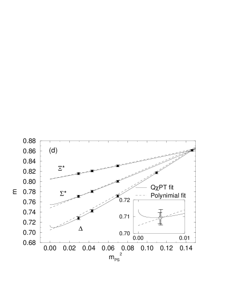
FIG. 1.: Chiral extrapolations for (a) pseudoscalar meson, (b) vector meson, (c) octet baryon and (d) decuplet baryon at $\beta=5.9$. The Q$\chi$PT and polynomial chiral fits are shown by solid and dashed lines. The insets are expanded displays for degenerate cases. In panel (a) AWI quark mass, $m_{q}^{AWI(0)}$ and linear chiral extrapolation are given (discussed in Sec. VII). In panels (c) and (d), we give data only for combinations of $(s_{1},u_{i},u_{i})$ and $(u_{i},u_{i},u_{i})$.

FIG. 2.: The same for Fig. 1 at $\beta=$ 6.10.

FIG. 3.: The same for Fig. 1 at $\beta=$ 6.25.

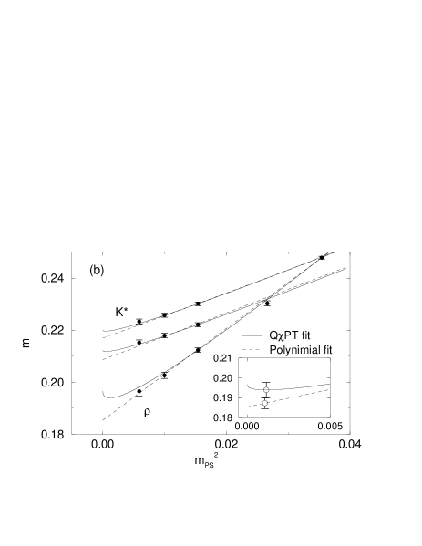
FIG. 4.: The same for Fig. 1 at $\beta=$ 6.47.

FIG. 5.: Continuum extrapolation of light hadron masses from $m_{K}$-input. Filled symbols and solid lines are the results from the Q$\chi$PT chiral fits, while open symbols and dashed lines are from the polynomial fits. Experimental values are shown by the stars.

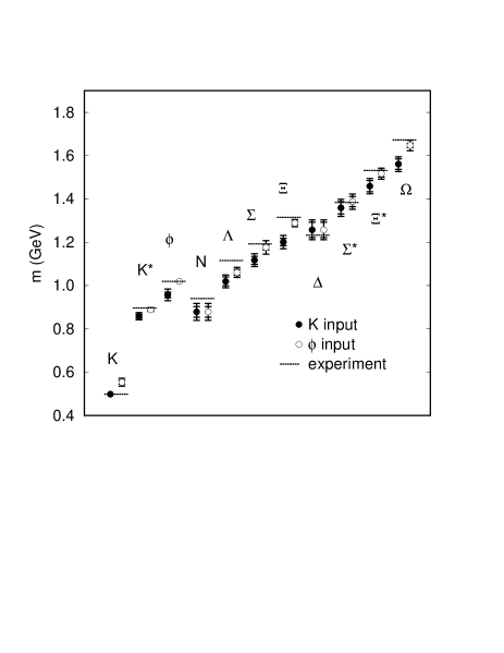
FIG. 6.: Quenched light hadron spectrum compared with experiment. The statistical error and the sum of the statistical and systematic errors are indicated.

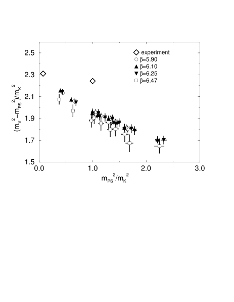
FIG. 7.: Hyperfine splitting of mesons normalized by $m_{K}$. Diamonds represent the experimental points corresponding to $(m_{PS},m_{V})=(m_{\pi},m_{\rho})$ and $(m_{K},m_{K}^{*})$, where the former is the input.

FIG. 8.: $J$ parameter. The star represents the experimental value.

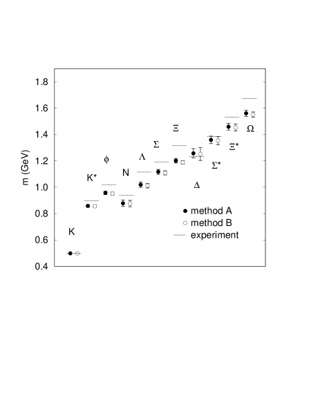
FIG. 9.: Comparison of the spectra from method A (black circles) and method B (open circles). $m_{K}$ is taken as input.

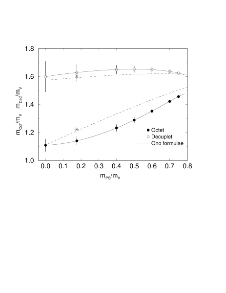
FIG. 10.: Edinburgh plot in the continuum limit. The stars represent experimental values. Dashed curves illustrate the phenomenological mass formulae by Ono [20].

FIG. 11.: The averaged mass of the up and down quarks and its continuum extrapolation. The leftmost point is the value extrapolated to the continuum limit.

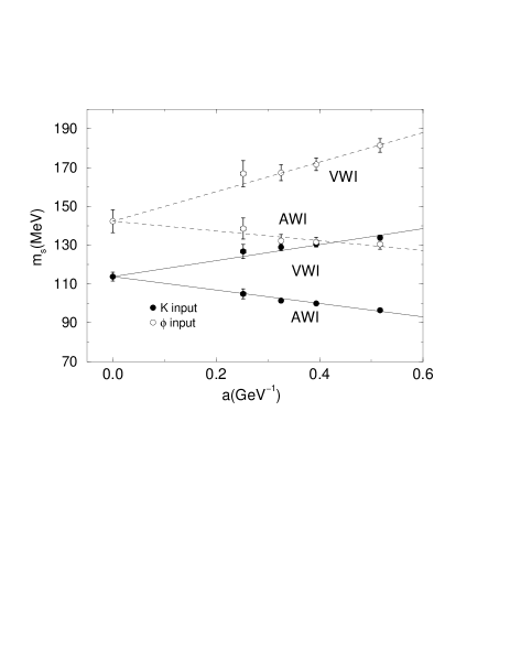
FIG. 12.: The strange quark masses and their continuum extrapolation. The leftmost points are the values extrapolated to the continuum limit.

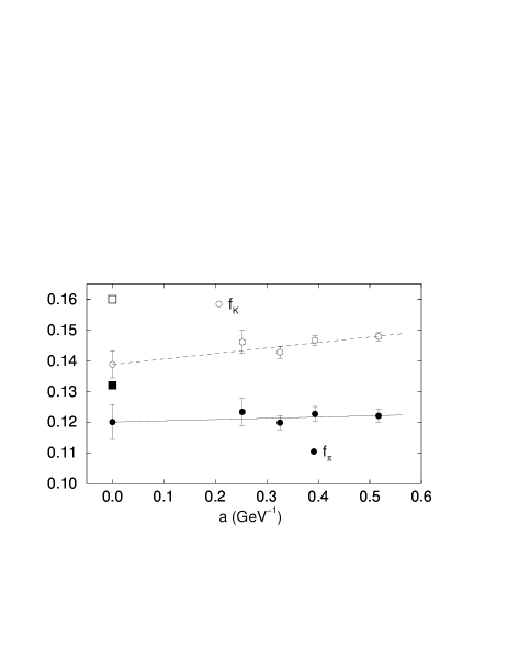
FIG. 13.: Continuum extrapolations of pseudoscalar meson decay constants $f_{\pi}$ and $f_{K}$ ($m_{K}$-input). Large squares at $a=0$ represent experimental values.

FIG. 14.: Continuum extrapolation of $f_{K}/f_{\pi}-1$ from the $m_{K}$-input. The square at $a=0$ represents the experimental value.

FIG. 15.: $F_{\rho}$ (top panel) and $F_{\phi}$ (bottom panel) as a function of $a$. Fits for the continuum extrapolation are also shown. Solid symbols are for non-perturbatively renormalized decay constants, and open symbols are for decay constants renormalized by tadpole-improved one-loop perturbation theory. Stars represent experimental values.

FIG. 16.: Typical effective masses obtained with various combinations of quark sources.

FIG. 17.: Effective mass plots of degenerate octet baryons at $m_{PS}/m_{V}\approx$ 0.75 (top), $m_{PS}/m_{V}\approx$ 0.6 (middle), and $m_{PS}/m_{V}\approx$ 0.4 (bottom) at $\beta=5.90$.

FIG. 18.: The same as Fig.17 at $\beta=$ 6.10.

FIG. 19.: The same as Fig.17 at $\beta=$ 6.25.

FIG. 20.: The same as Fig.17 at $\beta=$ 6.47.

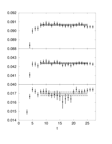
FIG. 21.: Effective mass plots for twice the AWI quark mass, $2m_{q}^{AWI(0)}$, at $\beta=5.90$ for the degenerate cases, corresponding to $m_{PS}/m_{V}\approx$ 0.75 (top), 0.6 (middle) and 0.4 (bottom).

FIG. 22.: The same as Fig. 21 at $\beta=$ 6.47.

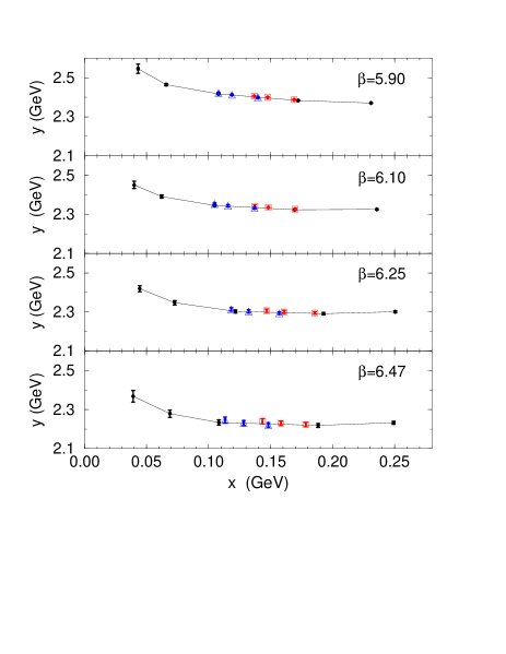
FIG. 23.: Deviations from the chiral relation $y\equiv m_{PS,12}^{2}/(m_{1}^{AWI}+m_{2}^{AWI})=$ constant. The horizontal axis is $x\equiv m_{1}^{AWI}+m_{2}^{AWI}$. Filled and open symbols represent degenerate and non-degenerate quark mass cases, respectively. The error from the lattice spacing is not included.

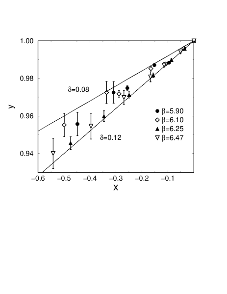
FIG. 24.: Test of quenched chiral logarithms for pseudoscalar meson masses.

FIG. 25.: Ratio test proposed in Ref. [5]. Data at $\beta=5.90$ are connected to the point $(0.0,1.0)$ to guide the eyes.

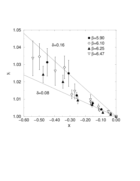
FIG. 26.: Ratio test of quenched chiral logarithms for pseudoscalar meson decay constants.

FIG. 27.: Degenerate hadron masses vs. $m_{PS}^{2}$ at $\beta$=5.9. The leftmost points are values extrapolated to the chiral limit, and the second ones from the left are those at the physical point. Fits from two types of chiral extrapolations based on Q$\chi$PT are shown. See text for details.

FIG. 28.: Light hadron spectrum from polynomial chiral fits.

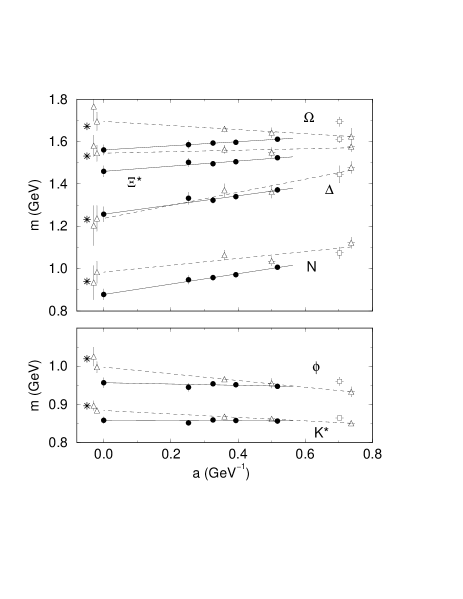
FIG. 29.: Comparison of our hadron masses (filled symbols) with those of Ref. [3] (open symbols). Open triangles (squares) are data obtained on lattices with $L_{s}a\approx 2.3$ fm ($L_{s}a\approx 3.4$ fm). Open symbols at $a\approx 0$ represent data on finite lattice (right) and those after finite size corrections (left). Experimental values are shown by stars.

FIG. 30.: The ratio $y=(m_{1}^{VWI}+m_{2}^{VWI})/(m_{1}^{AWI}+m_{2}^{AWI})$ as a function of $x=m_{1}^{AWI}+m_{2}^{AWI}$. Filled and open symbols are for degenerate and non-degenerate cases, respectively. $\kappa_{c}^{AWI}$ is used to calculate $m_{q_{i}}^{VWI}$. Errors from the lattice spacing are not included.

FIG. 31.: Chiral extrapolations of the quark mass based on the axial-vector Ward identity at $\beta=5.90$.

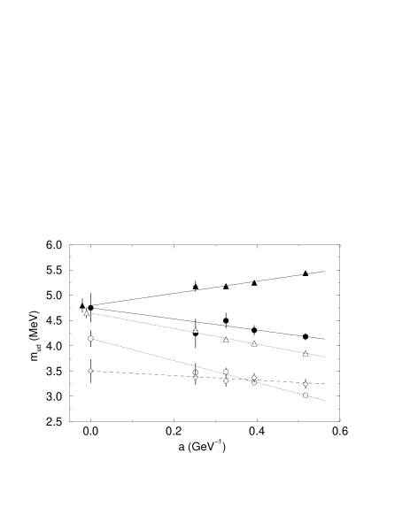
FIG. 32.: Comparison of the light quark masses determined from various chiral fits. The VWI (AWI) quark masses are shown by filled (open) symbols. Circles are results obtained from our main analysis, while triangles are from the alternative chiral fits discussed in the text. Open diamonds are obtained from fits to $m_{PS}^{2}$ as a function of $m_{q}^{AWI}$.

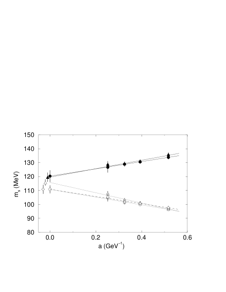
FIG. 33.: The same as Fig. 32 for the strange quark mass with $m_{K}$ input.

FIG. 34.: The same as Fig. 32 for the strange quark mass with $m_{\phi}$ input.

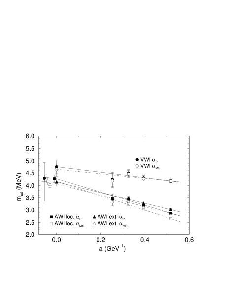
FIG. 35.: Comparison of the $u,d$ quark mass. Circles are the VWI quark masses. Triangles (squares) are the AWI quark masses derived from the extended (local) axial vector current. Filled (open) symbols indicate that masses are calculated using $\alpha_{P}$ ($\alpha_{\overline{\rm MS}}$). The leftmost data shows the result from a combined fit with the statistical error and the sum of statistical and systematic errors. See Sec. VII for detail.

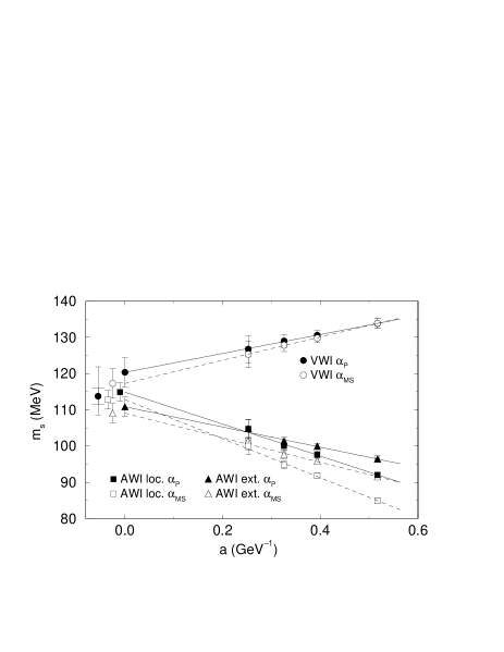
FIG. 36.: The same as Fig. 35 for $m_{s}$ with $m_{K}$ input.

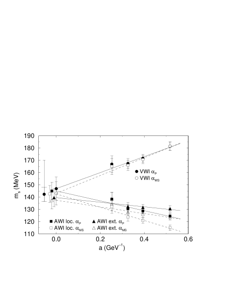
FIG. 37.: The same as Fig. 35 for $m_{s}$ with $m_{\phi}$ input.

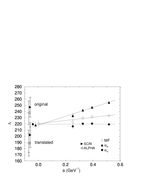
FIG. 38.: $\Lambda_{\overline{\rm MS}}$ vs $a$.

FIG. 39.: $\sqrt{\sigma}/m_{\rho}$ and $1/r_{0}m_{\rho}$ vs. $a$.

FIG. 40.: Examples of fits for Eq. (92) at $\beta$ = 6.10 in units of $10^{5}$. Three panels show the data for $m_{PS}/m_{V}\approx$ 0.75 (top), 0.6 (middle) and 0.4 (bottom).

FIG. 41.: Pseudoscalar meson decay constants versus $1/\kappa$ at $\beta=5.90$. Solid curves show chiral fits with quadratic polynomial (linear) for the degenerate (non-degenerate) case. Dashed line is for a linear fit to the degenerate case.

FIG. 42.: Ratios $\langle V^{C}V^{L}\rangle/\langle V^{L}V^{L}\rangle$ and fits to obtain $Z_{V}$ at $\beta=6.25$. Parameters are $m_{PS}/m_{V}\approx$ 0.75 (top), $m_{PS}/m_{V}\approx$ 0.6 (middle), and $m_{PS}/m_{V}\approx$ 0.4 (bottom) at $\beta=5.90$.

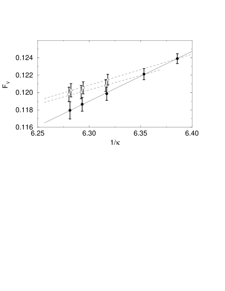
FIG. 43.: $F_{V}a$ vs. $1/\kappa$ at $\beta=5.90$ with chiral extrapolations. Non-degenerate data are slightly shifted in $x$ for clarity.

FIG. 44.: Degenerate masses and chiral fits in the continuum limit. $V=m_{V}^{(0.75)}$. See text for details.

FIG. 45.: Octet baryon mass in the chiral limit versus the lattice spacing. The leftmost point represents the value in the continuum limit but determined from the chiral fit in the continuum limit.

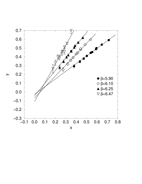
FIG. 46.: Ratio test for Q$\chi$PT formulae for degenerate vector mesons.

FIG. 47.: The same as Fig. 46, but for non-degenerate vector mesons.

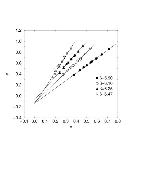
FIG. 48.: The same as Fig. 46, but for degenerate decuplet baryons.

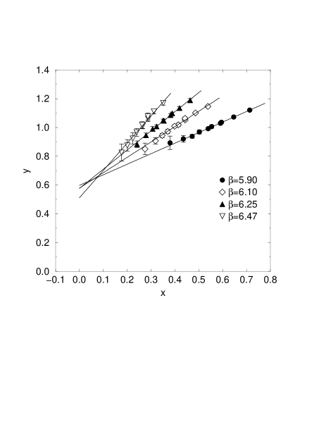
FIG. 49.: The same as Fig. 46, but for degenerate octet baryons.

REFERENCES

- [1] H. Hamber and G. Parisi, Phys. Rev. Lett. 47 (1981) 1792.
- [2] D. Weingarten, Phys. Lett. 109B (1982) 57.
- [3] F. Butler, H. Chen, J. Sexton, A. Vaccarino and D. Weingarten, Nucl. Phys. B430 (1994) 179.
- [4] S.R. Sharpe, Phys. Rev. D 46, 3146 (1992).
- [5] C.W. Bernard and M.F.L. Golterman, Phys. Rev. D 46, 853 (1992).
- [6] MILC Collaboration (C. Bernard et al.), Phys. Rev. Lett. 81, 3087 (1998).
- [7] Y. Iwasaki, Nucl. Phys. B (Proc. Suppl.) 53, 1007(1997); T. Boku, K. Itakura, H. Nakamura, K. Nakazawa, in Proceedings of ACM International Conference on Supercomputing’97, 108 (1997).
- [8] S. Aoki et al., Parallel Computing 25 (1999) 1243.
- [9] CP-PACS Collaboration (S. Aoki et al.), Phys. Rev. Lett. 84, 238 (2000).
- [10] CP-PACS Collaboration (S. Aoki et al.), Nucl. Phys. B (Proc. Suppl.) 60A, 14 (1998); 63, 161 (1998); 73, 189 (1999); R. Burkhalter, Nucl. Phys. B (Proc. Suppl.) 73, 3 (1999).
- [11] MILC Collaboration (C. Bernard et al.), Nucl. Phys. B (Proc. Suppl.) 60A, 3 (1998).
- [12] M. Lüscher, Commun. Math. Phys, 104, 177 (1986).
- [13] M. Fukugita et al., Phys. Lett. B294 380 (1992).
- [14] S. Aoki et al., Phys. Rev. D50 486 (1994).
- [15] N Cabibbo and E. Marinari, Phys. Lett. B119 (1982) 387; M.Okawa, Phys. Rev. Lett. 49 (1982) 353.
- [16] F.R. Brown and T. J. Woch, Phys. Rev. Lett.58 (1987) 2397.
- [17] M. Booth, G. Chiladze and A.F. Falk, Phys. Rev. D 55, 3092 (1997).
- [18] J.N. Labrenz and S.R. Sharpe, Phys. Rev. D 54, 4595 (1996).
- [19] P. Lacock and C. Michael, Phys. Rev. D52 (1995) 5213.
- [20] S. Ono, Phys. Rev. D17 888 (1978).
- [21] JLQCD Collaboration (S. Aoki et al.), Phys. Rev. Lett. 80, 5711 (1998).
- [22] M. Bochicchio et al., Nucl. Phys. B262, 331 (1985).
- [23] S. Itoh, Y. Iwasaki, Y. Oyanagi and T. Yoshié, Nucl. Phys. B274, 33 (1986).
- [24] J. Gasser and H. Leutwyler, Ann. Phys. 158 142 (1984) ; Nucl. Phys. B250 465 (1985).
- [25] S. Sharpe, private communication.
- [26] M.F.L. Golterman, private communication.
- [27] C.W. Bernard and M.F.L. Golterman, Nucl. Phys. B (Proc. Suppl.) 30, 217 (1993).
- [28] W. Bardeen, A. Duncan, E. Eichten and H. Thacker, Phys. Rev. D62, 114505 (2000).
- [29] QCDSF Collaboration (M. Göckeler et al.), Nucl. Phys. B (Proc. Suppl.) 83, 203(2000).
- [30] J. Heitger, R. Sommer, H. Wittig, Nucl. Phys. B588 377 (2000).
- [31] T. Bhattacharya, R. Gupta, G. Kilcup and S. Sharpe, Phys. Rev. D53, 6486 (1996).
- [32] S. Aoki, Nucl. Phys. (Proc. Suppl.) 94, 3 (2001).
- [33] A. Gonzalez Arroyo, G. Martinelli and F.J. Yndurain, Phys. Lett. B117 (1992) 437.
- [34] G. Martinelli and Y.C. Zhang, Phys. Lett. B125, 77 (1983).
- [35] G. Martinelli and Y.C. Zhang, Phys. Lett. B123, 433 (1983); B125, 77 (1983).
- [36] G.P. Lepage and P.B. Mackenzie, Phys. Rev. D48, 2250 (1993).
- [37] E. Franco and V. Lubicz, Nucl. Phys. B531, 641 (1998).
- [38] M. Lüscher and P. Weisz, Nucl. Phys. B452, 234 (1995).
- [39] O.V. Tarasov, A.A. Vladimirov, A.Yu. Zharkov, Phys. Lett. 93B, 429 (1980).
- [40] A. X. El-Khadra et al., Phys. Rev. Lett. 69 (1992) 729.
- [41] T.R. Klassen, Phys. Rev. D51, 5130 (1995).
- [42] M. Peter, Phys. Rev. Lett. 78, 602 (1997) ; Nucl. Phys. B501, 471 (1997).
- [43] B. Alles, M. Campostrini, A. Feo and H. Panagopoulos, Phys. Lett. B324, 433 (1994).
- [44] S.J. Brodsky, G.P. Lepage and P.B. Mackenzie, Phys. Rev. D28, 228 (1983).
- [45] R.G. Edwards, U.M. Heller and T.R. Klassen, Nucl. Phys. B517, 377 (1998).
- [46] ALPHA Collaboration (S. Capitani et al.), Nucl. Phys. B544, 669 (1999).
- [47] R. Sommer, Nucl. Phys. B411, 839 (1994).
- [48] C.R. Allton, hep-lat/9610016.
- [49] G.P. Lepage, Nucl. Phys. B (Proc.Suppl.) 26 (1992) 45; A.S. Kronfeld, Nucl. Phys. B (Proc.Suppl.) 30 (1993) 445; P.B. Mackenzie, Nucl. Phys. B (Proc.Suppl.) 30 (1993) 35.
- [50] L. Maiani and G. Martinelli, Phys. Lett. B178 (1986) 265.
- [51] CP-PACS Collaboration (A. Ali-Khan et al), Phys. Rev. Lett. 85 (2000) 4674; Phys. Rev. D65 (2001) 054505.
- [52] H. Mino, unpublished.
- [53] QCDPAX Collaboration (Y. Iwasaki et al.), Phys. Rev. D53 (1996) 6443.