Numerical simulation tests with light dynamical quarks

Abstract

Two degenerate flavours of quarks are simulated with small masses down to about one fifth of the strange quark mass by using the two-step multi-boson (TSMB) algorithm. The lattice size is $8^{3}\cdot 16$ with lattice spacing about $a\simeq 0.27\,{\rm fm}$ which is not far from the $N_{t}=4$ thermodynamical cross-over line. Autocorrelations of different physical quantities are estimated as a function of the quark mass. The eigenvalue spectra of the Wilson-Dirac operator are investigated.

1 Introduction

The question about the computational cost of dynamical quark simulations is a central issue in lattice gauge theory. Existing unquenched simulations are typically done in a region where the quarks are not light enough, in most cases – especially in case of Wilson-type quarks – with two light quark flavours ($u$ and $d$) having masses larger than half of the strange quark mass ($m_{ud}>\frac{1}{2}m_{s}$). The physical masses of $u$- and $d$-quarks are so small that in the foreseeable future simulations can only be carried out at somewhat higher masses. In order to extrapolate the results to the physical masses chiral perturbation theory based on the low energy chiral effective Lagrangian can be used. However the systematic errors can only be controlled if the dynamical quark masses in the simulations are close enough to the physical point. For instance, in case of partially quenched simulations to determine the low energy constants in the chiral effective Lagrangian of QCD we would like to reach at least $m_{ud}\leq\frac{1}{4}m_{s}$ Sharpe:SHORESH.

Going to light quark masses in unquenched QCD simulations is a great challenge for computations because known algorithms have a substantial slowing down towards small quark masses. The present status has been recently summarized by the contributors to the panel discussion at the Berlin lattice conference Christ:BERLIN; Gottlieb:BERLIN; Jansen:BERLIN; Lippert:BERLIN; Ukawa:BERLIN; Wittig:BERLIN. Inspired by the results presented there the computational cost of a simulation with two light quarks will be parametrized in the present paper as

$$C=F\;(r_{0}m_{\pi})^{-z_{\pi}}\left(\frac{L}{a}\right)^{z_{L}}\left(\frac{r_{0}}{a}\right)^{z_{a}}\ .$$ (1)

Here $r_{0}$ is a physical length, for instance the Sommer scale parameter Sommer:SCALE, $m_{\pi}$ the pion mass, $L$ the lattice extension and $a$ the lattice spacing. The powers $z_{\pi,L,a}$ and the overall constant $F$ are empirically determined. The value of the constant factor $F$ depends on the precise definition of “cost” Frezzotti:BENCHMARK. For instance, one can consider the number of floating point operations in one autocorrelation length of some important quantity, or the number of fermion-matrix-vector-multiplications necessary for achieving a given error of a quantity. Of course, the cost also depends on the particular choice of lattice action and of the dynamical fermion algorithm which should be optimized.

An alternative parametrization can be obtained from the one in (1) by replacing the powers of $r_{0}m_{\pi}$ by those of $m_{\pi}/m_{\rho}$. In fact, the results of the CP-PACS, JLQCD Collaboration have been presented by A. Ukawa at the Berlin lattice conference Ukawa:BERLIN in this form:

$$C_{U}=F_{U}\;\left(\frac{m_{\pi}}{m_{\rho}}\right)^{-z_{\pi\rho}}\left(\frac{L}{a}\right)^{z_{L}}\left(\frac{r_{0}}{a}\right)^{z_{a}}\ ,$$ (2)

$$F_{U}=5.9\cdot 10^{6}\,{\rm flop}$$ (3)

$$z_{\pi\rho}=6\ ,\hskip 10.00002ptz_{L}=5\ ,\hskip 10.00002ptz_{a}=2\ .$$ (4)

Since the determination of the $\rho$ meson mass is difficult for light quarks when the decay $\rho\to\pi\pi$ is allowed, we prefer the form in (1). Other parametrizations used for Wilson-type quarks Lippert:BERLIN; Wittig:BERLIN are given under the assumption that $z_{\pi}=z_{a}\equiv z_{a\pi}$ when in (1) the physical length parameter $r_{0}$ disappears.

In the present paper we report on the results of extended test runs with the simple Wilson fermion action using the two-step multi-boson algorithm Montvay:TSMB in order to determine the quark mass dependence of the computational cost of dynamical Monte Carlo simulations with two light flavours in the region $m_{ud}\geq\frac{1}{5}m_{s}$. For the definition of the quark mass the dimensionless quantity

$$M_{r}\equiv(r_{0}m_{\pi})^{2}$$ (5)

is used, which already appears in (1). This is a possible definition for small quark masses because for $m_{q}\to 0$ the pion mass behaves as $m_{\pi}\propto\sqrt{m_{q}}$. For defining the value of $M_{r}$ which corresponds to the strange quark mass one can use unquenched $N_{f}=2$ lattice data. For instance, the experimental value of the $\Omega^{-}$ baryon mass $m_{\Omega^{-}}=1.672\,{\rm GeV}$ and $r_{0}=0.5\,{\rm fm}$ give $r_{0}m_{\Omega^{-}}=4.237$. Interpolating CP-PACS results AliKhan:NF2SPECT for the $\Delta$ baryon mass at their largest $\beta$ value $\beta=2.20$ between $\kappa=0.1363$ and $\kappa=0.1368$ one can match $r_{0}m_{\Delta}=4.237$ if their pion mass is $r_{0}m_{\pi}\simeq 1.76$. This gives for the strange quark mass $M_{r,strange}\simeq 3.1$. Of course, there are also other ways to estimate $M_{r,strange}$ which might give slightly different values. In the present paper, without attempting to really compute the strange quark mass, we shall stick to the operational definition

$$M_{r,strange}\equiv 3.1\ .$$ (6)

The Monte Carlo simulations are done near the $N_{t}=4$ thermodynamical cross-over line that is for $a\simeq 0.27\,{\rm fm}$. The lattice size is $8^{3}\cdot 16$ implying a physical lattice extension $L\simeq 2.2\,{\rm fm}$. Later on we shall also extend our investigations to $12^{3}\cdot 24$ and $16^{3}\cdot 32$ lattices. Our present studies can be considered as complementary to the ones on larger lattices (closer to the continuum limit) but at larger quark masses (typically $m_{ud}\geq\frac{1}{2}m_{s}$) Christ:BERLIN-Wittig:BERLIN.

In addition to obtaining estimates of autocorrelation lengths as a function of the quark mass we also performed a detailed study of the small eigenvalue spectra both for the hermitean and non-hermitean Wilson-Dirac fermion matrix. Besides giving important qualitative information about quark dynamics this also allows to clear the issue of the sign problem of the quark determinant. For an odd number of Wilson-type quark flavours the fermion determinant can have both signs because there might be some eigenvalues (of the non-hermitean fermion matrix) on the negative real axis. Since for importance sampling a positive measure is required, the determinant sign can only be taken into account in a measurement reweighting step. A strongly fluctuating determinant sign is a potential danger for the effectiveness of the Monte Carlo simulation because cancellations can occur resulting in an unacceptable increase of statistical errors. We actually study this question here with two degenerate quark flavours ($N_{f}=2$) where in the path integral the square of the fermion determinant appears and hence the sign is irrelevant. But our two quarks are much lighter than the physical $s$-quark. Therefore the statistical insignificance of negative eigenvalues in this case hints towards the absence of the sign problem in the physical case of $N_{f}=2+1$ quark flavours, when the sign of the $s$-quark determinant could, in principle, cause a problem.

The plan of this paper is as follows: in the next section we shortly introduce the parameters of the TSMB algorithm and give some details of our implementation on different computers. In section 3 the autocorrelations are investigated for some basic quantities such as the average plaquette and the pion mass. Section 4 contains a detailed study of the small eigenvalue spectra of the fermion matrix. The last section is devoted to discussion and conclusions.

2 The TSMB algorithm

We use in this study the two-step multi-boson (TSMB) algorithm which has been originally developed for Monte Carlo simulations of the supersymmetric Yang-Mills theory Montvay:TSMB but it can also be applied more generally Montvay:QCD.

2.1 Algorithmic parameters

TSMB is based on a representation of the fermion determinant in the form

$$\left|\det(Q)\right|^{N_{f}}\;\simeq\;\frac{1}{\det P^{(1)}_{n_{1}}(\tilde{Q}^{2})\det P^{(2)}_{n_{2}}(\tilde{Q}^{2})}\ .$$ (7)

Here $N_{f}$ denotes the number of fermion flavours and $Q$ is the fermion matrix, which in the present paper is equal to the Wilson-Dirac matrix

$$Q_{ys,xr}\equiv\delta_{yx}\delta_{sr}-\ \ \ \ \ \ \ \ \ \ \ \ \ \ \ \ \ \ \ \$$ (8)

$$\kappa\sum_{\mu=1}^{4}\left[\delta_{y,x+\hat{\mu}}(1+\gamma_{\mu})U_{sr,x\mu}+\delta_{y+\hat{\mu},x}(1-\gamma_{\mu})U^{\dagger}_{sr,y\mu}\right]$$

with $x,y$ denoting lattice sites, $r,s$ colour (triplet) indices, $\hat{\mu}$ the unit lattice vector in direction $\mu$, $U_{x\mu}\in{\rm SU}(3)$ gauge link matrices and $\kappa$ the hopping parameter. The hermitean Wilson-Dirac fermion matrix is defined as usual by

$$\tilde{Q}\equiv\gamma_{5}Q=\tilde{Q}^{\dagger}\ .$$ (9)

The polynomial approximations in (7) satisfy

$$P^{(1)}_{n_{1}}(x) \simeq x^{-N_{f}/2}\ ,$$

$$\lim_{n_{2}\to\infty}P^{(1)}_{n_{1}}(x)P^{(2)}_{n_{2}}(x) = x^{-N_{f}/2}\ ,\hskip 20.00003ptx\in[\epsilon,\lambda]$$ (10)

where the interval $[\epsilon,\lambda]$ covers the spectrum of the squared hermitean fermion matrix $\tilde{Q}^{2}$ on a typical gauge configuration. The first polynomial $P^{(1)}$ is a crude approximation with relatively low order. It is used in the multi-boson representation of fermion determinants Luscher:MB. The second polynomial $P^{(2)}$ is a correction factor which is taken into account in the gauge field updating by a global accept-reject step. For this a polynomial approximation of the inverse square root of $P^{(2)}$ is also needed:

$$P^{(3)}_{n_{3}}(x)\simeq P^{(2)}_{n_{2}}(x)^{-\frac{1}{2}}\ .$$ (11)

The limit $n_{2}\to\infty$ can be taken in the computed expectation values if one produces several update sequences with increasing $n_{2}$ or, more conveniently, one can keep $n_{2}$ fixed at some sufficiently large value for a good approximation and introduce a further polynomial $P^{(4)}$ satisfying

$$\lim_{n_{4}\to\infty}P^{(1)}_{n_{1}}(x)P^{(2)}_{n_{2}}(x)P^{(4)}_{n_{4}}(x)=x^{-N_{f}/2}\ .$$ (12)

$P^{(4)}$ can be taken into account by reweighting the gauge configurations during the evaluation of expectation values. In most cases the order $n_{2}$ of $P^{(2)}_{n_{2}}$ can be chosen high enough such that the reweighting correction has a negligible effect on expectation values. In any case the evaluation of the reweighting factors is useful because it shows whether or not the two-step approximation in (2.1) is good enough. For a recent summary of some details of TSMB and for references see section 3 of Montvay:SYMREV.

The Monte Carlo integration of the path integral is performed by averaging over a sequence (Markov chain) of multi-boson and gauge field configurations. The $n_{1}$ multi-boson fields ($\Phi$) and gauge fields ($U$) are updated in repeated update cycles consisting of several sweeps over the multi-boson fields and gauge field. For the multi-boson fields we use (local) heatbath and overrelaxation as well as global quasi-heatbath deForcrand:QUASIHEAT sweeps. For the gauge field update heatbath and overrelaxation sweeps are alternated. After several gauge field sweeps a global Metropolis accept-reject correction step is performed by the polynomials $P^{(2)}$ and $P^{(3)}$. The update sequence within a cycle is subject to optimization with the goal to decrease autocorrelations. We tried several kinds of update sequences within an update cycle. A typical sequence was: 3 $\Phi$-overrelaxations, 1 $\Phi$-heatbath, 12 $U$-overrelaxation, global $U$-Metropolis, 3 $\Phi$-overrelaxations, 1 $\Phi$-heatbath, 6 $U$-heatbath, global $U$-Metropolis. In every 10-th cycle the first $\Phi$-overrelaxation-$\Phi$-heatbath combination was replaced by a global quasi-heatbath.

2.2 Implementation and performance

We have implementations of the updating and measurement programs in TAOmille for the APEmille and in C++/ MPI. The latter implementation is usable on many different architectures as long as they provide a C++ compiler and, in case of parallel computers, support MPI. In the updating program the computing time is dominated by the fermion-matrix-vector-multiplications (MVMs), $2\cdot(n_{2}+n_{3})$ of them are needed for the correction step and ${\cal O}(100\cdot n_{1})$ for the global heatbath and quasi-heatbath deForcrand:QUASIHEAT. Altogether they make up $60\%-80\%$ of the computing time. In the most interesting regions of small quark masses the program is dominated by the MVMs even more strongly. The same is true for the measurement program, where smearing and calculation of simple Wilson loops takes only a few percent of the time. It is therefore of the utmost importance to improve the performance of the MVM routines, both preconditioned (for the correction step and the measurements) and non-preconditioned (for the global heatbath). This has been done for the APEmille, the Cray T3E with the KAI C++ compiler, and for a multi-node Pentium-4 cluster here also exploiting the possibilities of SSE and SSE2 instructions. Results are given in table 1. Note that an important feature of the SSE instructions is that in single precision the peak performance is doubled compared to double precision. The performance numbers in table 1 are substantially influenced by the communication costs among computing nodes. Without communications the numbers both for APEmille and P4-cluster would be almost a factor of two higher. On larger volumes than those considered here communication will have less influence on the performance.

Table 1: Performance of the matrix-vector-multiplication in MFlops and percent relative to peak performance on one board (8 nodes) on the APEmille and on 8 processors on the T3E and P4-cluster for a $8^{3}\cdot 16$ lattice.

	APEmille	T3E-1200	P4-1700
32 bit	1008 (23.9%)	912 (9.5%)	4322 (7.9%)
64 bit		712 (7.4%)	2087 (7.7%)

Since the matrix multiplications dominate the computing time it is reasonable to express e.g. autocorrelations in units of MVMs. The remaining part of the computation is given by the local updates. These are composed of parts which can be essentially thought of as pieces of MVMs, too. As a result the following approximate formula for the total amount of MVMs needed for one update cycle is obtained:

$$N_{MVM}/\mbox{cycle}\;\simeq\;6\,(n_{1}N_{\Phi}+N_{U})+2\,(n_{2}+n_{3})N_{C}+I_{G}F_{G}\ .$$ (13)

Here $N_{\Phi}$ is the number of local bosonic sweeps per update cycle, $N_{U}$ the number of local gauge sweeps, $N_{C}$ the number global Metropolis accept-reject correction steps, and $I_{G}$ and $F_{G}$ give the number of MVMs and frequency of the global heatbath.

For data from APEmille and Cray the estimate of the cost of the local updates obtained from (13) agrees with the actual costs up to $5\%$. Therefore the final costs in units of MVM based on (13) are not much influenced by the approximation. This is not true for the data presented for the P4-1700 system, since in this case the matrix multiplication and the local updates are not treated homogeneously. Indeed the former is written in assembler using SSE/SSE2 instructions while our code for the local updates is written in C++ and compiled with the g++ compiler. As a result, the estimate for the cost of the local updates is in this case underestimated by about a factor three. Still we take the above formula as a reference when tuning the parameters because the number of MVMs is more generally applicable as it does not depend on implementation details. In addition, in the future the local updates could be rewritten by using SSE/SSE2 instructions, too, so eliminating the non-homogeneity with the MVMs.

It is sometimes interesting to convert the number of MVMs into the number of floating point operations. On our $8^{3}\cdot 16$ lattice this conversion is approximately

$$1\;{\rm MVM}\;\simeq\;1.1\cdot 10^{7}\;{\rm flop}\ .$$ (14)

3 Autocorrelations at small quark masses

The bare parameters of the QCD lattice action with Wilson quarks ($\beta$ for the SU(3) gauge coupling and $\kappa$ for the hopping parameter of two degenerate quarks) have to be tuned properly in order to obtain the desired parameters in the Monte Carlo simulations. We are interested in the quark mass dependence of the simulation cost of hadron spectroscopy applications, therefore we want to keep the physical volume of our lattices sufficiently large and (approximately) constant. For a $8^{3}\cdot 16$ lattice, a lattice spacing $a\simeq 0.27\,{\rm fm}$ implies a lattice extension of $L\simeq 2.2\,{\rm fm}$ which is a reasonable starting point for spectroscopy. Previous Monte Carlo simulations with $N_{f}=2$ Wilson quarks Iwasaki:NT4; Blum:NT6 showed that this kind of lattice spacing is realized near the $N_{t}=4$ and $N_{t}=6$ thermodynamical transition lines which, therefore, provide a good orientation. We started our simulations at a relatively large quark mass on the $N_{t}=4$ transition line and then tuned $\beta$ and $\kappa$ towards smaller quark masses keeping $r_{0}/a$ approximately constant. A summary of simulation points is given in table 2 where some important algorithmic parameters of the TSMB are also collected.

Table 2: Bare couplings, parameters of the TSMB algorithm as defined in section 2.1 and total statistics in 1000 update cycles ($U_{k}$) of our runs.

run	$\beta$	$\kappa$	$n_{1}$	$n_{2}$	$n_{3}$	$n_{4}$	$\lambda$	$\epsilon$	$U_{k}$
$(a)$	5.28	0.160	20	40	70	100	2.8	1.75 $\cdot 10^{-2}$	80
$(b)$	5.04	0.174	28	90	120	150	3.0	3.75 $\cdot 10^{-3}$	33
$(c)$	4.84	0.186	38	190	240	300	3.6	1.44 $\cdot 10^{-3}$	31
$(d)$	4.80	0.188	44	240	300	300	3.6	7.2 $\cdot 10^{-4}$	12
$(e)$	4.76	0.190	44	360	380	500	3.6	2.7 $\cdot 10^{-4}$	144
$(f)$	4.80	0.190	44	360	380	500	3.6	2.7 $\cdot 10^{-4}$	224
$(g)$	4.72	0.193	52	600	750	800	3.6	0.9 $\cdot 10^{-4}$	196
$(h)$	4.68	0.195	66	900	1200	1100	3.6	3.6 $\cdot 10^{-5}$	200
$(i)$	4.64	0.197	72	1200	1500	1400	3.6	1.8 $\cdot 10^{-5}$	110
$(j)$	4.64	0.1975	72	1200	1350	1400	4.0	2.0 $\cdot 10^{-5}$	4

Most of the runs have been done with 32-bit arithmetics. Exceptions are run $(j)$ and about 10% of the statistics in run $(h)$ where 64-bit arithmetics was used. In general, on the $8^{3}\cdot 16$ lattice it is not expected that single precision makes any difference. In fact, the double precision results in run $(h)$ were compatible within errors with the single precision ones.

3.1 Physical quantities

In order to monitor lattice spacing and quark mass one has to determine some physical quantities containing the necessary information. As discussed before, we define the physical distance scale from the value of the Sommer scale parameter $r_{0}$. Once $r_{0}$ in lattice units is known one can transform any dimensionful quantity, for instance the pion mass $m_{\pi}$, from lattice to physical units. Therefore a careful determination of $r_{0}/a$ is important. For a dimensionless quark mass parameter one can use $M_{r}$ as defined in (5): $M_{r}=(r_{0}/a\cdot am_{\pi})^{2}$. In addition, we also measured some other quantities like $f_{\pi}$, $m_{\rho}$ and another definition of the quark mass $m_{q}$ for obtaining a broader basis for orientation. In the next subsections the procedures for extracting these quantities will be described in detail.

3.1.1 Masses and amplitudes

In order to extract masses and amplitudes we compute the zero-momentum two-point functions depending on the time-slice distance $(x_{0}-y_{0})$

$$C_{XY}(x_{0}-y_{0})=\frac{1}{V_{s}}\sum_{\bf x,y}\langle X^{\dagger}(x)Y(y)\rangle\ ,$$ (15)

with $x\equiv(x_{0},{\bf x})$ and

$$X(x) = Y(x)=P_{5}(x)\equiv\bar{q^{\prime}}(x)\gamma_{5}q(x)\,\ \ \ \ \ \ (C_{PP}(x_{0}-y_{0})),$$

$$X(x) = Y(x)=A_{0}(x)\equiv\bar{q^{\prime}}(x)\gamma_{5}\gamma_{0}q(x)\ \ \ \ (C_{AA}(x_{0}-y_{0})),$$

$$X(x) = Y(x)=V_{i}(x)\equiv\bar{q^{\prime}}(x)\gamma_{5}\gamma_{i}q(x)\,\,\ \ \ \ (C_{V_{i}V_{i}}(x_{0}-y_{0}));$$

we also consider the mixed correlator with

$$X(x)=A_{0}(x)\ ,\ \ \ \ Y(x)=P_{5}(x)\ \ \ \ \ \ \ \ \ \ \ \ \,(C_{AP}(x_{0}-y_{0}))\ \ .$$

Exploiting translation invariance we pick the source $y$ in (15) at random over the lattice. Taking into account correlations between different time-slices, one sees that this procedure is optimal for the ratio computational cost / final statistical error for hadronic observables.

Masses and amplitudes are in general obtained from the asymptotic behaviour of the correlators:

$$C_{XY}(T) = \frac{\xi_{XY}^{2}}{2m_{p}}\,\,(e^{-m_{p}T}+(-1)^{X+Y}e^{-m_{p}(L_{t}-T)})$$ (16)

$$\xi_{XY} = \sqrt{\langle 0|X(0)|p\rangle\langle 0|Y(0)|p\rangle}\ ,$$ (17)

where $|p\rangle$ is the zero-momentum state of the particle associated with the operators $X(x)$ and $Y(x)$, $m_{p}$ the corresponding mass and $(-1)^{X(Y)}$ the time-parity of $X(Y)(x)$. We determine parameters $m_{p}$ and $\xi_{XY}$ by global fitting over a range of time-slice distances (after time- symmetrization) $T\in[T_{min},L_{t}/2]$. We find the optimal value for $T_{min}$ by checking the behaviour of the effective local mass $m_{eff}(T)$. The latter is implicitly defined by the relation

$$\frac{C_{XY}(T)}{C_{XY}(T+1)}=$$ (18)

$$\,\,\,\,\frac{e^{-m_{eff}\,(T)T}+(-1)^{X+Y}e^{-m_{eff}(T)\,(L_{t}-T)}}{e^{-m_{eff}\,(T)(T+1)}+(-1)^{X+Y}e^{-m_{eff}(T)\,(L_{t}-T-1)}}\ .$$

The value of $T_{min}$ is fixed by the onset of the plateau for $m_{eff}(T)$ as a function of $T$. The plateau-value for the effective mass is always consistent with the result from the global fit procedure. The latter gives however the most precise determination.

A typical problem associated with small quark masses is a delayed asymptotic behaviour for correlators (i.e. a larger $T_{min}$) resulting in large errors for the hadronic observables. This problem was solved by applying Jacobi smearing Allton:JAC on both source and sink. Jacobi smearing was applied in a different context Campos:GLUINO; Farchioni:SUSYWTI in the same situation of light fermionic degrees of freedom, and it showed to improve the overlap of the hadronic operators with the bound-state. Amplitudes and decay constants have been determined from correlators with local operators.

We determine the pion mass $m_{\pi}$ from the asymptotic behaviour of the correlator $C_{PP}(T)$. From $C_{PP}(T)$ one can also extract the amplitude $g_{\pi}=\langle 0|P_{5}(0)|\pi\rangle$ by identifying $g_{\pi}=\xi_{PP}$. The $\rho$ meson mass $m_{\rho}$ is determined from the asymptotic behaviour of the correlator

$$C_{VV}(T)=\frac{1}{3}\sum_{i=1}^{3}\>C_{V_{i}V_{i}}(T)\ .$$ (19)

For the determination of the pion decay constant $f_{\pi}\equiv m_{\pi}^{-1}\,\langle 0|A_{0}(0)|\pi\rangle$ we apply two different methods. In the first, the amplitude $\langle 0|A_{0}(0)|\pi\rangle$ is obtained by fitting the asymptotic behaviour of the correlator $C_{AA}(T)$ while the pion mass is the one coming from $C_{PP}(T)$. In the second method Baxter:QUEN, we fit the amplitude-ratio

$$r_{AP}=\frac{\langle 0|A_{0}(0)|\pi\rangle}{\langle 0|P_{5}(0)|\pi\rangle}$$ (20)

by using the asymptotic behaviour

$$\frac{C_{AP}(T)}{C_{PP}(T)}=r_{AP}\tanh[m_{\pi}(L_{t}/2-T)]$$ (21)

where $m_{\pi}$ is fixed at the best-fit value from $C_{PP}(T)$. The determination of $f_{\pi}$ is then obtained from the relation

$$f_{\pi}=m_{\pi}^{-1}r_{AP}\,g_{\pi}$$ (22)

using for $g_{\pi}$ the determination from $C_{PP}(T)$. In the region of large and moderate quark masses the second method gives by far the most precise determination of $f_{\pi}$. This is generally no more true for very light quarks where data are highly correlated. Here the best determination was picked from the two different methods on a case-by-case basis.

Using the above determinations we can extract the quark mass defined by the PCAC relation

$$m^{PCAC}_{q}=\frac{f_{\pi}}{2g_{\pi}}\,m_{\pi}^{2}\ .$$ (23)

The PCAC quark mass gives us a second definition of the physical quark mass alternative to (5)

$$\mu_{r}\equiv r_{0}m^{PCAC}_{q}\ .$$ (24)

We estimated statistical errors on hadron quantities by applying the Jackknife procedure on blocks of data of increasing size. The same procedure is applied also for the Sommer scale parameter (see next subsection). This method provides us with a definition of the integrated autocorrelation $\tau_{int}$ of the pion mass. Autocorrelations in general will be discussed in section (3.2). The results for the hadronic quantities are listed in table 3.

3.1.2 Sommer scale parameter

There are several phenomenological models that can be used to get an estimate for the Sommer scale parameter $r_{0}$ in nature, and most of them point towards a value of $r_{0}\simeq 0.49\mbox{fm}$. On the lattice $r_{0}/a$ can be calculated from the static quark potential, which is in turn determined from Wilson loops. The basic idea is simple, but since we want to match all our results to this parameter it is crucial to get a precise determination. To achieve this we follow the method proposed by Michael and collaborators Michael:R0; Perantonis:R0 and some details in Allton:R0.

Using the variational approach of Luscher:R0 we get matrices $W_{ij}(r,t)$ consisting of $r\times t$ loops of smeared gauge links, where our smearing technique of choice is APE-smearing (indices $i,j$ label the level of smearing). We use for our determinations two and six or two, four and six levels of smearing and symmetrize the matrices $W_{ij}$. The ratio staple/link is set to $\alpha=0.45$.

From the solutions to

$$W_{ij}({\bf r},t)\phi({\bf r})_{j}^{(k)} = \lambda^{(k)}({\bf r};t,t_{0})W_{ij}({\bf r},t_{0})\phi({\bf r})_{j}^{(k)},$$

$$i,j,k = 0,1(,2)$$ (25)

one gets the eigenvector $\phi({\bf r})_{j}^{(0)}$ for the largest eigenvalue $\lambda^{(0)}({\bf r};t=t_{0}+1,t_{0})$. This equation is solved by transforming it into an ordinary eigenvalue equation, where several ways are possible:

$$W({\bf r},t_{0})^{-1}W({\bf r},t)\phi=\lambda\phi$$ (26)

$$W({\bf r},t)W({\bf r},t_{0})^{-1}(W({\bf r},t_{0})\phi)=\lambda(W({\bf r},t_{0})\phi)$$ (27)

$$W({\bf r},t_{0})^{-1/2}W({\bf r},t)W({\bf r},t_{0})^{-1/2}(W({\bf r},t_{0})^{1/2}\phi)$$

$$=\lambda(W({\bf r},t_{0})^{1/2}\phi)\ .$$ (28)

In the literature Luscher:R0 the third version has been used. However this can only be done with extremely good statistics. Otherwise it is possible that, due to statistical fluctuations, the matrix $W_{ij}$ gets negative eigenvalues making the (real) square root impossible. We checked that the first two versions give numerically exactly the same result. For the final determinations we choose the first version (26), where one has to be careful about the fact that $W({\bf r},t_{0})^{-1}W({\bf r},t)$ has no longer to be symmetric, complicating the calculation of the corresponding eigenvectors.

Once the eigenvector $\phi({\bf r})_{j}^{(0)}$ has been obtained, we can project the matrix $W_{ij}$ to the ground state:

$$\tilde{W}_{0}({\bf r},t)=\phi({\bf r})_{i}^{(0)}W_{ij}({\bf r},t)\phi({\bf r})_{j}^{(0)}\ .$$ (29)

This correlator leads to good estimates of the ground state energy

$$\tilde{E}_{0}({\bf r},t)=\ln\left(\frac{\tilde{W}_{0}({\bf r},t)}{\tilde{W}_{0}({\bf r},t+1)}\right)\ .$$ (30)

The potential V(r) is estimated by averaging $E_{0}({\bf r},t)/t$ over time extensions $t$ with $t\geq 1$ and weight given by the Jackknife error. Compared to some other methods this way of extracting the potential seems to give the most reliable estimates with smallest error bars.

The Sommer scale parameter is defined in terms of the potential as

$$r_{0}^{2}\left.\frac{\mbox{d}V}{\mbox{d}r}\right|_{r_{0}}=1.65\ .$$ (31)

Having a reliable static quark potential we can follow Edwards:R0 by fitting the potential to

$$V({\bf r})=V_{0}+\sigma r-e[\frac{1}{{\bf r}}]$$ (32)

with $r=|{\bf r}|$ and $[\frac{1}{{\bf r}}]$ being the tree-level lattice Coulomb term

$$[\frac{1}{{\bf r}}]=4\pi\int^{\pi}_{-\pi}\!\!\frac{\mbox{d}^{3}{\bf k}}{(2\pi)^{3}}\frac{\cos({\bf k}\cdot{\bf r})}{4\sum_{j=1}^{3}\sin^{2}(k_{j}/2)}\ .$$ (33)

Due to the small lattice size we had to drop in (32) the additional correction term $f\cdot\left([\frac{1}{{\bf r}}]-\frac{1}{r}\right)$, which could have been used to estimate ${\cal O}(a)$ effects, fixing $e=\pi/12$. Bringing together the above equations we extract $r_{0}$ from

$$r_{0}=\sqrt{\frac{1.65-e}{\sigma}}\ .$$ (34)

3.2 Autocorrelations

The “cost” of numerical simulations can be expressed in terms of the necessary number of arithmetic operations for obtaining during the Monte Carlo update process a new “independent” gauge field configuration. The real cost can be then easily calculated once the price of e.g. a floating point operation is known. For a definition of the independence of a new configuration the integrated autocorrelation $\tau_{int}$ is used. (For a general reference see Montvay:BOOK.) $\tau_{int}$ does depend on the particular quantity it refers to. Of course, it is reasonable to choose an “important” quantity as, for instance, the pion mass but simple averages characterizing the gauge field such as the plaquette average are also often considered.

In case of the TSMB algorithm a peculiar feature is the reweighting step correcting for the imperfection of polynomial approximations. As will be discussed in the next subsection, in most of our runs this correction is totally negligible but even in these cases it is important to perform the reweighting on a small subsample of configurations in order to check that the used polynomials are precise enough. In some cases, especially for very small quark masses, there are a few exceptional configurations with small eigenvalues of the squared hermitean fermion matrix ($\tilde{Q}^{2}$) which are practically removed from statistical averages by their small reweighting factors. In the calculation of expectation values these reweighting factors were always taken into account. For the autocorrelations the effect of the exceptional configurations is in most cases negligible.

3.2.1 Integrated autocorrelation of the pion mass

In case of secondary quantities such as the pion mass, or in general any function of the primary expectation values, the straightforward definition of the integrated autocorrelation $\tau_{int}$ for primary quantities is not directly applicable. In fact, there are several possibilities which we shall now shortly discuss.

Linearization: as it has been proposed by the ALPHA Collaboration Frezzotti:BENCHMARK, in the limit of high enough statistics the problem of the error estimate and of the autocorrelation for secondary quantities can be reduced to considering a linear combination of primary quantities. Let us denote the expectation values of a set of primary quantities by $A_{\alpha},\;(\alpha=1,2,\ldots)$. Their estimates obtained from a data sequence are $\overline{a}_{\alpha}$. For high statistics the estimates are already close to the true values: $|\overline{a}_{\alpha}-A_{\alpha}|\ll 1$. Therefore, if the secondary quantity is defined by a function $f(A)$ of primary quantities, we have

$$f(\overline{a})-f(A)\simeq\sum_{\alpha}(\overline{a}_{\alpha}-A_{\alpha})\frac{\partial f(A)}{\partial A_{\alpha}}\ .$$ (35)

The values of the derivatives are constants therefore on the right hand side there is a linear combination of primary quantities which can be handled in the same way as the primary quantities themselves. Since

$$\frac{\partial f(A)}{\partial A_{\alpha}}\simeq\left.\frac{\partial f(A)}{\partial A_{\alpha}}\right|_{A=\overline{a}}\equiv\bar{f}_{\alpha}\ ,$$ (36)

one can consider the linear combinations

$$A_{\bar{f}}\equiv\sum_{\alpha}A_{\alpha}\bar{f}_{\alpha}\ ,\hskip 10.00002pt\overline{a}_{\bar{f}}\equiv\sum_{\alpha}\overline{a}_{\alpha}\bar{f}_{\alpha}$$ (37)

and the variance of the secondary quantity can be estimated as

$$\sigma_{f}^{2}\simeq\left\langle(\overline{a}_{\bar{f}}-A_{\bar{f}})^{2}\right\rangle\ .$$ (38)

(Note that here $\langle\ldots\rangle$ stands for the expectation value in an infinite sequence of identical measurements with the same statistics as the one under consideration.) According to (38) the integrated autocorrelation of the secondary quantity can be defined as the integrated autocorrelation of $A_{\bar{f}}$.

This way of obtaining error estimates and autocorrelations of secondary quantities is simple and generally applicable. Let us note that because of the reweighting even the simplest physical quantities are given by ratios of two expectation values and are, therefore, secondary quantities.

Blocking: in case of sufficiently large statistical samples the integrated autocorrelations of secondary quantities can also be obtained by comparing statistical fluctuations of data coming from the measurement program before and after a blocking procedure. The blocking procedure eliminates for increasing block size the autocorrelations between data and the final error is the one for uncorrelated data. Since the latter is the true error of the measurement, it is appropriate to use this definition of $\tau_{int}$ to estimate the real cost of a simulation. In the case of primary quantities such as the plaquette this definition coincides with the usual one.

For a generic quantity $A$ one can define $\sigma^{B}_{n}(A)$ as the standard deviation of the data at blocking-level $n$. In the case of the pion mass, we determine this quantity by applying the jackknife procedure on the hadron correlators averaged over blocks of length $n$. In the limit of infinite statistics, for increasing $n$, $\sigma^{B}_{n}(A)$ should approach after a transient an asymptotic value corresponding to the standard deviation of the uncorrelated data $\sigma_{unc}(A)$. For finite statistics, $\sigma^{B}_{n}(A)$ fluctuates around $\sigma_{unc}(A)$. We determine $\sigma_{unc}(A)$ by averaging $\sigma^{B}_{n}(A)$ over a range of block sizes $n$ after the transient. The error on this determination is given by the mean dispersion of data around the average. Once $\sigma_{unc}(A)$ is given the integrated autocorrelation is defined as

$$\tau_{int}=\frac{1}{2}\left(\frac{\sigma_{unc}(A)}{\sigma^{B}_{1}(A)}\right)^{2}\ .$$ (39)

Another way of writing the above formula is

$$N_{unc}=\frac{N_{stat}}{2\tau_{int}}$$ (40)

where $N_{stat}$ is the original statistics and $N_{unc}$ is the number of uncorrelated configurations; so $2\tau_{int}$ can be thought of as the distance between two uncorrelated configurations.

Covariance matrix: in most cases it is a good approximation to assume that the probability distribution of the estimates $\overline{a}_{\alpha}$ of the primary quantities $A_{\alpha}$ is Gaussian:

$$P(\overline{a})\propto\exp\left\{-\frac{1}{2}\sum_{\alpha\alpha^{\prime}}(\overline{a}_{\alpha}-A_{\alpha})\,C^{-1}_{\alpha\alpha^{\prime}}\,(\overline{a}_{\alpha^{\prime}}-A_{\alpha^{\prime}})\right\}\ .$$ (41)

The covariance matrix is

$$\langle(\overline{a}_{\alpha}-A_{\alpha})(\overline{a}_{\alpha^{\prime}}-A_{\alpha^{\prime}})\rangle=\langle\overline{a}_{\alpha}\overline{a}_{\alpha^{\prime}}\rangle-\langle\overline{a}_{\alpha}\rangle\langle\overline{a}_{\alpha^{\prime}}\rangle=C_{\alpha\alpha^{\prime}}\ .$$ (42)

The elements of the covariance matrix can be estimated from the data sequence by determining the integrated autocorrelations $\tau_{int}^{(A_{\alpha}A_{\alpha^{\prime}})}$:

$$C_{\alpha\alpha^{\prime}}\simeq\left(\overline{a_{\alpha}a_{\alpha^{\prime}}}-\overline{a}_{\alpha}\overline{a}_{\alpha^{\prime}}\right)\frac{2\tau_{int}^{(A_{\alpha}A_{\alpha^{\prime}})}}{N_{stat}}\ .$$ (43)

Once the probability distribution of the estimates $P(\overline{a})$ is known one can obtain an error estimate for any function of $\overline{a}_{\alpha}$ by generating a large number of estimates. From the error it is also possible to obtain an indirect estimate of the integrated autocorrelation from a formula like (39).

The integrated autocorrelation of the pion mass (and the error of the pion mass) can be obtained by any of these three methods and the results are generally consistent with each other. The method based on linearization is rather robust already at the level of statistics we typically have. The blocking method becomes easier unstable, especially for moderate statistics. This is understandable since the statistics in the individual blocks is reduced compared to the total sample. The method based on the covariance matrix needs sufficient statistics in order that the estimate of the covariance matrix be reliable. This is usually the case for effective masses derived from intermediate distances but – in our runs – this method sometimes fails for the largest distances.

3.2.2 Correction factors

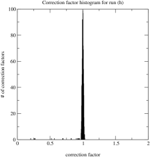
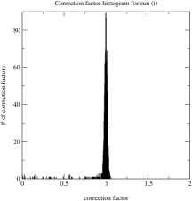
Figure 1: Correction factors for run $(h)$ (left panel) and $(i)$ (right panel).

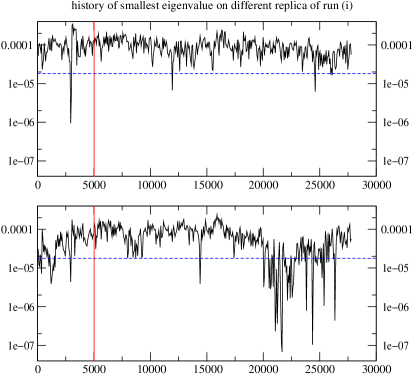
Figure 2: Histories of the smallest eigenvalue at $\beta=4.64$, $\kappa=0.197$ for two independent lattices. The upper figure shows the typical case when the smallest eigenvalue stays most of the time above $\epsilon$ shown by the dashed line. The lower figure is the history with exceptionally small eigenvalues. The measurement of physical quantities was started at the vertical line.

As has been described in subsection 2.1 a fourth polynomial $P^{(4)}_{n_{4}}$ can be used to extrapolate to infinite polynomial order therefore avoiding the need for several simulations with different orders of the second polynomial $P_{n_{2}}^{(2)}$. In our runs the evaluation of the reweighting factors was done in the way described in detail in Campos:GLUINO. Few smallest eigenvalues $\tilde{\lambda}^{2}$ of the squared hermitean fermion matrix $\tilde{Q}^{2}$, typically four, were explicitly determined and the corresponding correction factors were exactly taken into account. In the subspace orthogonal to the corresponding eigenvectors a stochastic estimate based on four Gaussian random vectors was taken. (Note that in the limit of infinite statistics a stochastic estimate always gives a correct result independently of the number of random vectors, no systematic error is introduced.)

As stated before, most of our results were obtained with second polynomials $P_{n_{2}}^{(2)}$ which gave already a good approximation of the fermionic measure. In this case the inclusion of the correction factors had nearly no influence on the final determinations since they were very close to one. Going to smaller quark masses the smallest eigenvalue starts to fluctuate more, and it is therefore no longer reasonable to try to use a second polynomial that is good enough for all cases. Such large fluctuations appeared in runs $(h)$ and $(i)$. The histograms of reweighting factors are illustrated by figure 1. It turned out that, as expected, the inclusion of the correction factors had the nice effect of reducing error bars. This is especially noticeable for fermionic quantities and in particular the pion mass which is highly correlated to the smallest eigenvalue.

Nevertheless, even in these cases the effect of reweighting was so small that the individual estimates with correction factors agreed within error bars with those without correction factors. As a whole, however, a minor systematic increase in the masses could be seen. Both histograms in figure 1 have a tail towards small values which are due to eigenvalues that could have been further suppressed by a better second polynomial. As the figure shows, this tail is more important in run $(i)$ than in run $(h)$. A closer look at the smallest eigenvalue histories in run $(i)$ reveals that the tail near zero was produced by one of the four independent parallel lattices when the smallest eigenvalue stayed for some time below the lower limit of the approximation interval $\epsilon$ (see figure 2).

Configurations with small eigenvalues $\tilde{\lambda}^{2}$ are interesting because exceptionally small values could indicate crossing of real eigenvalues of the Wilson-Dirac matrix $Q$ to the negative axis. This could give a negative sign for the determinant of a single quark flavour. We systematically analyzed in all our runs configurations with small $\tilde{\lambda}^{2}$ searching for this effect. In the present study we found, for the first time in a QCD simulation with TSMB, configurations with real negative eigenvalues of the Wilson-Dirac matrix. This happened namely in one run, run $(i)$. The (three) configurations are however statistically insignificant, since the corresponding reweighting factors are extremely small: $2.7\cdot 10^{-2},\;8.2\cdot 10^{-4}$ and $3.0\cdot 10^{-4}$. Statistically they represent less than 0.03 configurations in a sample with a total statistical weight of about 1600.

3.2.3 Results for autocorrelations

The analysis of the runs specified in table 2 gives the results for physical quantities collected in table 3. The integrated autocorrelations, where they could be determined, are given in table 4.

Table 3: Results of runs specified in table 2 for different physical quantities defined in the text. The values given in lattice units can be transformed to physical units by canceling the lattice spacing $a$ with the help of the results for $r_{0}/a$ and using $r_{0}=2.53\,{\rm GeV}^{-1}$.

run	$r_{0}/a$	$af_{\pi}$	$am_{\pi}$	$am_{\rho}$	$m_{\pi}/m_{\rho}$	$M_{r}$	$\mu_{r}$
$(a)$	1.885(30)	0.3738(50)	1.2089(36)	1.2982(32)	0.9312(17)	5.19(20)	0.498(12)
$(b)$	1.715(20)	0.4321(23)	1.0428(41)	1.1805(38)	0.8834(14)	3.20(10)	0.305(6)
$(c)$	1.616(110)	0.4171(47)	0.7886(40)	1.0251(48)	0.7693(32)	1.61(24)	0.148(11)
$(d)$	1.903(159)	0.4199(75)	0.753(11)	0.999(12)	0.752(11)	2.05(40)	0.155(13)
$(e)$	1.697(46)	0.4191(20)	0.7151(20)	0.9941(19)	0.7187(16)	1.473(88)	0.1229(41)
$(f)$	1.739(33)	0.3658(34)	0.5825(34)	0.9089(47)	0.6431(33)	1.026(51)	0.0811(30)
$(g)$	1.772(41)	0.3791(39)	0.5695(38)	0.9116(33)	0.6256(31)	1.018(61)	0.0770(32)
$(h)$	1.765(37)	0.3668(54)	0.5088(51)	0.8983(35)	0.5675(42)	0.806(50)	0.0596(27)
$(i)$	1.812(46)	0.3575(48)	0.4333(48)	0.8616(80)	0.5002(60)	0.616(45)	0.0429(21)
$(j)$	1.756(128)	0.3377(48)	0.4205(54)	0.859(12)	0.4894(65)	0.545(47)	0.0363(38)

The quoted errors of autocorrelations were estimated in different ways. For the determination of the autocorrelation of the pion mass we apply the blocking method explained in section 3.2.1. In general, one has to say that in some cases our statistics is only marginal for a precise determination of the integrated autocorrelations. In some cases (run $(a)$, $(j)$) we are not able to quote a reliable result for the autocorrelation of the pion mass.

In the high statistics runs with small quark masses $(e)$, $(f)$, $(g)$, $(h)$ and $(i)$ we had four independent parallel update sequences which could be used for a crude estimate of the errors. In addition, whenever the runs were long enough, we used binning with increasing bin lengths for the error estimates.

In general, integrated autocorrelations of the average plaquette are longest. Those for the smallest eigenvalue are comparable but sometimes by a factor 2-3 shorter. The important case of $\tau_{int}^{m_{\pi}}$ is the most favorable among the quantities we have considered: it is by a factor 2 to 10 shorter than $\tau_{int}^{plaq}$. Our experience was that the best values for $\tau_{int}^{m_{\pi}}$ could be achieved in runs where the lower limit of the approximation interval $\epsilon$ was at least by a factor of 2-3 smaller than the typical smallest eigenvalue of $\tilde{Q}^{2}$ and the multi-boson fields were relatively often updated by global quasi heatbath.

Using the values given in table 4 one can extract, for instance, the behaviour of $\tau_{int}^{plaq}$ as a function of the dimensionless quark mass parameter $M_{r}$. Since, according to table 3, the different runs are at slightly different values of $r_{0}/a$ one can correct the points with an assumed power $z_{a}=2$ to a common value, say, $r_{0}/a=1.8$. The resulting behaviour is shown by figure 3 (left panel) where a two-parameter fit $cM_{r}^{z}$ is also shown. The best fit is at $c=7.92(68)$ ($10^{6}$ MVMs), $z=-2.02(10)$ with a $\chi^{2}$ per number of degrees of freedom of $\chi^{2}/{\rm d.o.f.}=1.8$. (The result for $z$ remains the same if the common value of $r_{0}/a$ is changed in the interval $1.6\leq r_{0}/a\leq 2.0$.)

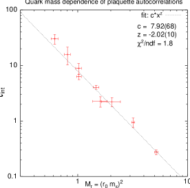
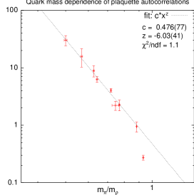
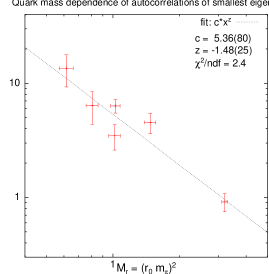
Figure 3: Left panel. Power fit of the plaquette autocorrelation given in units of $10^{6}\cdot{\rm MVM}$ as a function of the dimensionless quark mass parameter $M_{r}$. The best fit of the form $cM_{r}^{z}$ is at $c=7.92(68),\;z=-2.02(10)$. Middle panel. The same as a function of $m_{\pi}/m_{\rho}$. In this case the last point is omitted from the fit. The best fit of the form $c(m_{\pi}/m_{\rho})^{z}$ is at $c=0.476(77),\;z=-6.03(41)$. Right panel. Power fit of autocorrelation for the smallest eigenvalue of $\tilde{Q}^{2}$ given in units of $10^{6}\cdot{\rm MVM}$ as a function of the dimensionless quark mass parameter $M_{r}$. The best fit of the form $cM_{r}^{z}$ is at $c=5.36(80),\;z=-1.48(25)$.

Table 4: Integrated autocorrelations in update cycles obtained from runs specified by table 2. In the second column $C_{cycle}$ gives the number of kMVM’s ($10^{3}{\rm MVM}$’s) per update cycle. The suffix $min$, $plaq$, $\pi 8$ and $m_{\pi}$ refer to the minimal eigenvalue of $\tilde{Q}^{2}$, the average plaquette, the pion correlator at distance $d=8$ and the pion mass, respectively.

run	$C_{cycle}$	$\tau_{int}^{min}$	$\tau_{int}^{plaq}$	$\tau_{int}^{\pi 8}$	$\tau_{int}^{m_{\pi}}$
$(a)$	1.49		200(20)
$(b)$	2.45	340(60)	350(50)	152(20)	140(20)
$(c)$	4.35		420(80)		150(20)
$(d)$	5.05	$\simeq$ 310	490(90)		170(90)
$(e)$	7.34	550(110)	490(40)	274(41)	207(33)
$(f)$	7.31	810(110)	800(90)	367(110)	187(63)
$(g)$	10.5	320(80)	820(180)	466(62)	188(13)
$(h)$	16.2	380(120)	940(330)	370(88)	186(40)
$(i)$	20.4	670(210)	1500(300)	283(67)	153(54)
$(j)$	17.4	$\simeq$ 390	$\simeq$ 1050

The alternative parametrization in (2) suggests a power fit as a function of $m_{\pi}/m_{\rho}$. A good fit can only be obtained in this case if the last point with the largest quark mass is omitted (see figure 3, middle panel). The best fit parameters are in this case $c=0.476(77),\;z=-6.03(41)$ with $\chi^{2}/{\rm d.o.f.}=1.1$. The obtained power agrees very well with $z_{\pi\rho}=6$ in (2) given by the CP-PACS, JLQCD Collaboration although the latter value was obtained in a range of substantially larger quark masses on large lattices.

The data on the integrated autocorrelation of the smallest eigenvalues $\tau_{int}^{min}$ typically have larger errors. A fit of the form $cM_{r}^{z}$ is shown in figure 3 (right panel) where $c=5.36(80),\;z=-1.48(25)$ with $\chi^{2}/{\rm d.o.f}=2.4$. A fit to the integrated autocorrelation of the pion mass $\tau_{int}^{m_{\pi}}$ gives similar parameters: $c=1.99(16),\;z=-1.47(16)$ with $\chi^{2}/{\rm d.o.f}=1.7$. This shows that for $\tau_{int}^{min}$ and $\tau_{int}^{m_{\pi}}$ the quark mass dependence is described by $z_{\pi}\simeq 3$ which is, of course, more favorable than $z_{\pi}\simeq 4$ for $\tau_{int}^{plaq}$.

Concerning the quality of fits one has to remark that the different points belong to individually different optimizations of the polynomial parameters which have not necessarily the same quality. This implies an additional fluctuation beyond statistics. In view of this the $\chi^{2}$ per number of degrees of freedom values are reasonably good.

4 Eigenvalue spectra

The eigenvalue spectrum of the Wilson-Dirac matrix is interesting both physically and from the point of view of simulation algorithms. From the physical point of view the low-lying eigenvalues are expected to dominate the hadron correlators Ivanenko:LOWEIGEN; Neff:LOWEIGEN and carry information about the topological content of the background gauge field DeGrand:LOWEIGEN; Kovacs:LOWEIGEN; Horsley:LOWEIGEN. Although, as already stressed, in the present work we consider rather coarse lattices, given the importance of the question, it is interesting to see the effect of the determinant of light quarks on the qualitative properties of the eigenvalue spectrum. From the algorithmic point of view the knowledge of low-lying eigenvalues is crucial for the optimization of polynomial approximations. Finally, since we plan to perform simulations with an odd number of flavors Farchioni:QQQ, we have to consider the possibility of negative (real) eigenvalues of the non-hermitean quark matrix $Q$, which would imply a negative determinant for a single quark flavour. For $N_{f}=2$ the square of the determinant is relevant therefore the sign does not matter but the absence (or statistical insignificance) of negative eigenvalues at very small quark masses would strongly support the assumption that for the heavier strange quark there will be no problem with the determinant sign.

In order to study the low-lying spectrum of the eigenvalues we used two methods: for the eigenvalues of the hermitean fermion matrix with small absolute value the one by Kalkreuther and Simma Kalkreuter:SIMMA and for the small eigenvalues of the non-hermitean matrix the Arnoldi method Lehoucq:ARPACK; Maschho:PARPACK. The determination of the eigenvalues of the hermitean matrix is in general much faster. However, the spectrum of the non-hermitean fermion matrix contains more informations. First of all, the eigenvalues of $Q$ depend trivially on the valence hopping parameter $\kappa_{val}$ because

$$Q=1-\kappa_{val}D\ .$$ (44)

This is not true for $\tilde{Q}$. Moreover, because of the symmetries

$$Q^{\dagger}=\gamma_{5}Q\gamma_{5}\ ,\hskip 40.00006ptODO=-D\ ,$$ (45)

where $O_{xy}=(-1)^{(x1+x2+x3+x4)}\delta_{xy}$, the spectrum of $D$ is invariant under complex conjugation and sign change. As a consequence, it is sufficient to compute the low-lying spectrum of $Q$ at an arbitrary value $\kappa_{val}=\bar{\kappa}_{val}$. Other $\kappa_{val}$ are easily obtained by a shift. The value of $\bar{\kappa}_{val}$ is chosen such that it gives the best compromise of computation time and precision.

It turned out that the application of the Arnoldi algorithm is more efficient on the even-odd preconditioned matrix $\bar{Q}$ than on $Q$ itself. The analytic relation between the eigenvalues of $\bar{Q}$ and $Q$ can be used to transform the result back to $Q$. Indeed if $Q$ is written in the form

$$Q=1-\kappa\,\left(\begin{array}[]{c c}0&D_{eo}\\ D_{oe}&0\end{array}\right)$$ (46)

then $\bar{Q}$ is given by

$$\bar{Q}=1-\kappa^{2}\,\left(\begin{array}[]{c c}0&0\\ 0&D_{oe}D_{eo}\end{array}\right)\ .$$ (47)

If $v=(v_{e},v_{o})$ is an eigenvector of $Q$ with eigenvalues $\lambda$ then it satisfies

$$(\lambda v_{e},\lambda v_{o})=(v_{e}-\kappa D_{eo}v_{o},v_{o}-\kappa D_{oe}v_{e})$$ (48)

and hence

$$(1-\kappa^{2}D_{oe}D_{eo})v_{o}=v_{o}-(1-\lambda)^{2}v_{o}=\lambda(2-\lambda)v_{o}\ .$$ (49)

As a result, the eigenvalues of $\bar{Q}$ are either 1 (in the even subspace) or they satisfy

$$\bar{\lambda}=\lambda(2-\lambda)\ .$$ (50)

Because of the symmetries mentioned above, the solutions of (50) will give precisely all the eigenvalues of the matrix $Q$. This relation also gives a possibility to perform a non-trivial check of the Arnoldi code. (In addition, we also compared the algorithm with a direct computation of all the eigenvalues on a small $4^{4}$ lattice by means of a NAG library routine.) All checks confirmed the high precision given as an output by the ARPACK code, which was, in our cases, always better than $10^{-4}$ (relative precision).

4.1 Small eigenvalues

As a first task we computed the low-lying eigenvalues from sample sets of 10 configurations for runs in decreasing order of quark masses, namely those labeled with $(a)$ and $(c)$-$(j)$ in table 2. In order to have a better access to the most interesting regions of the spectrum we analyzed each configuration from two different points of view. For each configuration we first determined the 150 eigenvalues of the preconditioned Wilson-Dirac matrix ($\bar{Q}$) with smallest modulus and then the 50 eigenvalues of the non-preconditioned one ($Q$) with smallest real part.

Both computations were performed at an auxiliary value of $\kappa_{val}=0.170$, where the Arnoldi algorithm performed better. By using the analytical relations (44) and (50) we transformed the eigenvalues to those of $Q$ at the $\kappa$ value of the dynamical updates ($\kappa\equiv\kappa_{sea}$). The results are plotted in figure 4. The dashed vertical line shows the limit for the computation of the eigenvalues with smallest real part: only the part of the spectrum to the left of this line is known. In a similar way, by computing the eigenvalues with smallest modulus, we have access to the portion of the spectrum inside the dashed circle. The circle is deformed and not centered at the origin because it has been transformed together with the eigenvalues by using (50). In summary, the spectrum is not known in those points of the complex plane which are both to the right of the vertical line and outside the circle.

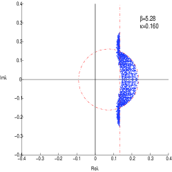
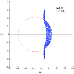
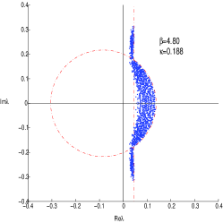
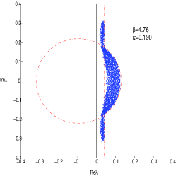
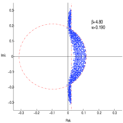
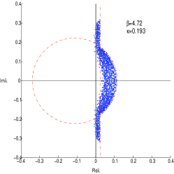
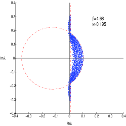
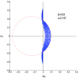
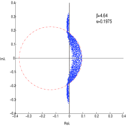
Figure 4: Low-lying eigenvalues from a set of ${\cal O}(10)$ configurations for runs $(a)$, $(c)$ to $(j)$.

Since the sequence from $(a)$ to $(j)$ corresponds to decreasing quark masses it is not a surprise that the eigenvalues have an increasing tendency to go to the left in the complex plane. At the same time they are pushed away from zero as an effect of including the fermionic determinant in the path integral measure. At very small quark masses a pronounced hole near zero is developing. For the continuum Dirac operator the spectrum is on a vertical line with some gap near zero. On our coarse lattices there is an additional horizontal spread of the eigenvalues and the picture is strongly deformed.

The size of the holes produced by the determinant is very important if we have in mind the possibility of computing observables at a partially quenched $\kappa_{val}$ higher than $\kappa_{sea}$ used in the update. The distance between the origin and the smallest real eigenvalue determines how much smaller masses (larger $\kappa_{val}$) one can reach by partial quenching before encountering exceptional configurations. This question can be answered by studying configurations with exceptionally small eigenvalues. Of course, the reweighting factors discussed in section 3.2.2 have to be taken into account in this analysis because they suppress such configurations to a large extent.

4.2 Negative eigenvalues

One of the purposes of the analysis of the eigenvalues was to determine whether there is a statistically significant presence of configurations with negative determinant. As already said, the sign of the determinant is easy to determine from the low-lying spectrum since it is negative if an odd number of real negative eigenvalues occurs. In fact, non-real eigenvalues always appear in conjugate pairs. In the randomly chosen set of configurations reported above we did not find a single real negative eigenvalue. However, a set of ${\cal O}(10)$ configurations is a rather small subsample.

Additional information on the presence or absence of negative eigenvalues in our samples is given by the distribution of reweighting factors. Crossing of eigenvalues to negative real axis implies small reweighting factors corresponding to very small eigenvalues of $\tilde{Q}^{2}$ below the lower bound of the interval $[\epsilon,\lambda]$. The calculation of reweighting factors, which was carried out on every configuration in the selected subsamples, is much cheaper than the analysis of small eigenvalues of the non-hermitean matrix $Q$. As we discussed in section 3.2.2, the distribution of reweighting factors is strongly peaked near one in all runs, except for runs $(h)$ and $(i)$ which have high statistics at very small quark masses (see figure 1). In these cases there are a few configurations with reweighting factors close to zero. In order to see whether the small reweighting factors (and the corresponding small eigenvalues of $\tilde{Q}^{2}$) are associated to negative eigenvalues or not, we concentrated on configurations with particularly small eigenvalues of $\tilde{Q}^{2}$.

Note that there is no simple analytical relation between the lowest eigenvalues of the hermitean and the non-hermitean matrix but it is reasonable to expect that small eigenvalues occur together. This expectation was confirmed in all cases we investigated. An interesting observation was that very small eigenvalues of the hermitean matrix seem to be usually associated to small real eigenvalues of the non-hermitean one. This is compatible with the fact that real eigenvalues do not need to be double degenerate and therefore they can afford to approach closer to the origin than a complex conjugate pair.

In figure 5 two significant examples are reported. The first set of configurations in the figure corresponds to a moderately small quark mass (run $(h)$) and the second to a very small quark mass (run $(i)$). In both cases we selected the configurations with smallest eigenvalues of $\tilde{Q}^{2}$. Even in this way we could not find a single real negative eigenvalue for the first run $(h)$. In the second case we found three configurations with negative eigenvalues. The (in total) four negative eigenvalues are visible in the detail in the right panel of figure 5. As stated before these configurations are statistically insignificant.

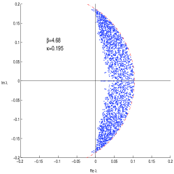
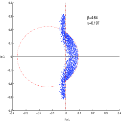
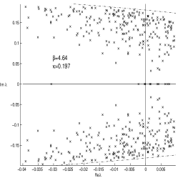
Figure 5: Low-lying eigenvalues for a set of 10 configurations with exceptionally small eigenvalues, at $\beta=4.68$ and $\kappa=0.195$ (left panel), $\beta=4.64$ and $\kappa=0.197$ (middle panel), detail (right panel).

Some comments are in order. We have collected strong evidence that the presence of configurations with negative determinant is irrelevant at this stage. Of course it is not yet possible to tell how this picture will evolve on larger volumes and closer to the continuum limit. It will be necessary to keep monitoring the low part of the spectrum as we did here. Since, to that purpose, we only need to know a very small part of the spectrum, there is no reason to think that this task should become too difficult on large volumes.

As a last remark we should stress that we performed this analysis of the sign for very small quark masses. Even if (partially quenched) Chiral Perturbation Theory is valid for any combination of the quark masses, it is probably not worth having an unpaired sea quark with a mass much smaller than the strange quark. Therefore, provided that the picture will not dramatically change on larger lattices, for all physical circumstances it seems very unlikely that the determinant sign could become a problem.

4.3 Flow of eigenvalues

By using the algorithm of Kalkreuther and Simma Kalkreuter:SIMMA we also explored the flow of the spectrum $\{\tilde{\lambda}\}$ of the hermitean matrix $\tilde{Q}$ for a wide range of valence $\kappa$ values, going from zero bare quark mass to a large negative one. This is interesting in view of simulations of dynamical fermions with Neuberger’s operator Neuberger:OPE, where the inverse square root of $\tilde{Q}^{2}$ with negative valence mass has to be taken. The optimal valence mass should be chosen in a region where $\tilde{Q}$ has no eigenvalues extremely close to zero, namely where a “gap” is opening up in the spectrum near $\tilde{\lambda}=0$. The results for two typical configurations are plotted in figure 6. For large negative masses we observed many sign changes and the eigenvalue with smallest absolute value is always close to zero. It seems that for dynamical Wilson fermions on our coarse lattice there is no gap-opening near $\tilde{\lambda}=0$.

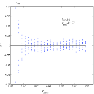
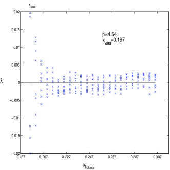
Figure 6: Computation of 8 eigenvalues closest to zero of the hermitean Wilson-Dirac matrix for two configurations from the run at $\beta=4.64$ and $\kappa=0.197$.

A possible application of the eigenvalue flow is to monitor the number of negative eigenvalues at $\kappa=\kappa_{sea}$ Edwards:FLOW; Campos:GLUINO. This is substantially cheaper than the analysis of the spectrum of non-hermitean matrix $Q$ by the Arnoldi method. For instance, observing the eigenvalue flow one can easily exclude the absence of negative eigenvalues if there is no crossing of zero in the flow below $\kappa_{sea}$ – which is the typical case. A more detailed (and more expensive) analysis can be restricted to the seldom case when a crossing occurs.

5 Discussion

Our runs on $8^{3}\cdot 16$ lattices with lattice spacing of about $a\simeq 0.27\,{\rm fm}$ for $N_{f}=2$ degenerate quarks display the dependence of simulation costs on the quark mass. Assuming the parametrization in (1) with $z_{L}=5$ and $z_{a}=2$, from the integrated autocorrelation of the average plaquette we obtain

$$z_{\pi}\simeq 4\ ,\hskip 30.00005ptF\simeq 0.8\cdot 10^{9}\,{\rm flop}\ .$$ (51)

The power for the quark mass dependence $z_{\pi}$ comes out smaller than $z_{\pi\rho}=6$ in the form (2) quoted by the CP-PACS, JLQCD Collaboration Ukawa:BERLIN but if we omit the point with largest quark mass and perform a fit with the parametrization (2) we also obtain $z_{\pi\rho}\simeq 6$ (see figure 3).

As shown by figure 3 (left panel), our data on the integrated autocorrelation of the average plaquette are well fitted by $z_{\pi}=4$ in the whole range $0.6\leq M_{r}\leq 6$ which approximately corresponds to $\frac{1}{5}m_{s}\leq m_{ud}\leq 2m_{s}$. The data on the integrated autocorrelation of the smallest eigenvalue of the squared hermitean fermion matrix show an even weaker power $z_{\pi}\simeq 3$ but there the errors are larger and the fit is less convincing (see right panel in figure 3). The pion mass has the shortest autocorrelation; this also shows a power $z_{\pi}\simeq 3$. $z_{\pi}=4$ corresponds to a behaviour proportional to the inverse square of the quark mass. Qualitatively speaking, according to table 4, one inverse quark mass power is due to the increase of the condition number of the fermion matrix and another inverse power comes from the increase of the autocorrelation in numbers of update cycles. Note that because of $(r_{0}m_{\pi})^{2}\propto(r_{0}m_{q})$ the case of $z_{\pi}=4,\;z_{a}=2$ corresponds to a situation when the scale parameter $r_{0}$ cancels in the cost formula (1).

The overall factor $F$ given in (51) is such that for our second smallest quark mass $M_{r}\simeq 0.6$ (run $(i)$) the cost in floating point operations comes out to be $C\simeq 2.3\cdot 10^{14}$. As table 4 shows, considering instead of the integrated autocorrelation of the average plaquette the one of the pion mass, the result is $C\simeq 0.4\cdot 10^{14}$. The parameters in (2) give the same number. The other estimates for Wilson-type quarks in Lippert:BERLIN and Wittig:BERLIN in this point are: $C_{L}\simeq 0.2\cdot 10^{14}$ and $C_{W}\simeq 1.1\cdot 10^{14}$, respectively. Taking into account that the numbers $C_{U,L,W}$ have been obtained under rather different circumstances concerning simulation algorithm, autocorrelations considered, quark mass range, lattice size and even lattice action there is a surprisingly good order of magnitude agreement.

It is remarkable that in a rather broad range of quark masses $\frac{1}{5}m_{s}\leq m_{ud}\leq m_{s}$ (leaving out the point at $m_{ud}\simeq 2m_{s}$) two fits with $z_{\pi}=4$ and $z_{\pi\rho}=6$ work equally well (figure 3). This implies in this range of quark masses a peculiar dependence of $m_{\pi}/m_{\rho}$ on $M_{r}$ (see figure 7, where the relation between the two different quark mass parameters $\mu_{r}$ and $M_{r}$ is also shown). However, the two parametrizations in (1) and (2) cannot be both correct in the vicinity of zero quark mass because there the two powers have to be equal: $z_{\pi\rho}=z_{\pi}$. Saying it differently, the extrapolations of the two fits below $m_{ud}=\frac{1}{5}m_{s}$ are different. The fit with $z_{\pi\rho}=6$ gives a more dramatic slowing down near zero quark mass than the one with $z_{\pi}=4$. The real asymptotics near $m_{ud}=0$ could be disentangled by going to still smaller quark masses. With TSMB there is no serious obstacle for doing this – except for the increase in necessary computer time.

The value of the lattice spacing in this paper is chosen rather large in order to limit the computational costs for these tests. Our aim was to concentrate on the quark mass dependence in the range of light quarks. Further studies will be needed for investigating the cost as a function of the lattice spacing (in particular, the value of the exponent $z_{a}$) for smaller values of $a$. In this respect the experience of the DESY-Münster-Roma Collaboration in the supersymmetric Yang-Mills theory at much smaller lattice spacings ($a\simeq 0.06{\rm fm}$) Campos:GLUINO; Farchioni:SUSYWTI shows already that TSMB has a decent behaviour also closer to the continuum limit.

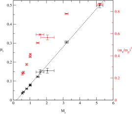
Figure 7: The dependence of $(m_{\pi}/m_{\rho})^{2}$ on $M_{r}$ according to table 3 (right values). The values of $\mu_{r}$ are also shown (left) together with a linear fit (dashed line).

Besides the quark mass dependence of simulation costs, the other interesting question we investigated in this paper is the distribution of the small eigenvalues of the fermion matrix and, in particular, the existence of negative fermion determinants of a single quark flavour. Our data show that the effect of the fermion determinant is rather explicit because of the strong suppression of the eigenvalue density near zero (see figures 4-5). The statistical weight of configurations with negative determinant is negligible even at our smallest quark masses. In fact after an extensive analysis we only found three configurations with negative determinant at our second smallest quark mass $M_{r}\simeq 0.6$ (run $(i)$) and none of them at other quark masses. Taking into account the small reweighting factors of the configurations with negative determinant, their relative statistical weight is ${\cal O}(10^{-5})$.

It is clear that it would be important to check the volume dependence of our results, both for simulation costs and small eigenvalues, on larger lattices and closer to the continuum limit. We plan to do this in the future.

  

Acknowledgement

The computations were performed on the APEmille systems installed at NIC Zeuthen, the Cray T3E systems at NIC Jülich and the PC clusters at DESY Hamburg. We thank H. Simma for help with APEmille programming and optimization, M. Lüscher for providing his SSE code, H. Wittig for useful discussions on various topics, T. Kovacs and W. Schroers for sharing with us their experience about the computation of eigenvalues, and R. Peetz for careful reading of the manuscript.