Abstract

We discuss the salient features of Zolotarev optimal rational approximation for the inverse square root function, in particular, for its applications in lattice QCD with overlap Dirac quark. The theoretical error bound for the matrix-vector multiplication $H_{w}(H_{w}^{2})^{-1/2}Y$ is derived. We check that the error bound is always satisfied amply, for any QCD gauge configurations we have tested. An empirical formula for the error bound is determined, together with its numerical values ( by evaluating elliptic functions ) listed in Table 2 as well as plotted in Figure 3. Our results suggest that with Zolotarev approximation to $(H_{w}^{2})^{-1/2}$, one can practically preserve the exact chiral symmetry of the overlap Dirac operator to very high precision, for any gauge configurations on a finite lattice.

PACS numbers: 11.15.Ha, 11.30.Rd, 12.38.Gc, 02.60.Pn, 02.60-x

Keywords : Rational Approximation, Zolotarev optimal rational approximation, Error bound, Overlap Dirac operator, Lattice QCD

1 Introduction

In lattice QCD with overlap Dirac quarks [1, 2], one encounters the challenging problem of taking the inverse square root of a positive definite Hermitian matrix, which stems from the overlap Dirac operator for massless fermion

$$D=m_{0}a^{-1}\left(1+\gamma_{5}{H_{w}\over\sqrt{H_{w}^{2}}}\right)\ ,$$ (1)

where $H_{w}$ denotes the Hermitian Wilson-Dirac operator with a negative parameter $-m_{0}$,

$$H_{w}=\gamma_{5}D_{w}=\gamma_{5}(-m_{0}+\gamma_{\mu}t_{\mu}+W)\ ,$$ (2)

$\gamma_{\mu}t_{\mu}$ the naive fermion operator, and $W$ the Wilson term. It is well-known that (1) is the simplest and the most elegant realization of chiral symmetry on a finite lattice [3]

$$D\gamma_{5}+\gamma_{5}D=am_{0}^{-1}D\gamma_{5}D\ ,$$ (3)

and it also fulfils all basic requirements ( i.e., doublers-free, $\gamma_{5}$-hermiticity, exponentially-local, and correct continuum behavior ) for a decent lattice Dirac operator. However, in practice, how to compute physical quantities in lattice QCD with overlap Dirac operator (1) is still a challenging problem, due to the inverse square root of $H_{w}^{2}$ in (1), which cannot be evaluated analytically in a closed form, nor numerically via diagonalization since the memory requirement exceeds the physical memory of the present generation of computers. Thus, at this stage, it is necessary to replace $(H_{w}^{2})^{-1/2}$ with a good approximation, in any lattice QCD calculations with overlap Dirac quark. The relevant question is what is the optimal rational approximation $r_{n}(x)$ ( of degree $n$ ) for the inverse square root function $x^{-1/2},x\in[1,b]$, in view of the convergence of a rational approximation can attain

$$\max_{1\leq x\leq b}|1-\sqrt{x}r_{n}(x)|=c_{1}e^{-c_{2}n}\ ,\hskip 17.07164ptc_{1},\ c_{2}>0\ ,$$ (4)

which is much faster than that of any polynomial approximation. It turns out that the optimal solution has been obtained by Zolotarev [4] more than 100 years ago. A detailed discussion of Zolotarev’s result can be found in Akhiezer’s two books [5, 6]. Unfortunately, Zolotarev’s optimal rational approximation has been overlooked by the numerical algebra community until recent years.

A comparative study of Zolotarev’s approximation versus other schemes for computing the product of the matrix sign function $H_{w}(H_{w}^{2})^{-1/2}$ with a vector $Y$, has been reported in Ref. [8].

Recently, we have used Zolotarev optimal rational approximation to compute overlap Dirac quark propagator in the quenched approximation [9]. The parameters of the pseudoscalar meson mass formula to one-loop order in chiral perturbation theory are determined, and from which the light quark masses $m_{u,d}$ and $m_{s}$ can be extracted [10] with the experimental inputs of pion and kaon masses, and the pion decay constant.

Nevertheless, in Refs. [8, 9], the underlying principles and salient features of Zolotarev optimal rational approximation have not been addressed. Also, in Refs. [7, 8, 9], only one option (70) of the two possible choices [(29) and (70)] of Zolotarev’s rational polynomials has been exploited, however, these two options are complementary to each other, and in some cases it is more effective to use (29) than (70), in computing $(H_{w}^{2})^{-1/2}$ times a column vector $Y$, as discussed in Section 5.

In this paper, we discuss the salient features of Zolotarev optimal rational approximation, in particular, for its application in lattice QCD with overlap Dirac operator. We start with the basic principles of rational approximation, and show that Zolotarev’s rational polynomial is indeed the optimal rational approximation for the inverse square root function. Then we examine how well the Zolotarev optimal rational approximation (48) for the overlap Dirac operator can preserve the exact chiral symmetry (3) on a finite lattice. For the overlap Dirac operator, (3) is equivalent to

$$\left({H_{w}\over\sqrt{H_{w}^{2}}}\right)^{2}=1\ .$$ (5)

Thus the question is how much the exact relation (5) is violated if one replaces $(H_{w}^{2})^{-1/2}$ with Zolotarev’s optimal rational polynomial $r^{(n)}_{Z}(H_{w}^{2})$. The chiral symmetry breaking can be measured in terms of the deviation

$$\Delta_{Z}=\max_{\forall\ Y\neq 0}\left|{Y^{\dagger}\{H_{w}r^{(n)}_{Z}(H_{w}^{2})\}^{2}Y\over Y^{\dagger}Y}-1\right|\ .$$ (6)

It turns out that the deviation (6) has a theoretical upper bound (62), which is a function of $n$ ( the degree of the rational polynomial ), and $b=\lambda_{max}^{2}/\lambda_{min}^{2}$, where $\lambda_{max}^{2}$ and $\lambda_{min}^{2}$ denote the maximum and the minimum of the eigenvalues of $H_{w}^{2}$. Thus, for any given gauge configuration, one can use the theoretical upper bound to determine what values of $n$ and $b$ ( i.e., how many low-lying eigenmodes of $H_{w}^{2}$ should be projected out ) are required to attain one’s desired accuracy in preserving the chiral symmetry of the overlap Dirac operator. In practice, one has no difficulties to achieve $\Delta_{Z}<10^{-12}$ for any gauge configurations on a finite lattice.

The outline of this paper is as follows. In Sections 2-4, we review the basic principles of rational approximation, and show that Zolotarev’s rational polynomial is indeed the optimal rational approximation for the inverse square root function. In Section 5, we discuss the Zolotarev approximation for $(H_{w}^{2})^{-1/2}$ in the overlap Dirac operator, and derive the theoretical error bound for the matrix-vector multiplication $H_{w}(H_{w}^{2})^{-1/2}Y$ ( $Y$ : any nonzero column vector ), which is the most essential operation in computing the propagator of overlap Dirac quark by nested conjugate gradient. We check that the theoretical error bound is always satisfied amply, for any QCD gauge configurations we have tested. Then the numerical values of the theoretical error bound are computed, and listed in Table 2, as well as plotted in Figure 3. An empirical formula for the error bound is determined from the numerical data. In Section 6, we conclude with some remarks.

2 de la Vallée-Poussin’s theorem

First we consider the following problem. Given any two positive and continuous functions $f(x)$ and $g(x)$ for $x\in[1,b]$, the problem is to find the irreducible rational polynomial of degree $n$ with positive real coefficients,

$$r(x)={p(x)\over q(x)}={p_{n}x^{n}+p_{n-1}x^{n-1}+\cdots+p_{0}\over q_{n}x^{n}+q_{n-1}x^{n-1}+\cdots+q_{0}}\ ,$$ (7)

such that the deviation of $g(x)r(x)$ from $f(x)$ is the minimum. Here the deviation is defined as the maximum of $|f(x)-g(x)r(x)|$ for the entire interval $[1,b]$, i.e.,

$$d(r)=\max_{x\in[1,b]}|f(x)-g(x)r(x)|\ .$$ (8)

Now if there exists $r(x)$ such that the difference

$$\delta(x)=f(x)-g(x)r(x)$$ (9)

changes sign alternatively $2n+2$ times within the interval $[1,b]$, and attains its maxima and minima, say,

$$\delta(x)=\delta_{1},-\delta_{2},\cdots,+\delta_{2n+1},-\delta_{2n+2}\hskip 17.07164pt(\delta_{i}>0)$$ (10)

at consecutive points,

$$x_{1}<x_{2}<\cdots<x_{2n+2}\ ,$$ (11)

then it can be shown that

$$d(r)\geq\min\{\delta_{1},\delta_{2},\cdots,\delta_{2n+2}\}\equiv d_{min}$$ (12)

for all irreducible rational polynomial $r(x)$ as defined by (7). This can be asserted as follows.

The strategy is to assume the contrary is true, and then show that it leads to contradiction. Suppose there exists an irreducible rational polynomial $R(x)$ of degree $n$, such that $d(R)<d_{min}$. Then

$$D(x) \equiv g(x)R(x)-g(x)r(x)$$ (13)

$$= f(x)-g(x)r(x)-[f(x)-g(x)R(x)]$$

$$= \delta(x)-\Delta(x)$$

is a continuous function, and it also changes sign alternatively at least $2n+2$ times in the interval $[1,b]$, since $|\Delta(x)|\leq d(R)<d_{min}$. Thus $D(x)$ has at least $2n+1$ zeros in the interval $(1,b)$. On the other hand,

$$D(x)=g(x)[R(x)-r(x)]\equiv g(x){u(x)\over v(x)}$$ (14)

where $u(x)$ and $v(x)$ are polynomials of degree $2n$. Therefore $D(x)$ cannot have more than $2n$ zeros, i.e., a contradiction. This completes the proof of de la Vallée-Poussin’s theorem.

In general, de la Vallée-Poussin’s theorem[5] asserts that if there exists an irreducible rational polynomial of the form

$$r^{(n,m)}(x)={p_{n}x^{n}+p_{n-1}x^{n-1}+\cdots+p_{0}\over q_{m}x^{m}+q_{m-1}x^{m-1}+\cdots+q_{0}}\ ,\ (m\geq n,\ p_{i},q_{i}>0)$$ (15)

such that $\delta(x)=f(x)-g(x)r^{(n,m)}(x)$ has $n+m+2$ alternate change of sign in the interval $[1,b]$, and attains its maxima and minima, say,

$$\delta(x)=\delta_{1},-\delta_{2},\cdots,(-1)^{n+m+1}\delta_{n+m+2}\hskip 17.07164pt(\delta_{i}>0)$$

at consecutive points,

$$x_{1}<x_{2}<\cdots<x_{n+m+2}\ ,$$

then

$$d(r)\geq\min\{\delta_{1},\delta_{2},\cdots,\delta_{n+m+2}\}\equiv d_{min}$$

for all irreducible rational polynomial $r^{(n,m)}(x)$.

In the next section, we show that there exists an optimal $r_{Z}(x)$ such that $d(r_{Z})$ is minimum, i.e., Zolotarev’s solution [4].

3 Zolotarev’s optimal rational approximation

First, we recall some well-known properties of Jacobian elliptic functions [6]. The Jacobian elliptic function $\mbox{sn}(u;\kappa)=\eta$ is defined by the elliptic integral

$$u(\eta)=\int_{0}^{\eta}{dt\over\sqrt{(1-t^{2})(1-\kappa^{2}t^{2})}}\ .$$ (16)

It is a meromorphic function of $u$ and $\kappa$, which is defined over $\mbox{CC}^{2}$. For $\eta=1$, (16) becomes

$$u(1)\equiv K=\int_{0}^{1}{dt\over\sqrt{(1-t^{2})(1-\kappa^{2}t^{2})}}\ ,$$ (17)

the complete elliptic integral of the first kind with modulus $\kappa$.

The important feature of $\mbox{sn}(u;\kappa)$ is that it is periodic in both real and imaginary parts of $u$,

$$\mbox{sn}(u+4K;\kappa)=\mbox{sn}(u;\kappa)$$ (18)

$$\mbox{sn}(u+2iK^{\prime};\kappa)=\mbox{sn}(u;\kappa)$$ (19)

where $K^{\prime}$ is complete elliptic integral of the first kind with modulus $\kappa^{\prime}=\sqrt{1-\kappa^{2}}$

Now if we define

$$x(u;\kappa)\equiv\mbox{sn}^{2}(u;\kappa)\ ,$$ (20)

then $x$ has periods $2K$ and $2iK^{\prime}$, since $\mbox{sn}(u+2K;\kappa)=-\mbox{sn}(u;\kappa)$.

The crucial formula for Zolotarev’s optimal rational approximation is the second principal $n$-th degree transformation of Jacobian elliptic function [6]. In terms of $x$ (20), it reads

$$\sqrt{x\left({u\over M};\lambda\right)}=\sqrt{x(u;\kappa)}{1\over M}\prod_{l=1}^{n}{1+x(u;\kappa)/c_{2l}\over 1+x(u;\kappa)/c_{2l-1}}$$ (21)

where

$$\lambda = \prod_{l=1}^{2n+1}{\Theta^{2}\left({2lK^{\prime}\over 2n+1};\kappa^{\prime}\right)\over\Theta^{2}\left({(2l-1)K^{\prime}\over 2n+1};\kappa^{\prime}\right)}\ ,$$ (22)

$$M = \prod_{l=1}^{n}{\mbox{sn}^{2}\left({(2l-1)K^{\prime}\over 2n+1};\kappa^{\prime}\right)\over\mbox{sn}^{2}\left({2lK^{\prime}\over 2n+1};\kappa^{\prime}\right)}\ ,$$ (23)

$$c_{l} = {\mbox{sn}^{2}({lK^{\prime}\over 2n+1};\kappa^{\prime})\over 1-\mbox{sn}^{2}({lK^{\prime}\over 2n+1};\kappa^{\prime})},$$ (24)

and $\Theta$ denotes the elliptic theta function. Note that $x(u/M;\lambda)$ has periods $2L=2K/M$ and $2iL^{\prime}=2iK^{\prime}/[(2n+1)M]$,

$$x\left({u+2K\over M};\lambda\right) = x\left({u\over M};\lambda\right)$$ (25)

$$x\left({u\over M}+{2iK^{\prime}\over(2n+1)M};\lambda\right) = x\left({u\over M};\lambda\right)\ .$$ (26)

Now restricting $u=K+iv$, we have

$$x(u;\kappa)=\mbox{sn}^{2}(u;\kappa)={1-\mbox{sn}^{2}(iv;\kappa)\over 1-\kappa^{2}\mbox{sn}^{2}(iv;\kappa)}={1\over 1-{\kappa^{\prime}}^{2}\mbox{sn}^{2}(v;\kappa^{\prime})}\ ,$$ (27)

where the identity

$$\mbox{sn}^{2}(iv;\kappa)=-{\mbox{sn}^{2}(v;\kappa^{\prime})\over 1-\mbox{sn}^{2}(v;\kappa^{\prime})}$$ (28)

has been used. Equation (27) implies that $x$ increases from $1$ to $1/\kappa^{2}$ as $v$ increases from $0$ to $K^{\prime}$, since $\mbox{sn}(0;\kappa^{\prime})=0$, and $\mbox{sn}(K^{\prime};\kappa^{\prime})=1$, from the definition (16).

Now consider

$$r_{Z}(x)={2\lambda\over 1+\lambda}{1\over M}\prod_{l=1}^{n}{1+x/c_{2l}\over 1+x/c_{2l-1}}$$ (29)

as a rational approximation to $1/\sqrt{x}$. Then the deviation can be obtained from

$$\delta_{Z}(x)=1-\sqrt{x}r_{Z}(x)=1-{2\lambda\over 1+\lambda}\mbox{sn}\left({K+iv\over M};\lambda\right)$$ (30)

where (21) has been used. Using identity (27) with substitutions $\kappa\leftarrow\lambda$ and $u\leftarrow(K+iv)/M$, then (30) becomes

$$\delta_{Z}(x)=1-{2\lambda\over 1+\lambda}{1\over\sqrt{1-{\lambda^{\prime}}^{2}\mbox{sn}^{2}\left({v\over M};\lambda^{\prime}\right)}}\ ,$$ (31)

where $\lambda^{\prime}=\sqrt{1-\lambda^{2}}$. As $v$ changes from $0$ to $K^{\prime}$, $v/M$ changes from $0$ to $K^{\prime}/M=(2n+1)L^{\prime}$. This implies that $\mbox{sn}^{2}\left(v/M;\lambda^{\prime}\right)$ attains its minima and maxima alternatively as $0,1,\cdots,0,1$ at $v/M=0,L^{\prime},\cdots,2nL^{\prime},(2n+1)L^{\prime}$. Correspondingly, $\delta_{Z}(x)$ reaches its maxima and minima alternatively as

$${1-\lambda\over 1+\lambda},-{1-\lambda\over 1+\lambda},\cdots,{1-\lambda\over 1+\lambda},-{1-\lambda\over 1+\lambda}$$ (32)

at $v/M=0,L^{\prime},\cdots,2nL^{\prime},(2n+1)L^{\prime}$, which correspond to $2n+2$ successive $x\in[1,1/\kappa^{2}]$,

$$1,{1\over 1-\kappa^{\prime 2}\mbox{sn}^{2}\left({K^{\prime}\over 2n+1};\kappa^{\prime}\right)},\cdots,{1\over 1-\kappa^{\prime 2}\mbox{sn}^{2}\left({2nK^{\prime}\over 2n+1};\kappa^{\prime}\right)},{1\over\kappa^{2}}\ .$$ (33)

That is,

$$x_{i}={1\over 1-\kappa^{\prime 2}\mbox{sn}^{2}\left({(i-1)K^{\prime}\over 2n+1};\kappa^{\prime}\right)}\ ,\ i=1,\cdots,2n+2\ .$$ (34)

From (32), we conclude that

$$d(r_{Z})={1-\lambda\over 1+\lambda}=d_{min}\ ,$$ (35)

and Zolotarev’s solution (29) is the optimal rational approximation for the inverse square root function, according to de la Vallée-Poussin’s theorem.

At this point, it is instructive to plot $\delta_{Z}(x)=1-\sqrt{x}r_{Z}(x)$ explicitly, and to see how it attains its maxima and minima alternatively. This is shown in Fig. 1 for $n=6$ and $b=\kappa^{-2}=1000$. Note that there are exactly $2n+2=14$ alternate change of sign in $[1,1000]$, with maxima and minima at

$$x = 1,\ 1.145,\ 1.664,\ 2.858,\ 5.415,\ 10.80,\ 22.05,\ 45.34,$$

$$92.59,\ 184.7,\ 349.9,\ 600.9,\ 873.3,\ 1000.$$

In Fig. 2, we plot the positions $x_{i}$ (34) of the maxima and minima of $\delta_{Z}(x)=1-\sqrt{x}r_{Z}(x)$ for $n=20$ and $b=\kappa^{-2}=6000$. Note that the distribution of $x_{i}$ as shown in Fig. 2 is quite generic for any values of $n$ and $b$. The maxima and minima near both ends ( $x_{1}=1$ and $x_{2n+2}=b$ ) are densely packed even in the logarithm scale, while those at the central region seem to be evenly distributed in log scale ( i.e., exponentially in the linear scale ).

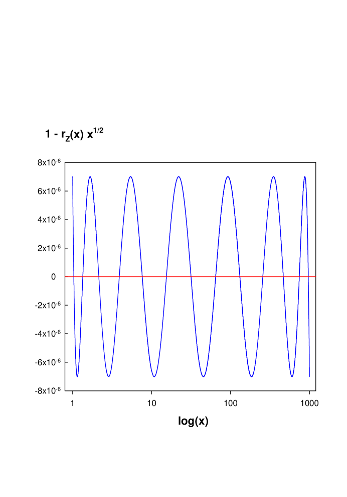
Figure 1: The difference $1-\sqrt{x}r_{Z}(x)$ of Zolotarev optimal rational approximation (29) with $n=6$ and $b=\kappa^{-2}=1000$. Note that there are exactly $2n+2=14$ alternate change of sign in $[1,1000]$, and the maxima and minima have exactly the same magnitude.

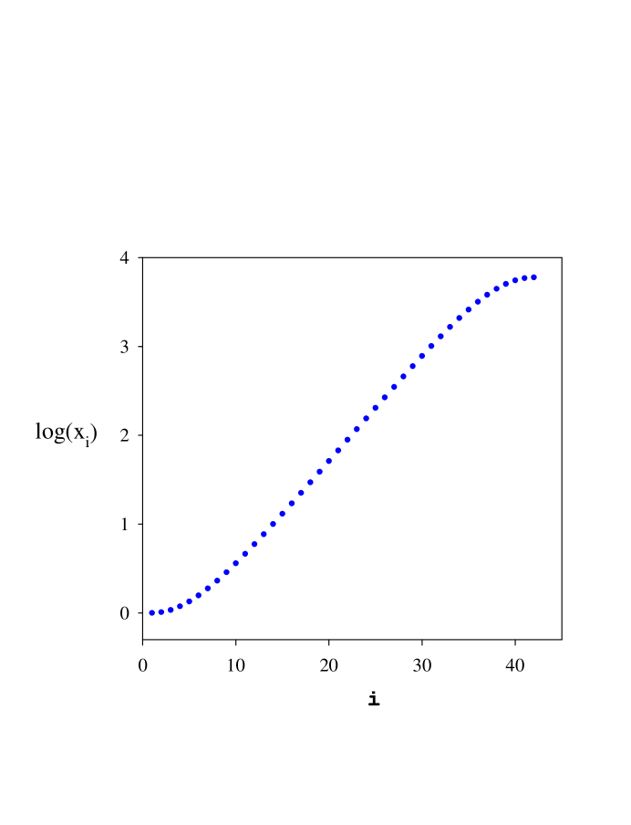
Figure 2: The positions $x_{i}$ (34) of the maxima and minima of $1-\sqrt{x}r_{Z}(x)$ for $n=20$ and $b=\kappa^{-2}=6000$.

4 Chebycheff’s theorem

Even though Zolotarev’s rational approximation is optimal among all irreducible rational polynomials of degree $n$, with $\delta(x)=f(x)-g(x)r(x)$ having $2n+2$ alternate change of sign in $[1,b]$, one may still ask whether there exists an optimal irreducible rational polynomial of the same degree but its $\delta(x)$ has smaller number of alternate change of sign in $[1,b]$. Such a possibility is ruled out by Chebycheff’s theorem, which can be shown as follows.

Again, our strategy is to assume the contrary is true, and then show that it leads to contradiction. Suppose there exists an optimal rational polynomial $R(x)=P(x)/Q(x)$ of degree $n$ with deviation $d(R)=d_{min}$, but its $\Delta(x)\equiv f(x)-g(x)R(x)$ only has $m=2n+1$ alternate change of sign in $[1,b]$. Now assume $\Delta(x)$ attains its maxima and minima, say,

$$\Delta(x)=\Delta_{1},-\Delta_{2},+\Delta_{3},\cdots,+\Delta_{m}\hskip 17.07164pt(\Delta_{i}>0)$$ (36)

at consecutive points

$$1=x_{1}<x_{2}<\cdots<x_{m}=b\ .$$ (37)

Then the interval $[1,b]$ can be divided into $m$ subintervals,

$$[1,\xi_{1}],[\xi_{1},\xi_{2}],\cdots,[\xi_{m-1},b]\ ,\hskip 17.07164ptx_{i}<\xi_{i}<x_{i+1}$$ (38)

such that the following two inequalities can be satisfied alternatively,

$$-d_{min}+\epsilon< \Delta(x) \leq d_{min}\ ,\hskip 11.38109ptx\in[\xi_{2i-2},\xi_{2i-1}],\ i=1,\cdots,n+1$$ (39)

$$-d_{min}\leq \Delta(x) <d_{min}-\epsilon\ ,\hskip 11.38109ptx\in[\xi_{2i-1},\xi_{2i}],\ i=1,\cdots,n$$ (40)

where $\epsilon$ is a positive number which is much less than $d_{min}$, and the notations $\xi_{0}=1$ and $\xi_{m}=b$ have been used.

Next consider the following polynomial of degree $2n=m-1$

$$S(x)=(x-\xi_{1})(x-\xi_{2})\cdots(x-\xi_{m-1})$$ (41)

which has sign change at $\xi_{i},i=1,\cdots,m-1$. Using the fact that $P(x)$ and $Q(x)$ have no common factor, one can find polynomials $U(x)$ and $V(x)$ of degree $n$, with positive real coefficients, such that

$$S(x)=Q(x)U(x)-P(x)V(x)\ .$$ (42)

Now consider the following irreducible rational polynomial of degree $n$

$$W(x)={P(x)+\alpha U(x)\over Q(x)+\alpha V(x)}$$ (43)

where $\alpha$ is a positive real parameter. Then, the difference

$$f(x)-g(x)W(x) = f(x)-g(x)R(x)+g(x)R(x)-g(x)W(x)$$ (44)

$$= \Delta(x)-\alpha g(x){S(x)\over Q(x)[Q(x)+\alpha V(x)]}\ ,$$

is a function of $\alpha$ which can be chosen to be some tiny positive numbers such that the magnitude of the second term on the r.h.s. of (44) is much less than $d_{min}-\epsilon$ for all $x\in[1,b]$, i.e.,

$$0<\alpha g(x){|S(x)|\over Q(x)[Q(x)+\alpha V(x)]}\leq\mu\ll d_{min}-\epsilon\ .$$ (45)

Since $\Delta(x)$ and $S(x)$ both have $m=2n+1$ alternate change of sign in $[1,b]$, and the magnitude of the second term on r.h.s. of (44) is very small comparing to $d_{min}-\epsilon$, it follows that $f(x)-g(x)W(x)$ also has $m=2n+1$ alternate change of sign in $[1,b]$.

Then, using (39), (41), (44) and (45), we obtain

$$-d_{min}+\epsilon-\mu<f(x)-g(x)W(x)\leq d_{min}-\mu\ ,$$ (46)

for $x\in[\xi_{2i-2},\xi_{2i-1}],i=1,\cdots,n+1$. Similarly, we have

$$-d_{min}+\mu\leq f(x)-g(x)W(x)\leq d_{min}-\epsilon+\mu\ ,$$ (47)

for $x\in[\xi_{2i-1},\xi_{2i}],i=1,\cdots,n$ . Thus we obtain that $d(W)=d_{min}-\mu<d_{min}$, a contradiction to our assumption that $R(x)$ is the optimal one. This completes the proof of Chebycheff’s theorem.

In general, Chebycheff’s theorem asserts that the optimal irreducible rational polynomial of the form (15) must satisfy the criterion that the difference $\delta(x)=f(x)-g(x)r^{(n,m)}(x)$ has $n+m+2$ alternate change of sign in the interval $[1,b]$.

5 Zolotarev approximation for the overlap

In this section, we first derive the theoretical error bound for the the matrix-vector multiplication $H_{w}(H_{w}^{2})^{-1/2}Y$ ( $Y$ : any nonzero column vector ) with Zolotarev approximation for $(H_{w}^{2})^{-1/2}$. Then the numerical values of the error bound are computed, and listed in Table 1, as well as plotted in Figure 3. An empirical formula for the error bound is determined from the data.

5.1 Error bound for $H_{w}(H_{w}^{2})^{-1/2}_{Z}Y$

To use Zolotarev approximation for the $(H_{w}^{2})^{-1/2}$ in the overlap Dirac operator (1), one needs to rescale $H_{w}$ to $h_{w}=H_{w}/\lambda_{min}$ such that the eigenvalues of $h_{w}^{2}$ fall in the interval $[1,b]$, where $b=(\lambda_{max}/\lambda_{min})^{2}$. Explicitly

$${1\over\sqrt{H_{w}^{2}}}\simeq{d_{0}\over\lambda_{min}}\prod_{l=1}^{n}{h_{w}^{2}+c_{2l}\over h_{w}^{2}+c_{2l-1}}={1\over\lambda_{min}}(h_{w}^{2}+c_{2n})\sum_{l=1}^{n}{b_{l}\over h_{w}^{2}+c_{2l-1}}\equiv(H_{w}^{2})^{-1/2}_{Z}$$ (48)

where

$$d_{0} = {2\lambda\over 1+\lambda}\prod_{l=1}^{n}{1+c_{2l-1}\over 1+c_{2l}}$$ (49)

$$b_{l} = d_{0}{\prod_{i=1}^{n-1}(c_{2i}-c_{2l-1})\over\prod_{i=1,i\neq l}^{n}(c_{2i-1}-c_{2l-1})}\ .$$ (50)

First, we consider the multiplication of $H_{w}(H_{w}^{2})^{-1/2}$ to a nonzero column vector $Y$

$$H_{w}\left({1\over\sqrt{H_{w}^{2}}}\right)Y\simeq h_{w}(h_{w}^{2}+c_{2n})\sum_{l=1}^{n}{b_{l}\over h_{w}^{2}+c_{2l-1}}Y=h_{w}(h_{w}^{2}+c_{2n})\sum_{l=1}^{n}b_{l}Z_{l}$$ (51)

where the last summation can be evaluated by invoking a conjugate gradient process to the linear systems

$$(h_{w}^{2}+c_{2l-1})Z_{l}=Y,\hskip 11.38109ptl=1,\cdots,n\ .$$ (52)

In order to improve the accuracy of the rational approximation as well as to reduce the number of iterations in the conjugate gradient loop, it is advantageous to narrow the interval $[1,b]$ by projecting out the largest and some low-lying eigenmodes of $H_{w}^{2}$. Denoting these eigenmodes by

$$H_{w}u_{j}=\lambda_{j}u_{j},\hskip 11.38109ptj=1,\cdots,k,$$ (53)

then we project the linear systems (52) to the complement of the vector space spanned by these eigenmodes

$$(h_{w}^{2}+c_{2l-1})\bar{Z_{l}}=\bar{Y}\equiv(1-\sum_{j=1}^{k}u_{j}u_{j}^{\dagger})Y\ ,\hskip 11.38109ptl=1,\cdots,n\ .$$ (54)

In the set of projected eigenvalues of $H_{w}^{2}$, $\{\lambda_{j}^{2},j=1,\cdots,k\}$, we use $\lambda_{max}^{2}$ and $\lambda_{min}^{2}$ to denote the least upper bound and the greatest lower bound for the eigenvalues of $\bar{H}_{w}^{2}$, where

$$\bar{H}_{w}=H_{w}-\sum_{j=1}^{k}\lambda_{j}u_{j}u_{j}^{\dagger}\ .$$

Then the eigenvalues of

$$h_{w}^{2}=\bar{H}_{w}^{2}/\lambda_{min}^{2}$$

fall into the interval $(1,b)$, $b=(\lambda_{max}/\lambda_{min})^{2}$.

Now the matrix-vector multiplication (51) can be expressed in terms of the projected eigenmodes (53) plus the solution obtained from the conjugate gradient loop (54) in the complementary vector space, i.e.,

$$H_{w}{1\over\sqrt{H_{w}^{2}}}Y\simeq{1\over\lambda_{min}}\bar{H}_{w}(h_{w}^{2}+c_{2n})\sum_{l=1}^{n}b_{l}\bar{Z}_{l}+\sum_{j=1}^{k}{\lambda_{j}\over\sqrt{\lambda_{j}^{2}}}u_{j}u_{j}^{\dagger}Y\equiv S$$ (55)

Then the error of $S$ can be measured in terms of

$$\sigma={|S^{\dagger}S-Y^{\dagger}Y|\over Y^{\dagger}Y}\ ,$$ (56)

which is zero if (55) is exact. Now assuming the errors due to the conjugate gradient and the projected eigenmodes are negligible compared with that due to the Zolotarev approximation of $(h_{w}^{2})^{-1/2}$, then we can derive the theoretical upper bound of $\sigma$ as follows.

First, we rewrite $S$ (55) as

$$S=\sum_{j=1}^{k}{\lambda_{j}\over\sqrt{\lambda_{j}^{2}}}u_{j}u_{j}^{\dagger}Y+\sum_{j=k+1}^{N}\mbox{sign}(\lambda_{j})\sqrt{x_{j}}r_{Z}(x_{j})u_{j}u_{j}^{\dagger}Y\ ,\hskip 11.38109ptx_{j}\equiv\left({\lambda_{j}\over\lambda_{min}}\right)^{2}$$ (57)

where $\lambda_{j},u_{j},j=k+1,\cdots,N$ denote the eigenvalues and eigenfunctions of $\bar{H}_{w}$. Then it is straightforward to derive

$$S^{\dagger}S-Y^{\dagger}Y=Y^{\dagger}\left(\sum_{j=k+1}^{N}[(\sqrt{x_{j}}r_{Z}(x_{j}))^{2}-1]u_{j}u_{j}^{\dagger}\right)Y\ ,$$ (58)

where the orthonormality ( $u_{i}^{\dagger}u_{j}=\delta_{ij}$ ) has been used. Thus it follows that

$$|S^{\dagger}S-Y^{\dagger}Y| \leq \max_{k+1\leq j\leq N}|(\sqrt{x_{j}}r_{Z}(x_{j}))^{2}-1|\ Y^{\dagger}\left(\sum_{l=k+1}^{N}u_{l}u_{l}^{\dagger}\right)Y$$ (59)

$$< \max_{k+1\leq j\leq N}|(\sqrt{x_{j}}r_{Z}(x_{j}))^{2}-1|\ Y^{\dagger}Y$$

where the inequality ( due to the completeness relation $\sum_{l=1}^{N}u_{l}u_{l}^{\dagger}=\mbox{1I}$ )

$$Y^{\dagger}\left(\sum_{l=k+1}^{N}u_{l}u_{l}^{\dagger}\right)Y<Y^{\dagger}Y\ ,\hskip 11.38109pt(k>0)$$

has been used. Then the theoretical upper bound of (56) is

$$\sigma<\max_{k+1\leq j\leq N}|(\sqrt{x_{j}}r_{Z}(x_{j}))^{2}-1|\simeq 2\max_{k+1\leq j\leq N}|\sqrt{x_{j}}r_{Z}(x_{j})-1|\ .$$ (60)

Thus $\sigma$ is less than two times of the maximum of $|1-\sqrt{x_{j}}r_{Z}(x_{j})|$ for all eigenvalues of $h_{w}^{2}$. It follows that $\sigma$ must be less than two times of the maximum of $|1-\sqrt{x}r_{Z}(x)|$ for all $x\in[1,b]$, i.e.,

$$\sigma={|S^{\dagger}S-Y^{\dagger}Y|\over Y^{\dagger}Y}<{2(1-\lambda)\over 1+\lambda}\equiv 2d_{Z}(n,b)\ ,$$ (61)

where $\lambda$ is defined in (22). The inequality (61) is one of the main results of this paper.

A remarkable feature of (61) is that it holds for any nonzero column vector $Y$. Then one immediately sees that the deviation (6) which measures the chiral symmetry breaking due to Zolotarev approximation also has the same theoretical upper bound,

$$\Delta_{Z}<2d_{Z}(n,b)\ .$$ (62)

Thus $2d_{Z}(n,b)$ not only serves as the theoretical error bound for the matrix-vector multiplication $H_{w}(H_{w}^{2})^{-1/2}_{Z}Y$, but also provides the upper bound for the chiral symmetry breaking due to Zolotarev approximation. Note that $d_{Z}(n,b)$ does not depend on the lattice size explicitly. Therefore, by choosing the proper values of $n$ and $b$ ( i.e., by projecting the high and low-lying eigenmodes of $H_{w}^{2}$ ), one can practically preserve the exact chiral symmetry of the overlap Dirac operator to very high precision, for any gauge configurations on a finite lattice.

Moreover, for any gauge configuration, it is unlikely that any of the eigenvalues of $h_{w}^{2}$ would coincide with one of those $2n+2$ positions with maximum deviation (34), thus one usually obtains a $\sigma$ much smaller than the theoretical error bound $2d_{Z}(n,b)$.

In Table 1, we list the values of $\sigma$ (56) for several gauge configurations on three different lattices respectively, along with the theoretical error bound $2d_{Z}(n,b)$. It is clear that $\sigma$ is always much smaller than the theoretical error bound. Note that for each configuration, we only show the largest $\sigma$ among a set of several hundred $\sigma$ values, each is computed with a different $Y$ at every iteration of the outer CG loop. The average value of $\sigma$ is usually less than $1/5$ of the largest one listed in Table 1. Details of our computation are described in [9]. Here we have set the stopping criterion for the inner and outer conjugate gradient loops at $\epsilon=10^{-11}$, and the error of the projected eigenmodes around $10^{-13}$. It is remarkable that $\sigma$ turns out to be much less than $\epsilon$, in contrast to one’s naive expectation. In other words, even if the precision of the overlap Dirac quark propagator is only up to $10^{-11}$, its exact chiral symmetry can attain $\Delta_{Z}<10^{-12}$.

lattice size	$\beta$	$\lambda_{min}$	$\lambda_{max}$	$b$	$n$	$\sigma$	$2d_{Z}(n,b)$
$16^{3}\times 32$	$6.0$	$0.1731$	$6.258$	1307.00	$12$	$6.0\times 10^{-12}$	$1.4\times 10^{-10}$
$16^{3}\times 32$	$6.0$	$0.1943$	$6.260$	1038.01	$12$	$7.0\times 10^{-12}$	$7.5\times 10^{-11}$
$16^{3}\times 32$	$6.0$	$0.1767$	$6.261$	1255.49	$12$	$8.0\times 10^{-12}$	$1.2\times 10^{-10}$
$16^{3}\times 32$	$6.0$	$0.1955$	$6.260$	1025.31	$12$	$5.0\times 10^{-12}$	$7.2\times 10^{-11}$
$12^{3}\times 24$	$5.8$	$0.1176$	$6.210$	2788.49	$16$	$7.0\times 10^{-14}$	$4.8\times 10^{-13}$
$12^{3}\times 24$	$5.8$	$0.1285$	$6.211$	2336.24	$16$	$6.6\times 10^{-14}$	$3.2\times 10^{-13}$
$12^{3}\times 24$	$5.8$	$0.0988$	$6.206$	3945.57	$16$	$2.0\times 10^{-13}$	$1.3\times 10^{-12}$
$12^{3}\times 24$	$5.8$	$0.1415$	$6.213$	1927.92	$16$	$5.5\times 10^{-14}$	$1.6\times 10^{-13}$
$10^{3}\times 24$	$5.8$	$0.1242$	$6.214$	2503.22	$16$	$1.6\times 10^{-13}$	$3.4\times 10^{-13}$
$10^{3}\times 24$	$5.8$	$0.1381$	$6.209$	2021.42	$16$	$6.1\times 10^{-14}$	$2.2\times 10^{-13}$
$10^{3}\times 24$	$5.8$	$0.1376$	$6.204$	2032.86	$16$	$5.5\times 10^{-14}$	$2.6\times 10^{-13}$
$10^{3}\times 24$	$5.8$	$0.1181$	$6.204$	2759.59	$16$	$4.4\times 10^{-14}$	$5.0\times 10^{-13}$

Table 1: The error $\sigma$ (56) of the matrix-vector multiplication $H_{w}(H_{w}^{2})^{-1/2}_{Z}Y$, for several gauge configurations on three different lattices. Evidently, each $\sigma$ is quite smaller than the corresponding theoretical error bound $2d_{Z}(n,b)=2(1-\lambda)/(1+\lambda)$.

5.2 An empirical formula for the error bound

In Table 2, we list the values of $d_{Z}(n,b)=(1-\lambda)/(1+\lambda)$ of Zolotarev optimal rational appproximation (29), for $n\simeq 10-20$ and $b\simeq 10-10^{6}$. We can use Table 2 to determine how many Zolotarev terms ( $n$ ) is needed in order to attain one’s desired accuracy, after the highest and the low-lying eigenmodes are projected out and $b=(\lambda_{max}/\lambda_{min})^{2}$ has been obtained. Conversely, for a fixed number of Zolotarev terms, say $n$, one can use Table 2 to determine what ranges of high and low-lying eigenmodes of $H_{w}^{2}$ should be projected in order to attain one’s desired accuracy.

$b$	$n$
	10	12	14	16	18	20
$10$	$4.8\times 10^{-18}$	$1.9\times 10^{-21}$	$7.2\times 10^{-25}$	$2.8\times 10^{-28}$	$1.1\times 10^{-31}$	$4.1\times 10^{-35}$
$50$	$1.3\times 10^{-13}$	$3.5\times 10^{-16}$	$9.5\times 10^{-19}$	$2.6\times 10^{-21}$	$6.9\times 10^{-24}$	$1.9\times 10^{-26}$
$100$	$2.5\times 10^{-12}$	$1.2\times 10^{-14}$	$5.5\times 10^{-17}$	$2.6\times 10^{-19}$	$1.2\times 10^{-21}$	$5.8\times 10^{-24}$
$500$	$3.8\times 10^{-10}$	$4.8\times 10^{-12}$	$5.9\times 10^{-14}$	$7.3\times 10^{-16}$	$9.0\times 10^{-18}$	$1.1\times 10^{-19}$
$1000$	$2.0\times 10^{-9}$	$3.4\times 10^{-11}$	$5.8\times 10^{-13}$	$9.8\times 10^{-15}$	$1.7\times 10^{-16}$	$2.8\times 10^{-18}$
$2000$	$8.4\times 10^{-9}$	$1.9\times 10^{-10}$	$4.2\times 10^{-12}$	$9.3\times 10^{-14}$	$2.1\times 10^{-15}$	$4.6\times 10^{-17}$
$3000$	$1.8\times 10^{-8}$	$4.6\times 10^{-10}$	$1.2\times 10^{-11}$	$3.0\times 10^{-13}$	$7.7\times 10^{-15}$	$2.0\times 10^{-16}$
$4000$	$2.9\times 10^{-8}$	$8.3\times 10^{-10}$	$2.3\times 10^{-11}$	$6.6\times 10^{-13}$	$1.9\times 10^{-14}$	$5.3\times 10^{-16}$
$5000$	$4.3\times 10^{-8}$	$1.3\times 10^{-9}$	$3.9\times 10^{-11}$	$1.2\times 10^{-12}$	$3.6\times 10^{-14}$	$1.1\times 10^{-15}$
$6000$	$5.7\times 10^{-8}$	$1.8\times 10^{-9}$	$5.8\times 10^{-11}$	$1.9\times 10^{-12}$	$6.0\times 10^{-14}$	$1.9\times 10^{-15}$
$7000$	$7.2\times 10^{-8}$	$2.4\times 10^{-9}$	$8.1\times 10^{-11}$	$2.7\times 10^{-12}$	$9.1\times 10^{-14}$	$3.1\times 10^{-15}$
$8000$	$8.9\times 10^{-8}$	$3.1\times 10^{-9}$	$1.1\times 10^{-10}$	$3.7\times 10^{-12}$	$1.3\times 10^{-13}$	$4.5\times 10^{-15}$
$9000$	$1.1\times 10^{-7}$	$3.8\times 10^{-9}$	$1.4\times 10^{-10}$	$4.9\times 10^{-12}$	$1.8\times 10^{-13}$	$6.4\times 10^{-15}$
$1\times 10^{4}$	$1.2\times 10^{-7}$	$4.6\times 10^{-9}$	$1.7\times 10^{-10}$	$6.3\times 10^{-12}$	$2.3\times 10^{-13}$	$8.6\times 10^{-15}$
$5\times 10^{4}$	$9.5\times 10^{-7}$	$5.2\times 10^{-8}$	$2.9\times 10^{-9}$	$1.6\times 10^{-10}$	$8.6\times 10^{-12}$	$4.7\times 10^{-13}$
$1\times 10^{5}$	$2.0\times 10^{-6}$	$1.3\times 10^{-7}$	$8.0\times 10^{-9}$	$5.0\times 10^{-10}$	$3.2\times 10^{-11}$	$2.0\times 10^{-12}$
$5\times 10^{5}$	$8.7\times 10^{-6}$	$7.3\times 10^{-7}$	$6.1\times 10^{-8}$	$5.0\times 10^{-9}$	$4.2\times 10^{-10}$	$3.5\times 10^{-11}$
$1\times 10^{6}$	$1.5\times 10^{-5}$	$1.4\times 10^{-6}$	$1.3\times 10^{-7}$	$1.2\times 10^{-8}$	$1.1\times 10^{-9}$	$1.0\times 10^{-10}$

Table 2: The deviation $d_{Z}(n,b)=\max|1-\sqrt{x}r^{(n,n)}_{Z}(x)|=(1-\lambda)/(1+\lambda)$ of the Zolotarev optimal rational approximation (29), versus the upper bound $b$ of $x\in[1,b]$, and the degree $n$ of the rational polynomial.

In Fig. 3, we plot $d_{Z}(n,b)=\max|1-\sqrt{x}r^{(n,n)}_{Z}(x)|=(1-\lambda)/(1+\lambda)$ versus the degree $n$, for different values of $b$ ranging from $10^{3}-10^{6}$. For any fixed value of $b$, the error bound converges exponentially with respect to $n$, and it is well fitted by

$$e_{Z}(n,b)=A(b)\exp\{-c(b)n\}\ ,$$ (63)

as indicated by the solid lines shown in Fig. 3. The parameters $c(b)$ and $A(b)$ are determined in Figs. 4 and 5 respectively,

$$c(b) = 9.17(10)\ \mbox{ln}(b)^{-0.774(5)}$$ (64)

$$A(b) = 0.465(9)\ \mbox{ln}(b)^{0.596(9)}$$ (65)

With the empiraical formula (63), one can estimate the theoretical upper bound of $\sigma$ or $\Delta_{Z}$ more conveniently, without evaluating ellitpic functions at all.

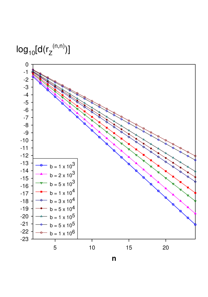
Figure 3: The error bound of Zolotarev optimal rational approximation for the inverse square root function $x^{-1/2},x\in[1,b]$, versus the degree $n$ of the rational polynomial, and for several different values of $b$ ranging from $10^{3}$ to $10^{5}$. For any fixed value of $b$, the error bound converges exponentially with respect to $n$, and is well fitted by $A(b)\exp\{-c(b)n\}$ with $c(b)=9.17(10)\mbox{ln}(b)^{-0.774(5)}$ and $A(b)=0.465(9)\mbox{ln}(b)^{0.596(9)}$.

Figure 4: Determination of the parameters of $c(b)$

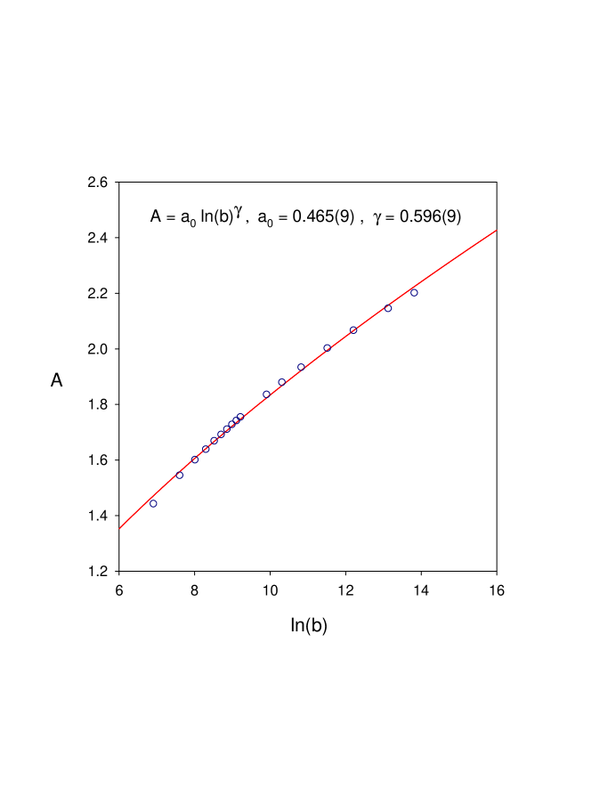
Figure 5: Determination of the parameters of $A(b)$

5.3 Zolotarev rational polynomial of the form $r^{(n-1,n)}$

At this point, if one recalls Chebycheff’s therorem for $r^{(n,m)}$, one may ask whether there exists optimal rational approximation to $x^{-1/2}$, which has the form $r^{(n-1,n)}$, with $1-\sqrt{x}r^{(n-1,n)}_{Z}(x)$ having $2n+1$ alternate change of sign in $[1,b]$. Note that in the second principal $n$-th degree transformation (21), $\mbox{sn}(x/M;\lambda)$ has periods $2K/M$ and $2iK^{\prime}/[(2n+1)M]$. Thus there must exist a similar transformation in which $\mbox{sn}(x/M;\lambda)$ has periods $2K/M$ and $2iK^{\prime}/2nM$. Explicitly, it reads

$$\sqrt{x\left({u\over m};\Lambda\right)}=\sqrt{x(u;\kappa)}{1\over m}{\prod_{l=1}^{n-1}[1+x(u;\kappa)/{C}_{2l}]\over\prod_{l=1}^{n}[1+x(u;\kappa)/{C}_{2l-1}]}$$ (66)

where

$$\Lambda = \prod_{l=1}^{2n}{\Theta^{2}\left({2lK^{\prime}\over 2n};\kappa^{\prime}\right)\over\Theta^{2}\left({(2l-1)K^{\prime}\over 2n};\kappa^{\prime}\right)}\ ,$$ (67)

$$m = {\prod_{l=1}^{n}\mbox{sn}^{2}\left({(2l-1)K^{\prime}\over 2n};\kappa^{\prime}\right)\over\prod_{l=1}^{n-1}\mbox{sn}^{2}\left({2lK^{\prime}\over 2n};\kappa^{\prime}\right)}\ ,$$ (68)

$${C}_{l} = {\mbox{sn}^{2}({lK^{\prime}\over 2n};\kappa^{\prime})\over 1-\mbox{sn}^{2}({lK^{\prime}\over 2n};\kappa^{\prime})},$$ (69)

Then the Zolotarev optimal rational polynomial of the form $r^{(n-1,n)}$ is

$$r^{(n-1,n)}_{Z}(x)={2\Lambda\over 1+\Lambda}{1\over m}{\prod_{l=1}^{n-1}(1+x/{C}_{2l})\over\prod_{l=1}^{n}(1+x/{C}_{2l-1})}$$ (70)

The difference $1-\sqrt{x}r^{(n-1,n)}_{Z}(x)$ has $2n+1$ alternate change of sign in $[1,b]$, ( $b=\kappa^{-2}$ ), and it attains its maxima and minima alternatively as

$${1-\Lambda\over 1+\Lambda},-{1-\Lambda\over 1+\Lambda},\cdots,-{1-\Lambda\over 1+\Lambda},{1-\Lambda\over 1+\Lambda}$$

at $2n+1$ successive points $x\in[1,b]$ :

$$1,{1\over 1-\kappa^{\prime 2}\mbox{sn}^{2}\left({K^{\prime}\over 2n};\kappa^{\prime}\right)},\cdots,{1\over 1-\kappa^{\prime 2}\mbox{sn}^{2}\left({(2n-1)K^{\prime}\over 2n};\kappa^{\prime}\right)},{1\over\kappa^{2}}\ .$$

Obviously, for any given $n$ and $b$, the deviation of $r^{(n-1,n)}_{Z}$ is larger than that of $r^{(n,n)}_{Z}$, i.e.,

$$d(r^{(n-1,n)}_{Z})={1-\Lambda\over 1+\Lambda}>{1-\lambda\over 1+\lambda}=d(r^{(n,n)}_{Z})\ ,$$ (71)

and for most cases,

$$d(r^{(n-1,n)}_{Z})\simeq 2.5\times d(r^{(n,n)}_{Z})$$ (72)

In Table 3, we list the deviation $d(r^{(n-1,n)}_{Z})=(1-\Lambda)/(1+\Lambda)$ of the Zolotarev optimal rational appproximation (70), versus the degree $n$, and the upper bound $b$ of $x\in[1,b]$. Comparing the corresponding entries ( with the same $b$ and $n$ ) in Table 3 and Table 2, one immediately sees that $d(r^{(n-1,n)}_{Z})\simeq 2.5\times d(r^{(n,n)}_{Z})$.

If one uses (70) to approximate the inverse square root of $H_{w}^{2}$ in the overlap Dirac operator, then one has

$${1\over\sqrt{H_{w}^{2}}}\simeq{D_{0}\over\lambda_{min}}{\prod_{l=1}^{n-1}(h_{w}^{2}+C_{2l})\over\prod_{l=1}^{n}(h_{w}^{2}+C_{2l-1})}={D_{0}\over\lambda_{min}}\sum_{l=1}^{n}{B_{l}\over h_{w}^{2}+C_{2l-1}}$$ (73)

where

$$D_{0} = {2\Lambda\over 1+\Lambda}{\prod_{l=1}^{n}(1+C_{2l-1})\over\prod_{l=1}^{n-1}(1+C_{2l})}$$ (74)

$$B_{l} = D_{0}{\prod_{i=1}^{n-1}(C_{2i}-C_{2l-1})\over\prod_{i=1,i\neq l}^{n}(C_{2i-1}-C_{2l-1})}\ .$$ (75)

Comparing (48) with (73), one immediately sees that it is more advantageous to use the former approximation than the latter, especially for computing quark propagators, since only one more matrix multiplication with $(h_{w}^{2}+c_{2n})$ after the completion of the inner CG loop would yield about $2.5$ times higher accuracy than using (73). Although we used (73) for our computations in Ref. [9], we have switched to (48) for better accuracy, in our ongoing lattice QCD computations.

$b$	$n$
	10	12	14	16	18	20
1000	$5.6\times 10^{-9}$	$9.4\times 10^{-11}$	$1.6\times 10^{-12}$	$2.7\times 10^{-14}$	$4.6\times 10^{-16}$	$7.8\times 10^{-18}$
2000	$2.2\times 10^{-8}$	$4.8\times 10^{-10}$	$1.1\times 10^{-11}$	$2.4\times 10^{-13}$	$5.3\times 10^{-15}$	$1.2\times 10^{-16}$
3000	$4.5\times 10^{-8}$	$1.1\times 10^{-9}$	$2.9\times 10^{-11}$	$7.5\times 10^{-13}$	$1.9\times 10^{-14}$	$5.0\times 10^{-16}$
4000	$7.2\times 10^{-8}$	$2.0\times 10^{-9}$	$5.7\times 10^{-11}$	$1.6\times 10^{-12}$	$4.6\times 10^{-14}$	$1.3\times 10^{-15}$
5000	$1.0\times 10^{-7}$	$3.1\times 10^{-9}$	$9.4\times 10^{-11}$	$2.8\times 10^{-12}$	$8.6\times 10^{-14}$	$2.6\times 10^{-15}$
6000	$1.3\times 10^{-7}$	$4.3\times 10^{-9}$	$1.4\times 10^{-10}$	$4.4\times 10^{-12}$	$1.4\times 10^{-13}$	$4.5\times 10^{-15}$
7000	$1.7\times 10^{-7}$	$5.7\times 10^{-9}$	$1.9\times 10^{-10}$	$6.4\times 10^{-12}$	$2.1\times 10^{-13}$	$7.2\times 10^{-15}$
8000	$2.1\times 10^{-7}$	$7.1\times 10^{-9}$	$2.5\times 10^{-10}$	$8.7\times 10^{-12}$	$3.0\times 10^{-13}$	$1.1\times 10^{-14}$
9000	$2.4\times 10^{-7}$	$8.7\times 10^{-9}$	$3.1\times 10^{-10}$	$1.1\times 10^{-11}$	$4.1\times 10^{-13}$	$1.5\times 10^{-14}$
10000	$2.8\times 10^{-7}$	$1.0\times 10^{-8}$	$3.9\times 10^{-10}$	$1.4\times 10^{-11}$	$5.3\times 10^{-13}$	$2.0\times 10^{-14}$

Table 3: The deviation $d(r^{(n-1,n)}_{Z})=\max|1-\sqrt{x}r^{(n-1,n)}_{Z}(x)|=(1-\Lambda)/(1+\Lambda)$ of the Zolotarev optimal rational approximation (70) versus the upper bound $b$ of $x\in[1,b]$, and the degree $n$ of the rational polynomial.

6 Concluding remarks

In this paper, we have discussed the basic principles underlying the rational approximation, and shown explicitly that the Zolotarev approximation is indeed the optimal rational approximation for the inverse square root function. For the overlap Dirac operator, we have derived the theoretical error bound for the matrix-vector multiplication $H_{w}(H_{w}^{2})^{-1/2}_{Z}Y$, which is equal to two times of the maximum deviation $d_{Z}(n,b)$ of the Zolotarev rational polynomial. This is also the upper bound for the chiral symmetry breaking due to Zolotarev approximation. Some numerical values of $d_{Z}(n,b)$ are listed in Table 2 as well as plotted in Figure 3. An empirical formula for $d_{Z}(n,b)$ is determined, which provides a reliable estimate of the theoretical error bound, especially for the range of parameters : $b\simeq 10^{3}-10^{4}$ and $n\simeq 10-20$. We also compare two possible forms of Zolotarev optimal rational approximation : $r_{Z}^{(n,n)}(x)$ and $r^{(n-1,n)}_{Z}(x)$, and point out that the former seems to be the better choice for computing quark propagators, since with the same computational cost, one has $d(r^{(n,n)}_{Z})\simeq 0.4\times d(r^{(n-1,n)}_{Z})$.

With Zolotarev optimal rational approximation for $(H_{w}^{2})^{-1/2}$ in the overlap Dirac operator, one has no difficulties to preserve exact chiral symmetry to very high precision ( e.g., $\Delta_{Z}<10^{-12}$ ), for any gauge configurations on a finite lattice. This feature is vital for lattice QCD to extract physical observables from the first principles. In practice, one might have difficulties to push the error $\sigma$ (56) down below $10^{-13}$, which is essentially due to the inaccuracies of the projected ( high and low-lying ) eigenmodes of $H_{w}^{2}$, rather than the Zolotarev approximation of $(H_{w}^{2})^{-1/2}$. In the future, we will try to improve the accuracy of the projected eigenmodes. In the meantime, the precision of exact chiral symmetry up to $10^{-13}$ should be sufficient for many calculations in lattice QCD with overlap Dirac quarks.

This work was supported in part by the National Science Council, ROC, under the grant number NSC90-2112-M002-021, and also in part by NCTS.

References

- [1] H. Neuberger, Phys. Lett. B 417, 141 (1998)
- [2] R. Narayanan and H. Neuberger, Nucl. Phys. B 443, 305 (1995)
- [3] P. H. Ginsparg and K. G. Wilson, Phys. Rev. D 25, 2649 (1982).
- [4] E. I. Zolotarev, “Application of elliptic functions to the questions of functions deviating least and most from zero”, Zap. Imp. Akad. Nauk. St. Petersburg, 30 (1877), no. 5; reprinted in his Collected works, Vol. 2, Izdat, Akad. Nauk SSSR, Moscow, 1932, p. 1-59.
- [5] N. I. Akhiezer, ”Theory of approximation”, Reprint of 1956 English translation. Dover, New York, 1992.
- [6] N. I. Akhiezer, ”Elements of the theory of elliptic functions”, second revised edition, Izdat. ”Nauka”, Moscow, 1970. Translations of Mathematical Monographs, 79. American Mathematical Society, Providence, R.I. 1990.
- [7] D. Ingerman, V. Druskin, L. Knizhnerman, Comm. Pure Appl. Math. 53(8), 1039 (2000).
- [8] J. van den Eshof, A. Frommer, T. Lippert, K. Schilling and H. A. van der Vorst, Comput. Phys. Commun. 146, 203 (2002)
- [9] T. W. Chiu and T. H. Hsieh, Phys. Rev. D 66, 014506 (2002)
- [10] T. W. Chiu and T. H. Hsieh, Phys. Lett. B 538, 298 (2002)