$I=2$ Pion Scattering Length with the Wilson Fermion

Abstract

The calculation of the $I=2$ pion scattering length in quenched lattice QCD is revisited. The calculation is carried out with the Wilson fermion action employing Lüscher’s finite size scaling method at $\beta=5.9$, $6.1$, and $6.3$ corresponding to the range of lattice spacing $a\simeq 0.12-0.07$ fm. We obtain in the continuum limit $a_{0}/m_{\pi}=-2.09(35)\ 1/{\rm GeV}^{2}$, which is consistent with the prediction of chiral perturbation theory $a_{0}/m_{\pi}=-2.265(51)\ 1/{\rm GeV}^{2}$.

Lattice calculations of $S$-wave scattering lengths of the two-pion system are important step to understand dynamical effects of strong interactions. There are already a number of calculations for the $I=2$ process with either Staggered [1, 2] or Wilson fermion action [1, 3]. While these calculations gave results that are in gross agreement with the prediction of chiral perturbation theory (CHPT) [4], they were made on coarse and small lattices. More importantly, the continuum extrapolation was not made. Aiming to improve on these points, we carried out a calculation of the $I=2$ $S$-wave scattering length in quenched lattice QCD. A preliminary result was reported in Ref. [5], in which some disagreement with the CHPT prediction was mentioned. In the mean time Liu et.al. carried out a similar calculation with the improved gauge and the Wilson fermion actions on anisotropic lattices [6].

We employ the standard plaquette action for gluons and the Wilson action for quarks, and explore the parameter range $m_{\pi}/m_{\rho}\sim 0.55-0.80$ for the chiral extrapolation and $a\sim 0.07-0.12$ fm for the continuum extrapolation. This is compared with the parameters of Liu et.al. which range $m_{\pi}/m_{\rho}\sim 0.7-0.9$ and $a_{s}\sim 0.2-0.4$ fm. Our calculations are made for parameters significantly closer to the chiral limit. In this short report we give the final result of our analysis.

The numbers of configurations (lattice sizes) are $187~{}(16^{3}\times 64)$, $120~{}(24^{3}\times 64)$, and $100~{}(32^{3}\times 80)$ for $\beta=5.9$, $6.1$, and $6.3$, respectively. Quark propagators are solved with the Dirichlet boundary condition in the time direction and the periodic boundary condition in the space directions. The pion mass covers the range of $450-900{\rm MeV}$. The lattice constant is estimated from the $\rho$ meson mass, which was obtained in our previous study[7], to be $a^{-1}=1.64(2),2.29(4),3.02(5)$ (GeV) at $\beta=5.9$, $6.1$, and $6.3$. Our calculations were carried out on the Fujitsu VPP500/80 supercomputer at KEK.

The energy eigenvalue of a two-pion system in a finite periodic box $L^{3}$ is shifted by the finite-size effect. Lüscher presented a relation between the energy shift $\Delta E$ and the $S$-wave scattering length $a_{0}$, given by [8]

$$-\Delta E\cdot\frac{m_{\pi}L^{2}}{4\pi^{2}}=T+C_{1}\cdot T^{2}+C_{2}\cdot T^{3}+O(T^{4})\ ,$$ (1)

where $T=a_{0}/(\pi L)$. The constants are $C_{1}=-8.9136$ and $C_{2}=62.9205$ computed from geometry of the lattice. Since $T$ has a small value, typically $\sim-10^{-2}$ in our simulation, we can safely neglect the higher order terms $O(T^{4})$.

The energy shift $\Delta E$ can be obtained from the ratio $R(t)=G(t)/D(t)$, where

$$G(t)=\langle\pi^{+}(t)\pi^{+}(t)W^{-}(t_{1})W^{-}(t_{2})\rangle$$ (2)

$$D(t)=\langle\pi^{+}(t)W^{-}(t_{1})\rangle\ \langle\pi^{+}(t)W^{-}(t_{2})\rangle\ .$$ (3)

In order to enhance signals against the noise we use wall sources for $\pi^{-}$, which are denoted by $W^{-}$ in (3), by fixing gauge configurations to the Coulomb gauge. The two wall sources are placed at different time slices $t_{1}$ and $t_{2}$ to avoid contaminations from Fierz-rearranged terms in the two-pion state which would occur for $t_{1}=t_{2}$. We set $t_{2}=t_{1}+1$ and $t_{1}=8$, $10$, $13$ for $\beta=5.9$, $6.1$, $6.3$.

An example of $R(t)$ is plotted in Fig. 1 for $\beta=6.3$ and $\kappa=0.1513$ corresponding to $m_{\pi}=433(4){\rm MeV}$. We see a clear, almost linear fall-off as a function of $t$ till $t=80$ even for a small energy $\Delta E\approx 20$ MeV, showing that our wall sources work well for the two-pion state.

The energy shift $\Delta E$ is obtained from the linear term in the expansion of $R(t)$ :

$$R(t)=Z\cdot\biggl{(}1-\Delta E\cdot\tau+{\rm O}(\tau^{2})\biggr{)}\ ,$$ (4)

where $\tau=t-t_{2}$. The quadratic and higher order terms have no simple relations to $\Delta E$ due to effects from intermediate off-shell two-pion states [2] and quenching effects [9]. We first attempt to fit the data with the form

$${\bf(Sqr)}\quad Z\cdot\biggl{(}1-\Delta E\cdot\tau+E^{\prime}\cdot\tau^{2}\biggr{)}\ .$$ (5)

We find that this fit ${\bf(Sqr)}$ is quite ill-determined, since the two terms correlate so strongly, resulting in unacceptably large errors in $\Delta E$ and $E^{\prime}$. We then attempt to fit with

$${\bf(Exp)}\quad Z\cdot\exp(-\Delta E\cdot\tau)\ ,$$ (6)

$${\bf(Lin)}\ \quad Z\cdot\biggl{(}1-\Delta E\cdot\tau\biggr{)}\ .$$ (7)

These fitting forms give well-determined $\Delta E$, while it may be contaminated by contributions from the second order term. We also include a fit of the form

$${\bf(Old)}\quad Z-\Delta E\cdot\tau$$ (8)

into our attempts for completeness, since this was used in our preliminary report [5]. Note, however, that this form is theoretically correct only when $Z$ is close to unity. The results for $\Delta E$ (and $E^{\prime}$ in case ${\bf(Sqr)}$) are given in Table I for $\beta=5.9$, Table II for $\beta=6.1$, and Table III for $\beta=6.3$. We take the same fitting range for the four fits, $t=21-42$ for $\beta=5.9$, $t=25-50$ for $\beta=6.1$, and $t=27-62$ for $\beta=6.3$. The value of $\chi^{2}$ for each fitting is always small, and does not discriminate among fits. We do not consider case ${\bf(Sqr)}$ further because of very large errors, although the resulting central values for the energy shift are consistent with those from ${\bf(Exp)}$ and ${\bf(Lin)}$. The problem we must consider is whether we can remove contaminations of the second order term for $\Delta E$ from ${\bf(Exp)}$ and ${\bf(Lin)}$.

Figure 2 shows $a_{0}/m_{\pi}$ as a function of the pion mass obtained at each $\beta$, with their numerical values tabulated in Table I, II, and III. We observe a large difference between ${\bf(Exp)}$ and ${\bf(Lin)}$, indicating that contributions from the $O(\tau^{2})$ term are indeed non-negligible and largely affect the determination of $\Delta E$. The common in all figures of $a_{0}/m_{\pi}$ versus $m_{\pi}$ is that the data show a behavior linear in $m_{\pi}^{2}$. We then fit

$$a_{0}/m_{\pi}=A+B\cdot m_{\pi}^{2}$$ (9)

to extract the value $A$ in the chiral limit. From the view point of CHPT we may in principle have a term $m_{\pi}^{2}\log(m_{\pi}^{2}/\Lambda^{2})$ added to (9). If we include this term with a free coefficient into the fit, however, the coefficients correlate too strongly that the fit is invalidated, producing a large error also for $A$. It is difficult to distinguish $m_{\pi}^{2}$ and $m_{\pi}^{2}\log(m_{\pi}^{2})$ within the range of $m_{\pi}^{2}$ that concerns us and the limited statistics. Since we do not see any significant curvature in the figure of $a_{0}/m_{\pi}$ versus $m_{\pi}$, we simply drop this logarithmic term which itself vanishes at the chiral limit. We also note that for the Wilson fermion action the term $\propto 1/m_{\pi}^{2}$ may also exist, arising from explicit breaking of chiral symmetry, and also from quenching effects [9]. We do not see a $1/m_{\pi}^{2}$ effect, as our simulation is perhaps well away from $m_{\pi}^{2}=0$ and such a term is already damped into noise for the range of our simulation. Hence we do not include this term into our fit. In order to detect these two additional terms a simulation is needed close to the chiral limit with much higher statistics.

In Fig. 3 we present $a_{0}/m_{\pi}$ in the chiral limit as a function of the lattice spacing, together with continuum extrapolations. Their numerical values are tabulated in Table. IV where values for ${\bf(Sqr)}$ are also listed for completeness. This figure demonstrates a sizable scaling violation, but exhibits a very clean linear dependence as a function of $a$. It is interesting to observe that the difference between ${\bf(Exp)}$ and ${\bf(Lin)}$, which are quite sizable on finite lattices, vanishes approaching the continuum limit. This shows that the second order term $O(\tau^{2})$ included in (4) becomes irrelevant as $\Delta E\cdot\tau$ becomes sufficiently small; one may use any formula correct to the first order in $\tau$ to extract the $\Delta E$. On the other hand, the extrapolation with ${\bf(Old)}$ gives a value somewhat different from the other two in the continuum limit, indicating that the departure of $Z$ from unity could be non-negligible (although at $1.2-1.5\sigma$).

As our final value for the scattering length in the continuum limit at physical pion mass we take the result from ${\bf(Exp)}$, which agrees with that from ${\bf(Lin)}$ but has a larger statistical error:

$$a_{0}/m_{\pi}=-2.09(35)\ 1/{\rm GeV}^{2}\ ,$$ (10)

where a rather large error arises from the continuum extrapolation. This result is compared with the CHPT prediction :

$$a_{0}/m_{\pi}=-2.265(51)\ 1/{\rm GeV}^{2}\ ,$$ (11)

The scattering length we derived at the continuum limit agrees well with the prediction of CHPT. The difference seen in the fitting formula of ${\bf(Old)}$ and ${\bf(Lin)}$ accounts for the $1.5\sigma$ difference of the lattice result from the CHPT prediction mentioned in our preliminary report, which is based on an incorrect extrapolation formula ${\bf(Old)}$.

We remark that our results also agree with those of Liu et.al. [6]

$$a_{0}/m_{\pi}=-1.75(38)\ 1/{\rm GeV}^{2}\quad\mbox{ for Scheme I }\ ,$$ (12)

$$a_{0}/m_{\pi}=-2.34(46)\ 1/{\rm GeV}^{2}\quad\mbox{ for Scheme II }\ ,$$ (13)

where two values (Scheme I and II) refer to their two different treatments for the finite volume corrections.

In this article we have reported a calculation of the scattering length for the $I=2$ $S$-wave two pion system. We have shown that the result in the continuum limit is virtually independent of the choice of fitting functions used to extract $\Delta E$ from the ratio $R(t)$, and that it is consistent with the prediction of CHPT within our 15% statistical error.

FIG. 1.: The ratio $R(t)=G(t)/D(t)$ at $\beta=6.3$ and $\kappa=0.1513$ corresponding to $m_{\pi}=433(4){\rm MeV}$. The wall sources are located at $t=13$ and $14$.

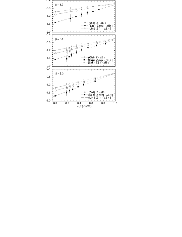
FIG. 2.: The mass dependence of $a_{0}/m_{\pi}(1/{\rm GeV}^{2})$ at each lattice spacing.

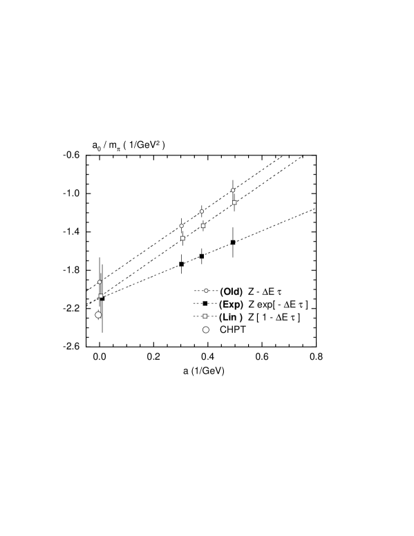
FIG. 3.: $a_{0}/m_{\pi}(1/{\rm GeV}^{2})$ at the chiral limit at each lattice spacing. The CHPT prediction is also plotted.

$\beta=5.9$
$\kappa$	Fit	$\Delta E$	$E^{\prime}$	$a_{0}/m_{\pi}$
$m_{\pi}^{2}\ ({\rm GeV}^{2})$		$(\times 10^{-3})$	$(\times 10^{-5})$	$(1/{\rm GeV}^{2})$
$0.1585$	${\bf Old}$	$12.4(21)$	$-$	$-0.84(12)$
$0.2529(56)$	${\bf Exp}$	$20.9(40)$	$-$	$-1.29(20)$
	${\bf Lin}$	$14.5(19)$	$-$	$-0.96(11)$
	${\bf Sqr}$	$23.1(74)$	$29(21)$	$-1.40(35)$
$0.1580$	${\bf Old}$	$12.5(15)$	$-$	$-0.822(84)$
$0.3468(49)$	${\bf Exp}$	$19.9(27)$	$-$	$-1.20(13)$
	${\bf Lin}$	$14.0(13)$	$-$	$-0.905(72)$
	${\bf Sqr}$	$19.0(57)$	$14(15)$	$-1.16(27)$
$0.1575$	${\bf Old}$	$12.1(12)$	$-$	$-0.786(65)$
$0.4396(48)$	${\bf Exp}$	$18.5(21)$	$-$	$-1.108(98)$
	${\bf Lin}$	$13.3(11)$	$-$	$-0.849(56)$
	${\bf Sqr}$	$16.3(50)$	$8(13)$	$-1.00(24)$
$0.1570$	${\bf Old}$	$11.5(10)$	$-$	$-0.743(55)$
$0.5337(49)$	${\bf Exp}$	$17.0(17)$	$-$	$-1.017(79)$
	${\bf Lin}$	$12.48(92)$	$-$	$-0.794(47)$
	${\bf Sqr}$	$14.4(45)$	$5(12)$	$-0.89(22)$
$0.1565$	${\bf Old}$	$10.86(91)$	$-$	$-0.698(48)$
$0.6297(50)$	${\bf Exp}$	$15.6(15)$	$-$	$-0.931(67)$
	${\bf Lin}$	$11.69(82)$	$-$	$-0.741(42)$
	${\bf Sqr}$	$13.0(41)$	$3(10)$	$-0.81(20)$
$0.1560$	${\bf Old}$	$10.19(82)$	$-$	$-0.654(43)$
$0.7279(51)$	${\bf Exp}$	$14.2(13)$	$-$	$-0.855(59)$
	${\bf Lin}$	$10.92(75)$	$-$	$-0.692(38)$
	${\bf Sqr}$	$11.9(37)$	$2.6(95)$	$-0.74(19)$

TABLE I.: The results at $\beta=5.9$. Four lines for each $m_{\pi}$ are results with the fitting functions ${\bf Old}$, ${\bf Exp}$, ${\bf Lin}$, and ${\bf Sqr}$, which are defined in (5)–(8).

$\beta=6.1$
$\kappa$	Fit	$\Delta E$	$E^{\prime}$	$a_{0}/m_{\pi}$
$m_{\pi}^{2}\ ({\rm GeV}^{2})$		$(\times 10^{-3})$	$(\times 10^{-5})$	$(1/{\rm GeV}^{2})$
$0.15430$	${\bf Old}$	$8.45(98)$	$-$	$-1.13(11)$
$0.1925(42)$	${\bf Exp}$	$13.0(17)$	$-$	$-1.62(17)$
	${\bf Lin}$	$9.82(95)$	$-$	$-1.28(10)$
	${\bf Sqr}$	$14.2(37)$	$9.9(84)$	$-1.73(36)$
$0.15415$	${\bf Old}$	$8.17(79)$	$-$	$-1.080(89)$
$0.2329(42)$	${\bf Exp}$	$12.2(13)$	$-$	$-1.51(13)$
	${\bf Lin}$	$9.38(76)$	$-$	$-1.214(82)$
	${\bf Sqr}$	$13.0(33)$	$8.2(74)$	$-1.59(32)$
$0.15400$	${\bf Old}$	$7.88(71)$	$-$	$-1.035(79)$
$0.2732(42)$	${\bf Exp}$	$11.6(11)$	$-$	$-1.42(11)$
	${\bf Lin}$	$8.97(68)$	$-$	$-1.154(72)$
	${\bf Sqr}$	$12.2(30)$	$7.2(68)$	$-1.48(29)$
$0.15370$	${\bf Old}$	$7.38(62)$	$-$	$-0.960(68)$
$0.3539(44)$	${\bf Exp}$	$10.43(93)$	$-$	$-1.274(89)$
	${\bf Lin}$	$8.23(59)$	$-$	$-1.056(62)$
	${\bf Sqr}$	$11.0(26)$	$6.2(60)$	$-1.33(25)$
$0.15340$	${\bf Old}$	$6.96(56)$	$-$	$-0.987(60)$
$0.4355(46)$	${\bf Exp}$	$9.56(80)$	$-$	$-1.164(76)$
	${\bf Lin}$	$7.73(53)$	$-$	$-0.980(55)$
	${\bf Sqr}$	$10.2(24)$	$5.5(55)$	$-1.22(22)$
$0.15300$	${\bf Old}$	$6.48(49)$	$-$	$-0.831(53)$
$0.5465(49)$	${\bf Exp}$	$8.65(68)$	$-$	$-1.050(65)$
	${\bf Lin}$	$7.12(47)$	$-$	$-0.898(48)$
	${\bf Sqr}$	$9.3(21)$	$4.7(49)$	$-1.11(20)$
$0.15250$	${\bf Old}$	$5.96(43)$	$-$	$-0.760(45)$
$0.6897(52)$	${\bf Exp}$	$7.73(58)$	$-$	$-0.938(56)$
	${\bf Lin}$	$6.48(42)$	$-$	$-0.814(42)$
	${\bf Sqr}$	$8.2(19)$	$3.9(43)$	$-0.99(18)$
$0.15200$	${\bf Old}$	$5.48(40)$	$-$	$-0.697(41)$
$0.8385(55)$	${\bf Exp}$	$6.95(52)$	$-$	$-0.845(50)$
	${\bf Lin}$	$5.92(38)$	$-$	$-0.743(39)$
	${\bf Sqr}$	$7.4(17)$	$3.1(39)$	$-0.89(16)$

TABLE II.: The results at $\beta=6.1$. Four lines for each $m_{\pi}$ are results with the fitting functions ${\bf Old}$, ${\bf Exp}$, ${\bf Lin}$, and ${\bf Sqr}$, which are defined in (5)–(8).

$\beta=6.3$
$\kappa$	Fit	$\Delta E$	$E^{\prime}$	$a_{0}/m_{\pi}$
$m_{\pi}^{2}\ ({\rm GeV}^{2})$		$(\times 10^{-3})$	$(\times 10^{-5})$	$(1/{\rm GeV}^{2})$
$0.15130$	${\bf Old}$	$5.97(60)$	$-$	$-1.21(11)$
$0.1876(36)$	${\bf Exp}$	$8.19(89)$	$-$	$-1.58(14)$
	${\bf Lin}$	$6.71(60)$	$-$	$-1.34(10)$
	${\bf Sqr}$	$7.9(18)$	$2.4(36)$	$-1.54(29)$
$0.15115$	${\bf Old}$	$5.79(48)$	$-$	$-1.160(83)$
$0.2399(36)$	${\bf Exp}$	$7.78(71)$	$-$	$-1.48(11)$
	${\bf Lin}$	$6.43(49)$	$-$	$-1.267(81)$
	${\bf Sqr}$	$7.7(14)$	$2.6(28)$	$-1.48(22)$
$0.15100$	${\bf Old}$	$5.63(42)$	$-$	$-1.115(70)$
$0.2924(36)$	${\bf Exp}$	$7.42(60)$	$-$	$-1.400(93)$
	${\bf Lin}$	$6.19(42)$	$-$	$-1.206(69)$
	${\bf Sqr}$	$7.3(13)$	$2.3(24)$	$-1.39(19)$
$0.15075$	${\bf Old}$	$5.33(36)$	$-$	$-1.042(59)$
$0.3815(38)$	${\bf Exp}$	$6.87(51)$	$-$	$-1.282(76)$
	${\bf Lin}$	$5.80(36)$	$-$	$-1.118(58)$
	${\bf Sqr}$	$6.5(11)$	$1.5(21)$	$-1.23(16)$
$0.15050$	${\bf Old}$	$5.01(33)$	$-$	$-0.973(54)$
$0.4728(40)$	${\bf Exp}$	$6.34(45)$	$-$	$-1.177(67)$
	${\bf Lin}$	$5.42(33)$	$-$	$-1.038(52)$
	${\bf Sqr}$	$5.81(99)$	$0.8(19)$	$-1.10(15)$
$0.15000$	${\bf Old}$	$4.36(30)$	$-$	$-0.842(48)$
$0.6634(45)$	${\bf Exp}$	$5.37(39)$	$-$	$-0.996(58)$
	${\bf Lin}$	$4.70(30)$	$-$	$-0.894(46)$
	${\bf Sqr}$	$4.72(89)$	$0.0(17)$	$-0.90(14)$

TABLE III.: The results at $\beta=6.3$. Four lines for each $m_{\pi}$ are results with the fitting functions ${\bf Old}$, ${\bf Exp}$, ${\bf Lin}$, and ${\bf Sqr}$, which are defined in (5)–(8).

$\beta$	$a\ (1/{\rm GeV})$	${\bf\quad Old}$	${\bf\quad Exp}$	${\bf\quad Lin}$	${\bf\quad Sqr}$
$5.9$	$0.493(7)$	$-0.96(10)$	$-1.51(16)$	$-1.093(90)$	$-1.58(36)$
$6.1$	$0.378(6)$	$-1.185(59)$	$-1.653(80)$	$-1.335(55)$	$-1.78(22)$
$6.3$	$0.302(5)$	$-1.335(76)$	$-1.745(99)$	$-1.466(74)$	$-1.77(21)$
	$a\to 0$	$-1.92(25)$	$-2.09(35)$	$-2.07(24)$	$-2.04(78)$

TABLE IV.: The values of $a_{0}/m_{\pi}(1/{\rm GeV}^{2})$ in the chiral limit for the each fitting function of $R(t)$ at each $\beta$ and those in the continuum limit obtained by liner extrapolation in the lattice spacing. The fitting functions of $R(t)$ are defined in (5)–(8).

REFERENCES

- [1] Y. Kuramashi, M. Fukugita, H. Mino, M. Okawa, and A. Ukawa, Phys. Rev. Lett. 71 (1993) 2387 ; M. Fukugita, Y. Kuramashi, M. Okawa, H. Mino, and A. Ukawa, Phys. Rev. D52 (1995) 3003.
- [2] S.R. Sharpe, R. Gupta, and G.W. Kilcup, Nucl. Phys. B383 (1992) 309.
- [3] R. Gupta, A. Patel, S.R. Sharpe, Phys. Rev. D48 (1993) 388.
- [4] J. Gasser and H. Leutwyler, Phys. Lett. B125 (1983) 325 ; J. Bijnens, G. Colangelo, G. Ecker, J. Gasser, and M.E. Sainio, Phys. Lett. B374 (1996) 210; Nucl. Phys. B508 (1997) 263; G. Colangelo, J. Gasser, and H. Leutwyler, Nucl. Phys. B603 (2001) 125.
- [5] JLQCD Collaboration, S. Aoki et.al., Nucl. Phys. B (Proc. Suppl.) 83 (2000) 241.
- [6] C. Liu, J. Zhang, Y. Chen, and J.P. Ma, Nucl. Phys. B624 (2002) 360.
- [7] JLQCD Collaboration, S. Aoki et.al., Nucl. Phys. B (Proc. Suppl.) 53 (1997) 355.
- [8] M. Lüscher, Commun. Math. Phys. 105 (1986) 153; Commun. Math. Phys. 104 (1986) 177; Selected topics in lattice theory, Lectures given at Les Houches (1988); Nucl. Phys. B354 (1991) 531.
- [9] C. Bernard and M. Golterman, Phys. Rev. D53 (1996) 476.