Blocking of lattice monopoles from the continuum in hot lattice gluodynamics

Abstract:

The abelian monopoles in lattice gluodynamics are associated with continuum monopoles blocked to the lattice. This association allows to predict the lattice monopole action and density of the (squared) monopole charges from a continuum monopole model. The method is applied to the static monopoles in high temperature gluodynamics. We show that the numerical data both for the density and the action of the lattice monopoles can be described in terms of a Coulomb gas of abelian monopoles in the continuum.

1 Introduction

One of the most popular approaches to the problem of confinement of quarks in QCD is the so-called dual superconductor mechanism [1]. The key role in this approach is played by abelian monopoles which are identified with the help of the abelian projection method [2]. The basic idea behind the abelian projections is to fix partially the non-abelian gauge symmetry up to an abelian subgroup. For $\mathop{\rm SU}\nolimits(N)$ gauge theories the residual abelian symmetry group is compact since the original non-abelian group is compact as well. The abelian monopoles arise naturally due to the compactness of the residual gauge subgroup.

In the dual superconductor mechanism the abelian monopoles are considered as effective degrees of freedom which are responsible for confinement of quarks. According to the numerical results [3] the monopoles are condensed in the low temperature (confinement) phase. The condensation of the monopoles leads to formation of the chromoelectric string due to the dual Meissner effect. As a result the fundamental sources of chromoelectric field, quarks, are confined by the string. The importance of the abelian monopoles is also stressed by the existence [4] of the abelian dominance phenomena which was first observed in the lattice $\mathop{\rm SU}\nolimits(2)$ gluodynamics: the monopoles in the so-called Maximal abelian projection [5] make a dominant contribution to the zero temperature string tension (for a review, see ref. [6]).

In the deconfinement phase (high temperatures) the monopoles are not condensed and the quarks are liberated. This does not mean, however, that monopoles do not play a role in non-perturbative physics. It is known that in the deconfinement phase the vacuum is dominated by static monopoles (which run along the “temperature” direction in the euclidean theory) while monopoles running in spatial directions are suppressed. The static monopoles should contribute to the “spatial string tension” — a coefficient in front of the area term of large spatial Wilson loops. And, according to numerical simulations in the deconfinement phase [7], the monopoles make a dominant contribution to the spatial string tension.

In this paper we investigate the physics of the lattice monopole currents in the $\mathop{\rm SU}\nolimits(2)$ gauge theory at high temperatures. The properties of the monopoles are effectively three dimensional due to static nature of the currents. However, the problem which is discussed in this article is quite general and it can not be ascribed only to the three dimensional case which is considered here as a useful and physically relevant example.

The lattice monopoles in Monte Carlo simulations are detected by the standard DeGrand-Toussaint construction [9] which identifies the magnetic monopoles by measuring the magnetic flux coming out of lattice $3D$ cells (cubes). The properties of thus-measured lattice monopoles should obviously depend on the physical size, $b$, of the lattice cell (below we call these lattice objects as “lattice monopoles of the size $b$”). To get the continuum properties of the monopoles one should send the size of the lattice cells to zero, $b\to 0$, what is usually a difficult numerical problem. Here we propose a method — which can be called as “blocking of monopoles from continuum to the lattice” — to identify the couplings of a continuum model for monopoles using the numerical results obtained on the lattice with a finite spacing.

Each lattice $3D$ cell can be considered as a “detector” which measures the magnetic charges of the continuum monopoles travelling through the lattice: if the continuum monopole is located inside a lattice $3D$ cell then the DeGrand-Toussaint method detects a lattice monopole. From this point of view the limit $b\to 0$ is needed to detect accurately the position of the continuum monopole with the help of the lattice detector. If the size of the lattice cell is finite then two or more continuum monopoles may be placed inside the cell. The fluctuations of the monopole charges of the lattice cells should be described by a continuum model. As a result, the lattice observables — such as the vacuum expectation value of the lattice monopole density — should carry information about dynamics of the continuum monopoles. The observables should depend not only on the size of the lattice cell, $b$, but also on features of the continuum model which describes the monopole dynamics. We take the high temperature gluodynamics as a simple example and show that the density and action of the static lattice monopoles of various sizes $b$ can self-consistently be described by a continuum Coulomb gas model.

Our approach resembles the idea of the blocking of the continuum fields to the lattice [10]–[13]. This method allows to construct perfect actions and operators in various field theories. In our paper we are blocking continuum monopoles what is ideologically similar to the blocking of a topological charge [13] and a fermionic current [10, 12] to the lattice. The blocking of the fields, however, leads to a non-integer lattice magnetic current contrary to the quantized lattice definition of the monopole charge [9]. Thus the blocking of topological defects seems to be more suitable for investigation of the lattice monopole charges. There is also a similarity of our approach with the blocking of the lattice monopole degrees of freedom from fine to coarser lattices [14]. This method allows to define a perfect monopole action independent on the spacing of the fine lattice.

To avoid misunderstanding we would like to stress from the very beginning the difference between various lattice monopole sizes $b$. As we mentioned above, we call the size of the lattice $3D$ cell — used for detection of the monopoles — as “the size of the lattice monopole”. This should be distinguished from the physical radius, $r_{0}$, of the monopole core [15] which is obviously independent on the size of the lattice “detector”. In this paper we disregard the existence of the monopole core and consider the continuum monopoles as point-like objects. Thus, we get the finite-sized lattice monopoles by blocking the point-like monopoles from continuum to the lattice.

There is another motivation for our study. Various properties of the lattice monopoles such as the action and density of the monopole currents, depend on the physical size of the lattice monopole [16, 17]. This effect is observed both at zero [16] and finite [17] temperatures. Usually the monopole density is calculated numerically for so called elementary monopoles the size of which coincide with the lattice spacing $a$. Then the monopole quantities in continuum limit ($e.g.$, continuum monopole density) are usually associated with the limit $a\to 0$. However, since the monopole in the gluodynamics has a core of the finite size [15] the continuum monopole may simply “drop” through the lattice cells if $a\ll r_{0}$. Moreover, the scale of the ultraviolet lattice artifacts coincides with the lattice UV cut-off $a$, which, in turn, equal to the size of the elementary monopoles. Therefore the lattice elementary may be affected by the lattice UV artifacts. Both these reasons imply that (at least, naively) there is a possibility that the continuum monopole density may not correctly be calculated as the elementary lattice monopole density in the limit $a\to 0$. One of advantages of our approach is that it allows to relate the lattice monopole quantities to the corresponding physical quantities in continuum limit at the finite lattice spacing making irrelevant the problems noticed above.

The structure of the paper is as follows. In section 2 we derive the lattice monopole action and the density of squared magnetic charges. The basic assumption behind the derivation is that the dynamics of the continuum monopoles — which are blocked to the lattice — is described by the Coulomb gas model. In section 3 we present the numerical results both for the monopole action and for the density of squared magnetic charges. We show that these quantities are in a good agreement with the predictions of section 2. The comparison of the analytical and numerical results allows us to calculate the product of the abelian magnetic screening mass and the monopole density in the continuum model. At the end of section 3 we check the self-consistency of our results as well as validity of the Coulomb gas description for the static monopole currents. Our conclusion is presented in the last section 4.

2 Lattice monopoles from continuum monopoles

In this section we consider the blocking of the continuum monopoles to the lattice in three space-time dimensions. Let us consider a lattice with a finite lattice spacing $b$ which is embedded in the continuum space-time. The cells of the lattice are defined as follows:

$$C_{s}=\left\{b\Bigl{(}s_{i}-\frac{1}{2}\Bigr{)}\leq x_{i}\leq b\Bigl{(}s_{i}+\frac{1}{2}\Bigr{)}\,,\quad i=1,2,3\right\},$$ (1)

where $s_{i}$ is the lattice dimensionless coordinate and $x_{i}$ corresponds to the continuum coordinate.

Each lattice cell, $C_{s}$, detects the total magnetic charge, $k_{s}$, of “continuum” monopoles inside it:

$$k_{s}=\int\limits_{C_{s}}\mbox{d}^{3}x\,\rho(x)\,,\qquad\rho(x)=\sum_{a}q_{a}\,\delta^{(a)}(x-x^{(a)})\,,$$ (2)

where $\rho(x)$ is the density of the continuum monopoles, $x_{a}$ and $q_{a}$ is the position and the charge (in units of a fundamental magnetic charge, $g_{M}$) of $a^{\mathrm{th}}$ continuum monopole. In three dimensions the monopoles are instanton-like objects and the monopole trajectories have zero dimensionality (points). It is worth stressing the difference between continuum and lattice monopoles: the continuum monopoles are fundamental point-like objects in this approach while the lattice monopoles correspond to the lattice cells with non-zero total magnetic charges of continuum monopoles located inside appropriate cells.

According to definitions (2), the lattice monopole charge shares similar properties to the continuum monopole charge. The lattice monopole charge $k_{s}$ is quantized, $k_{s}\in{\mathbb{Z}}$, and conserved in the three-dimensional sense:

$$\sum\limits_{s\in\Lambda}k_{s}\equiv\int\limits_{V}\mbox{d}^{3}x\,\rho(x)=0\,,$$ (3)

if the continuum charge is conserved. Here $\Lambda$ and $V$ denote the lattice and continuum volume occupied by the lattice, respectively. In other words, the total magnetic charge of the lattice monopole configuration is zero on a finite lattice with periodic boundary which is considered in this paper.

Suppose that the dynamics of the continuum monopoles is governed by the $3D$ Coulomb gas model:

$${\cal Z}=\sum\limits_{N=0}^{\infty}\frac{\zeta^{N}}{N!}\Biggl{[}\prod\limits^{N}_{a=1}\int\mbox{d}^{3}x^{(a)}\sum\limits_{q_{a}=\pm 1}\Biggr{]}\exp\left\{-\frac{g^{2}_{M}}{2}\sum_{a,b=1\atop a\neq b}^{N}q_{a}q_{b}\,D\left(x^{(a)}-x^{(b)}\right)\right\}.$$ (4)

The Coulomb interaction in eq. (4) is represented by the inverse laplacian $D$: $-\partial^{2}_{i}D(x)=\delta^{(3)}(x)$. The density of the continuum monopole is assumed to be low. The continuum monopole charges therefore are restricted by the condition $|q_{a}|\leq 1$ which means that these monopoles do not overlap. The average continuum monopole density $\rho$ is controlled by the fugacity parameter $\zeta$.

Note that the model (4) does not exist without properly defined ultraviolet cut-off. Indeed, the self-energy of the point-like monopoles is a linearly divergent function due to the infinite nature of the Coulomb interaction. This divergence — which is not explicitly present in eq. (4) — should appear manifestly in a field representation of the Coulomb gas model which we need below (see, for example, the sin-Gordon representation for the lattice monopole action, eq. (2.1)). The renormalized fugacity is, $\zeta_{\mathrm{ren}}=\zeta\cdot\exp\{g^{2}_{m}/(8\pi\,r_{0})\}$, where the $r_{0}$ is the ultraviolet cut-off. In our case this cut-off is given by the size of the monopole core which is of the order of 0.05 fm at zero temperature [15]. For simplicity we omit the subscript “ren” in the renormalized fugacity below.

The magnetic charges in the Coulomb gas (4) are screened: at large distances the two-point charge correlation function is exponentially suppressed, $\langle\rho(x)\rho(y)\rangle\sim\exp\{-|x-y|/\lambda_{D}\}$. Here $\lambda_{D}$ is the Debye screening length [18],

$$\lambda_{D}=\frac{1}{g_{M}\sqrt{\rho}}\,.$$ (5)

Note that the three dimensional Debye screening length corresponds to a magnetic screening in four dimensions. The density of the continuum monopoles in the leading order is related to fugacity as [18] $\rho=2\zeta$. Below we choose the vacuum expectation value of the continuum monopole density, $\rho$, and the Debye screening length, $\lambda_{D}$, as suitable parameters of the continuum model (instead of $g_{M}$ and $\zeta$).

We are interested in two basic quantities characterizing the lattice monopoles: the lattice monopole action $S_{mon}(k)$ and the v.e.v. of the squared magnetic charge, $\langle k^{2}_{s}\rangle$. We study the quantity $\langle k^{2}_{s}\rangle$ instead of the density, $\langle|k_{s}|\rangle$, since the analytical treatment of the density is difficult while both these quantities are equivalent philosophically.

2.1 Lattice monopole action

To derive the lattice monopole action we substitute the unity,

$$1=\sum_{k(\Lambda)\in{\mathbb{Z}}}\prod_{s\in\Lambda}\delta_{\Lambda}\left(k_{s}-\int\limits_{C_{s}}\mbox{d}^{3}x\,\rho(x)\right),$$ (6)

into eq. (4). Here $\sum_{k(\Lambda)\in{\mathbb{Z}}}\equiv\prod_{s\in\Lambda}\sum_{k_{s}\in{\mathbb{Z}}}$ and $\delta_{\Lambda}$ stands here for the Kronecker symbol ($i.e.$, lattice $\delta$-function). We get

$${\cal Z} = \sum_{k(\Lambda)\in{\mathbb{Z}}}\sum\limits_{N=0}^{\infty}\frac{\zeta^{N}}{N!}\Biggl{[}\prod\limits^{N}_{a=1}\int\mbox{d}^{3}x^{(a)}\sum\limits_{q_{a}=\pm 1}\Biggr{]}\int\limits^{\pi}_{-\pi}{\cal D}_{\Lambda}h\int{\cal D}\chi\times$$ (7)

$$\times\exp\left\{-\int\mbox{d}^{3}x\left[\frac{1}{2g^{2}_{M}}{\bigl{(}\partial_{i}\chi(x)\bigr{)}}^{2}+i\rho(x)\left(\chi(x)-\sum_{s\in\Lambda}\theta_{s}(x)h_{s}\right)+i\sum_{s\in\Lambda}k_{s}h_{s}\right]\right\},\qquad$$

where we have introduced two additional integrations over the continuum field $\chi$ and the compact lattice field $h$ to represent the inverse laplacian in eq. (4) and the Kronecker symbol in eq. (6), respectively. The subscript $\Lambda$ in ${\cal D}_{\Lambda}h$ indicates that the integration is going over the lattice fields $h$. The representative function of the $s^{\mathrm{th}}$ lattice cell is denoted as $\theta_{s}$:

$$\theta_{s}(x)=\left\{\begin{array}[]{ll}1\,,&x\in C_{s}\,,\\ 0\,,&\mbox{otherwise}\,.\\ \end{array}\right.$$ (8)

Summing over the continuum monopole positions according to ref. [18], we get

$$Z=\sum_{k(\Lambda)\in{\mathbb{Z}}}e^{-S_{mon}(k)}\,,$$ (9)

where the lattice monopole action, $S_{\rm mon}$, is defined as follows:

$$e^{-S_{\rm mon}(k)} = \int{\cal D}\chi\int\limits^{\pi}_{-\pi}{\cal D}_{\Lambda}h\exp\Biggl{\{}-\int\mbox{d}^{3}x\Biggl{[}\frac{1}{2g^{2}_{M}}{\bigl{(}\partial_{i}\chi(x)\bigr{)}}^{2}-$$

$$\hphantom{\int{\cal D}\chi\int\limits^{\pi}_{-\pi}{\cal D}_{\Lambda}h\exp\Biggl{\{}-\int\mbox{d}^{3}x\Biggl{[}}-2\zeta\cos\left(\chi(x)-\sum_{s\in\Lambda}\theta_{s}(x)h_{s}\right)+i\sum_{s\in\Lambda}k_{s}h_{s}\Biggr{]}\Biggr{\}}\,.$$

The functional integral over the field $\chi$ in the l.h.s. of this equation resembles the sin-Gordon model coupled to an external source.

Note that the left hand side of eq. (2.1) is invariant both under the global continuum transformations of the field $\chi$, and under the lattice local transformations of the field $h$,

$$\begin{array}[b]{llll}\chi(x)&\to&\chi(x)+2\pi n\,,&\quad n\in{\mathbb{Z}}\\ h_{s}&\to&h_{s}+2\pi m_{s}\,,&\quad m_{s}\in{\mathbb{Z}}\,,\end{array}$$ (13)

respectively. Due to the last invariance we extend below the integration over the lattice field $h$ to infinite limits (this leads to appearance of an inessential factor in front of the partition function).

Let us consider the lattice monopole action in the tree (or, gaussian) approximation. The validity of this approximation is discussed in section 2.2. We expand the cosine function over the small fluctuations in $\chi$ and $h$ and we get in a leading order:

$$e^{-S^{\rm tree}_{\rm mon}(k)} = \int{\cal D}\chi\int\limits^{\pi}_{-\pi}{\cal D}_{\Lambda}h\exp\Biggl{\{}-\int\mbox{d}^{3}x\Biggl{[}\frac{1}{2g^{2}_{M}}{\bigl{(}\partial_{i}\chi(x)\bigr{)}}^{2}+$$

$$\hphantom{\int{\cal D}\chi\int\limits^{\pi}_{-\pi}{\cal D}_{\Lambda}h\exp\Biggl{\{}-\int\mbox{d}^{3}x\Biggl{[}}+\zeta{\left(\chi(x)-\sum_{s\in\Lambda}\theta_{s}(x)h_{s}\right)}^{2}+i\sum_{s\in\Lambda}k_{s}h_{s}\Biggr{]}\Biggr{\}}\,.$$

The integration over field $\chi$ leads to the following expression:

$$e^{-S^{\rm tree}_{\rm mon}(k)}=\int\limits^{\infty}_{-\infty}{\cal D}_{\Lambda}h\exp\Biggl{\{}-\zeta b^{3}\sum_{s,s^{\prime}}h_{s}{\cal F}^{-1}_{s,s^{\prime}}h_{s^{\prime}}+i\sum_{s\in\Lambda}k_{s}h_{s}\Biggr{\}}\,,$$ (15)

where

$${\cal F}^{-1}_{s,s^{\prime}} = \delta_{s,s^{\prime}}-m^{2}_{D}b^{2}{\cal G}_{s,s^{\prime}}\,,$$ (16)

$${\cal G}_{s,s^{\prime}} = \frac{1}{b^{5}}\int\mbox{d}^{3}x\int\mbox{d}^{3}y\theta_{s}(x)\,D_{m_{D}}(x-y)\,\theta_{s^{\prime}}(y)\,,$$ (17)

where $D_{m_{D}}$ is the scalar propagator for a massive particle, $(-\partial^{2}_{i}+m^{2})D_{m}(x)=\delta^{(3)}(x)$, with the Debye mass $m=m_{D}\equiv\lambda^{-1}_{D}$. Note that the lattice operators ${\cal F}$ and ${\cal G}$ are dimensionless quantities.

In eq. (15) the integration over the lattice field $h$ can be performed straightforwardly giving us the action for the lattice monopoles:

$$S^{\rm tree}_{\rm mon}(k)=\frac{1}{4\zeta b^{3}}\sum_{s,s^{\prime}}k_{s}\,{\cal F}_{s,s^{\prime}}k_{s^{\prime}}\,.$$ (18)

Let us calculate the operator ${\cal F}$ on the infinite lattice. We represent the propagator $D_{m_{D}}$ as an integral over continuum momentum and integrating over $x$ and $y$ coordinates in eq. (17):

$${\cal G}_{s,s^{\prime}}=\frac{1}{b^{5}}\int\frac{\mbox{d}^{3}p}{(2\pi)^{3}}\frac{1}{p^{2}+m^{2}_{D}}\,\Biggl{[}\prod^{3}_{i=1}\Biggl{(}\frac{2\sin(bp_{i}/2)}{p_{i}}\Biggr{)}\Biggr{]}e^{i(s-s^{\prime},p)b}\,,$$ (19)

where $(a,b)$ denotes the scalar product of the vector quantities. Changing in eq. (19) the integration variable, $p=q/b$, and introducing the dimensionless mass,

$$\mu=b/\lambda_{D}\,,$$ (20)

we get

$${\cal G}_{s,s^{\prime}}=\int\frac{\mbox{d}^{3}q}{(2\pi)^{3}}\,H(q,\mu)\,e^{i(s-s^{\prime},q)}\,,\qquad H(q,\mu)=\frac{1}{q^{2}+\mu^{2}}\,\prod^{3}_{i=1}{\Biggl{[}\frac{\sin(q_{i}/2)}{q_{i}/2}\Biggr{]}}^{2}\,.$$ (21)

Now we have to find the operator ${\cal F}$ which is inverse to eq. (16). We represent ${\cal F}$ as follows:

$${\cal F}_{s,s^{\prime}}=\int^{\pi}_{-\pi}\mbox{d}^{3}u\,{\cal F}(u)\,e^{i(s-s^{\prime},u)}\,,$$ (22)

Substituting this equation and eq. (16) in the relation,

$$\sum_{s^{\prime\prime}\in\Lambda}{\cal F}^{-1}_{s,s^{\prime\prime}}{\cal F}_{s^{\prime\prime},s^{\prime}}=\delta_{s,s^{\prime}}\,,$$

we get the equation,

$$\int^{\pi}_{-\pi}\mbox{d}^{3}u\,\left\{{\cal F}(u)\left[1-\mu^{2}\sum_{r\in\Lambda}H(u+2\pi r,\mu)\right]-\frac{1}{(2\pi)^{3}}\right\}e^{i(s-s^{\prime},u)}=0\,,$$ (23)

where we have used the Poisson summation formula,

$$\sum_{s^{\prime\prime}\in\Lambda}e^{i(s^{\prime\prime},u-q)}=(2\pi)^{3}\,\sum_{r\in\Lambda}\delta^{(3)}(q-u-2\pi r)\,,$$ (24)

and then integrated over the momentum $q$.

The solution to eq. (23) is

$${\cal F}(u)=\frac{1}{(2\pi)^{3}}\frac{1}{1-\mu^{2}\sum_{r\in\Lambda}H(u+2\pi r,\mu)}\,.$$ (25)

Substituting eq. (25) in eq. (22) and using definition (21), we finally get

$${\cal F}_{s,s^{\prime}}=\int\limits^{\pi}_{-\pi}\frac{\mbox{d}^{3}u}{(2\pi)^{3}}\,{\Biggl{[}\sum_{r(\Lambda)\in{\mathbb{Z}}}\sum_{i=1}^{3}\frac{4\,\sin^{2}(u_{i}/2)}{(\vec{u}+2\pi\vec{r})^{2}+\mu^{2}}\,\prod^{3}_{\stackrel{{\scriptstyle j=1}}{{j\neq i}}}{\Biggl{(}\frac{2\sin(u_{j}/2)}{u_{j}+2\pi r_{j}}\Biggr{)}}^{2}\Biggr{]}}^{-1}\!\!\!\!\!\cdot e^{i(s-s^{\prime},u)}\,,$$ (26)

where we have used the relation

$$\sum_{r_{i}\in{\mathbb{Z}}}\frac{1}{{(u_{i}+2\pi r_{i})}^{2}}=\frac{1}{[4\,\sin^{2}(u_{i}/2)]}\,.$$ (27)

The operator ${\cal F}_{s,s^{\prime}}$ coincides with a three-dimensional perfect propagator for a free scalar field space-time discussed in details in ref. [11].

The summation in eq. (26) over one of the integers $r_{i}$ can explicitly be done with the help of the relation,

$$\sum_{r_{i}\in{\mathbb{Z}}}\frac{1}{(\vec{u}+2\pi\vec{r})^{2}+\mu^{2}}=\frac{1}{2\lambda_{i}(\vec{u}+2\pi\vec{r},\mu)}\frac{\sinh\lambda_{i}(\vec{u}+2\pi\vec{r},\mu)}{\cosh\lambda_{i}(\vec{u}+2\pi\vec{r},\mu)-\cos u_{i}}\,,$$ (28)

where

$$\lambda_{i}(\vec{q},\mu)={\left[\sum^{3}_{\stackrel{{\scriptstyle j=1}}{{j\neq i}}}q^{2}_{j}+\mu^{2}\right]}^{{1}/{2}}\,.$$ (29)

Substituting eq. (28) into eq. (26) we get the final expression for operator ${\cal F}$:

$${\cal F}_{s,s^{\prime}} = \int\limits^{\pi}_{-\pi}\frac{\mbox{d}^{3}u}{(2\pi)^{3}}\,e^{i(s-s^{\prime},u)}\times$$

$$\times\left[\sum_{i=1}^{3}\sum_{r_{j}\in{\mathbb{Z}}\atop j\neq i}\frac{2\,\sin^{2}(u_{i}/2)}{\lambda_{i}(\vec{u}+2\pi\vec{r},\mu)}\frac{\sinh\lambda_{i}(\vec{u}+2\pi\vec{r},\mu)}{\cosh\lambda_{i}(\vec{u}+2\pi\vec{r},\mu)-\cos u_{i}}\cdot\prod^{3}_{k=1\atop k\neq i}\frac{4\sin^{2}(u_{k}/2)}{(u_{k}+2\pi r_{k})^{2}}\right]^{-1}\,.$$

The leading term in the lattice monopole action is defined by eqs.(18), (2.1).

The finite-volume expression for the lattice monopole action can be obtained from eq. (2.1) by the standard substitution:

$$u_{i}\to\frac{2\pi k_{i}}{L_{i}}\,,\qquad k=0\,,1\,,\dots L_{i}-1\,,\qquad\int\limits^{\pi}_{-\pi}\frac{\mbox{d}u_{i}}{2\pi}\to\frac{1}{L_{i}}\sum\limits_{k_{i}=0}^{L_{i}-1}\,,$$ (31)

where $L_{i}$ is the lattice size in $i^{\mathrm{th}}$ direction.

In the infinite-volume case the lattice operator ${\cal F}_{s,s^{\prime}}$ depends only on the dimensionless quantity $\mu$, eq. (20), which is the ratio of the lattice monopole size $b$ and the Debye screening length, eq. (5). As we will see below the form of the operator ${\cal F}$ is qualitatively different in the limits of small and large $\mu$. Thus the Debye length $\lambda_{D}$ sets a scale for the lattice monopole size (or, better to say, for the size of the lattice cell) which characterizes different forms of the lattice monopole action.

2.1.1 Action for large lattice monopoles

Let us consider the case of the large lattice monopoles, $b\gg\lambda_{D}$, or, equivalently, $\mu\gg 1$. In this case eq. (2.1) can be simplified since functions $\lambda_{i}$ (eq. (29)) are large and $\sinh\lambda_{i}\sim\cosh\lambda_{i}\sim e^{\lambda_{i}}/2$. Up to $O(e^{-\mu})$ corrections the operator ${\cal F}_{s,s^{\prime}}$ is given by

$${\cal F}_{s,s^{\prime}}(\mu\gg 1)=\int\limits^{\pi}_{-\pi}\frac{\mbox{d}^{3}u}{(2\pi)^{3}}\,{\left[\sum_{i=1}^{3}\sum_{r_{j}\in{\mathbb{Z}}\atop j\neq i}\frac{2\sin^{2}(u_{i}/2)}{\lambda_{i}(u,\mu)}\prod^{3}_{k=1\atop k\neq i}\frac{4\sin^{2}(u_{k}/2)}{(u_{k}+2\pi r_{k})^{2}}\right]}^{-1}\!\!\!\!\cdot e^{i(s-s^{\prime},u)}\,.$$ (32)

In the case of large $\mu$, the function $\lambda_{i}$ in eq. (29) is close to $\mu$ for all $r_{i}\ll\mu/(2\pi)$. The deviation of $\lambda$ from $\mu$ becomes substantial only for terms with large summation variable $r_{i}$, $r_{i}\gg\mu/(2\pi)$. However such large $r_{i}$’s are in any case suppressed as $\sim\prod_{j\neq i}{(2\pi r_{j})}^{-2}$ according to eq. (32). Therefore the approximation $\lambda_{i}=\mu$ would lead only to $O(\mu^{-2})$ corrections in eq. (32). Up to these corrections eq. (32) reads as follows:

$${\cal F}_{s,s^{\prime}}(\mu\gg 1)=\frac{\mu}{2}\int\limits^{\pi}_{-\pi}\frac{\mbox{d}^{3}u}{(2\pi)^{3}}\,{\left[\sum_{i=1}^{3}\sin^{2}\left(\frac{u_{i}}{2}\right)\prod^{3}_{j=1\atop j\neq i}\sum_{r_{j}\in{\mathbb{Z}}}\frac{4\sin^{2}(u_{j}/2)}{(u_{j}+2\pi r_{j})^{2}}\right]}^{-1}\!\!\!\!\cdot e^{i(s-s^{\prime},u)}\,.$$ (33)

In turn, eq. (33) can be simplified with the help of the relation (27), giving:

$${\cal F}_{s,s^{\prime}}(\mu\gg 1)=2\mu\,D_{s,s^{\prime}}\,,$$ (34)

where $D_{s,s^{\prime}}$ is the lattice laplacian:

$$D_{s,s^{\prime}}=\int\limits^{\pi}_{-\pi}\frac{\mbox{d}^{3}u}{(2\pi)^{3}}\,{\left[4\sum\limits_{i=1}^{3}\sin^{2}\left(\frac{u_{i}}{2}\right)\right]}^{-1}\,e^{i(s-s^{\prime},u)}\,.$$ (35)

Thus for large sizes of the lattice cells, $b\gg\lambda_{D}$, the lattice monopole action (18) is of the Coulomb-type:

$$S^{\rm tree}_{\rm mon}(k)=C(b)\,\sum\limits_{s,s^{\prime}}k_{s}\,D_{s,s^{\prime}}\,k_{s^{\prime}}+O\left(\left(\frac{\lambda_{D}}{b}\right)^{4}\right)\,,\quad b\gg\lambda_{D}\,.$$ (36)

The pre-Coulomb term $C$ can be expressed through the continuum density of the monopoles, $\rho$, the Debye screening length $\lambda_{D}$ and the lattice spacing $b$ as

$$C(b)=\frac{1}{\lambda_{D}\rho}\cdot\frac{1}{b^{2}}\,.$$ (37)

Here we used eq. (20).

Thus in the limit of large lattice monopole sizes, $b$, the lattice monopole action is of the Coulomb form. The long-range nature of the Coulomb interaction in the effective lattice action and the screening effect in the underlying high temperature theory do not contradict each other as one may think. The analog of this situation in continuum can be represented by a similar Coulomb gas model (4) which contain the long-range interaction part in the lagrangian. However, the interactions between monopoles lead to the screening effect in various correlators in this model. Obviously, the lattice Coulomb gas model (36) must also possess the screening effect despite the long range nature of the Coulomb term in the action.

The coefficient in front of the Coulomb term, $C(b)$, scales as $C(b)\sim b^{-2}$. Note that this form of scaling is a non-perturbative effect. Indeed, naively one could expect that this coefficient has to be proportional to the (squared) renormalized magnetic charge in three dimensions, $C(b)\sim g^{2}_{M}$. The magnetic charge is inversely proportional to the $3D$ electric charge, $g_{M}\sim g^{-1}_{E,3D}$. In the leading (tree) order of dimensional reduction formalism the electric charge is given by $g_{E,3D}=g_{4D}(\Lambda,T)\cdot\sqrt{T}$, where $T$ is the temperature, $g_{4D}$ is the running $4D$ charge of the $\mathop{\rm SU}\nolimits(2)$ gluodynamics and $\Lambda$ is the renormalization scale. As a result, $C(b)\sim{[\,g^{2}_{4D}(\Lambda,T)\,T\,]}^{-1}$. The size of the lattice monopole, $b$, may enter the above expression only in the form of the renormalization scale, $\Lambda\sim 1/b$. However, this would lead only to logarithmic $b$-dependence of the coefficient $C(b)$. Thus the $b^{-2}$ dependence of the pre-Coulomb coefficient is clearly of a non-perturbative nature.

2.1.2 Action for small lattice monopoles

In the case of small lattice monopoles the leading term of the operator ${\cal F}$ for $b\ll\lambda_{D}$ follows immediately from eq. (16): $F_{s,s^{\prime}}=\delta_{s,s^{\prime}}$. Thus the monopole action (18) becomes:

$$S^{\rm tree}_{\rm mon}(k)=M(b)\,\sum\limits_{s}k^{2}_{s}+O\left(\left(\frac{b}{\lambda_{D}}\right)^{2}\right)\,,\qquad b\ll\lambda_{D}\,,$$ (38)

where the coefficient

$$M(b)=\frac{1}{4{\rho}}\cdot\frac{1}{b^{3}}\,,$$ (39)

plays a role of the lattice monopole mass. Indeed, the leading term in the action for $N$ small lattice monopoles with the charges $q=\pm 1$ is $S=M(b)\cdot N$.

In summary, we have established that the monopole action depends on the ratio of the lattice cell and the continuum Debye screening mass, $b/\lambda_{D}$:

$$S_{\rm mon}(k)=\left\{\begin{array}[]{lll}\displaystyle\frac{1}{4\rho}\cdot\frac{1}{b^{3}}\cdot\sum\limits_{s}k^{2}_{s}+\cdots\,,&\qquad b\ll\lambda_{D}\,;\\ \displaystyle\frac{1}{\rho\,\lambda_{D}}\cdot\frac{1}{b^{2}}\cdot\sum\limits_{s,s^{\prime}}k_{s}\,D_{s,s^{\prime}}\,k_{s^{\prime}}+\cdots\,,&\qquad b\gg\lambda_{D}\,,\end{array}\right.$$ (42)

where $D_{s,s^{\prime}}$ is the inverse laplacian on the lattice. Thus the leading contribution to the lattice monopole action is given by the mass (Coulomb) terms for small (large) lattice monopoles.

2.2 Validity of the gaussian approximation

As we will see below, from the point of view of numerical computations the most interesting and reliable case corresponds to the large-$b$ monopoles. Here we briefly discuss the validity of the gaussian approximation in this limit. The detailed derivation will be given elsewhere [19].

We have truncated the cosine function in eq. (2.1) and performed the gaussian integration over the continuum field $\chi$ in eq. (2.1) to get the effective action in the leading order for the lattice field $h_{s}$. This action appears under the exponential function in eq. (15). The integration over the lattice fields $h$ led us to the Coulomb action (36) for the lattice monopoles in the large-$b$ limit. Let estimate the Coulomb action (36) coming from the next order of the truncation of the cosine function in eq. (2.1).

Expanding the cosine function in eq. (2.1) up to the fourth order and treating the correction as a perturbation we arrive to the following correction to the monopole action,

$$\delta S^{(4)}_{\rm mon}(k)=-\frac{\zeta}{12}\,\int\mbox{d}^{3}x\,\left\langle{\left(\chi(x)-\sum_{s\in\Lambda}\theta_{s}(x)h_{s}\right)}^{4}\right\rangle,$$ (43)

where we used the superscript “$(4)$” because, as we show below, this action contains, $O(k^{4})$ monopole-monopole interactions. The quantum average (43) is taken in the partition function (2.1) containing the monopole current $k$ as a source.

Integrating the fields $\chi$ and $h$, and neglecting independent of $k$ terms we arrive to the following $k^{4}$-correction to the monopole action:

$$\delta S^{(4)}_{\rm mon}(k) = -\frac{1}{192\,\zeta^{3}\,b^{9}}\sum\limits_{s_{1},\dots,s_{4}}k_{s_{1}}\dots k_{s_{4}}\,D_{s_{1},\dots,s_{4}}\,,$$

$$D_{s_{1},\dots,s_{4}} = \sum\limits_{s^{\prime}_{1},\dots,s^{\prime}_{4}}{\cal F}_{s_{1},s^{\prime}_{1}}\dots{\cal F}_{s_{4},s^{\prime}_{4}}\,Y_{s^{\prime}_{1},\dots,s^{\prime}_{4}}\,,$$ (44)

where

$$Y_{s^{\prime}_{1},\dots,s^{\prime}_{4}} = {\left[\prod\limits^{4}_{a=1}\int\frac{\mbox{d}^{3}q^{(a)}}{{(2\pi)}^{3}}\frac{q^{(a),2}}{q^{(a),2}+\mu^{2}}\right]}\,{(2\pi)}^{3}\,\delta^{(3)}\Bigl{(}q^{(1)}+\cdots+q^{(4)}\Bigr{)}\times$$ (45)

$$\times{\left[\prod^{3}_{i=1}\frac{\sin(q^{(a)}_{i}/2)}{q^{(a)}_{i}/2}\right]}\cdot\exp\left\{i\sum^{4}_{b=1}q^{(b)}s_{b}\right\}.$$

The operator $Y$ is a converging function both in the limits of large and small $q$.

According to eq. (34) the operator ${\cal F}$ is proportional to the first power of $b$ in the limit $\mu\equiv m_{D}b\gg 1$. The estimation of the operator $Y$, eq. (45), is difficult even in the limit of large $b$. However, one can notice that $Y$ contains the dependence on $b$ in the denominators under the integrals over $q$, and, similarly to the operator ${\cal F}^{-1}$, the operator $Y$ should not be a rising function of the scale $b$. Estimating $Y$ as being of the order of unity, we get: $|S^{(4)}_{\rm mon}(k)|\lesssim g^{4}_{M}/(48\zeta b^{5})O(k^{4})$. Thus, in the limit $b\to\infty$ the action $S^{(4)}_{\rm mon}$ provides a small correction to the Coulomb action (36), which is proportional to $b^{-2}$. These results are confirmed by the fact that in the limit of large monopoles $k^{4}$ correction to the monopole action is small compared to the quadratic terms, ref. [17]. Moreover, as we will see below, our numerical calculations shows that the quadratic part of the monopole action can be described by the Coulomb interactions with a high accuracy.

2.3 Lattice monopole density

In this section we discuss the dependence of the density of the extended lattice monopoles on the monopole size $b$. The simplest quantity characterizing the monopoles is the monopole density $\rho_{latt}(b)$ measured in the lattice units:

$$\rho_{\rm latt}(b)=\frac{1}{L^{3}}\,\left\langle\sum_{s\in\Lambda}|k_{s}|\right\rangle,$$ (46)

where $L$ is the lattice size in units of $b$. However, the treatment of eq. (46) from the analytical point of view is more difficult than that of the squared density of the squared lattice monopole charges:

$$\langle k^{2}(b)\rangle=\frac{1}{L^{3}}\,\left\langle\sum_{s\in\Lambda}k^{2}(s)\right\rangle.$$ (47)

Below we discuss the quantity (47) which has a similar physical meaning to the lattice monopole density (46).

Both in eq. (46) and eq. (47) the value of $k_{s}$ is equal to the total magnetic charge of the continuum monopoles which are placed inside the corresponding cube of the volume $b^{3}$. Obviously the lattice density (46) does not give the correct density of the continuum monopoles in general since if the lattice monopole size is large enough then the oppositely charged continuum monopoles cancel fields of each other inside the cell $C_{s}$. Moreover, the dependence of the densities (46) and (47) on the lattice monopole size $b$ must reflect the dynamics of the continuum monopoles. Indeed, one can expect that the functions $\rho_{\rm latt}(b)$ for the Coulomb monopole gas and for the random monopole ensembles should differ from each other since the inter-monopole correlations are absent in the latter case contrary to the former one. As we will see below the situation is similar to the lattice monopole action discussed in the previous section.

Using eq. (2) the lattice density (47) can be written in the continuum theory as follows:

$$\langle k^{2}\rangle=\int_{C_{s}}\mbox{d}^{3}x\int_{C_{s}}\mbox{d}^{3}y\,\langle\rho(x)\,\rho(y)\rangle\,,$$ (48)

where the lattice site $s$ is fixed and the average is taken in the Coulomb gas of the magnetic monopoles described by the partition function (4). We assume the validity of the dilute gas approximation for the continuum monopoles.

The correlator of the continuum monopole densities, $\langle\rho(x)\,\rho(y)\rangle$, is well known from ref. [18]. Introducing the source for the magnetic monopole density, $J$, eq. (48) can be rewritten as follows:

$$\langle k^{2}\rangle=-\int_{C_{s}}\mbox{d}^{3}x\int_{C_{s}}\mbox{d}^{3}y\,\frac{\delta^{2}}{\delta J(x)\,\delta J(y)}\left\langle\exp\left\{i\int\mbox{d}^{3}z\rho(z)\,J(z)\right\}\right\rangle{\biggl{|}}_{J=0}\,.$$ (49)

Then we repeat the transformations in the previous section which led us to eq. (2.1). Integrating over quadratic fluctuations of the field $\chi$ we get in the leading order

$$\langle\rho(x)\,\rho(y)\rangle=\rho\,\left[\delta^{(3)}(x-y)-m^{2}_{D}D_{m_{D}}(x-y)\right].$$ (50)

Substituting eq. (50) in eq. (48) and taking the integrals over the cell $C_{s}$ we get

$$\langle k^{2}\rangle=\rho\,b^{3}\,P(\mu)\,,$$ (51)

where $\mu$ is the dimensionless Debye mass, eq. (20) and in the thermodynamical limit the function $P$ is

$$P(\mu)\equiv{({\cal F}^{-1})}_{0,0}(\mu)=1-\mu^{2}\,\int\frac{\mbox{d}^{3}\,q}{{(2\pi)}^{3}}\,H(q,\mu)\,.$$ (52)

Here the inverse matrix ${\cal F}_{s,s^{\prime}}$ is given by eq. (16) and the function $H$ is defined in eq. (21). The finite-volume analog of eq. (52) can be easily written using the substitution (31). Note that eq. (51), (52) establish a direct relation between the density of the squared lattice monopole charges and the lattice monopole action, eq. (18).

It is interesting to study the scaling laws of the lattice monopole densities for large and small monopoles. In the limiting cases the behaviour of the function $P$ is as follows:

$$P(\mu)=\left\{\begin{array}[]{ll}C_{1}\,\mu^{-1}+O(\mu^{-3})\,,&\qquad\mu\to\infty\,,\\ 1-C_{2}\mu^{2}+O(\mu^{4})\,,&\qquad\mu\to 0\,,\end{array}\right.$$ (55)

where the constants $C_{1,2}$ are

$$C_{1}\approx 2.94\,,\qquad C_{2}=\int\frac{\mbox{d}^{3}q}{{(2\pi)}^{3}}\,H(q,0)\approx 0.148\,.$$ (56)

Substituting the asymptotic functions (55) in eq. (51) we get the scaling laws (in physical units) for the density of the squared lattice monopole charge:

$$\langle k^{2}\rangle=\left\{\begin{array}[]{ll}C_{1}\,\rho\,\lambda_{D}\,b^{2}\cdot\left[1+O\left({\left(\lambda_{D}/b\right)}^{2}\right)\right]\,,&\qquad b\gg\lambda_{D}\,,\\ \rho\,b^{3}\cdot\left[1+C_{2}\,\rho\,{(b/\lambda_{D})}^{2}\,+O\left({\left(b/\lambda_{D}\right)}^{4}\right)\right]\,,&\qquad b\ll\lambda_{D}\,.\end{array}\right.$$ (59)

One can note some interesting properties of the density of the squared magnetic charge, eq. (59).

1. The dependence of the lattice monopole charge squared on the monopole size $b$ is always polynomial, $b^{n}$. In particular, this property is remarkable in the large-$b$ region: one may expect that the screening of the monopole charges in the magnetic monopole plasma would lead to an exponential behaviour, $e^{-\mbox{const.}\,m_{D}\,b}$, which is not the case.

2. As in the case of the lattice monopole action, the power $n$ of the leading scaling law depends crucially on the value of the ratio of the lattice monopole size and the Debye screening length.

3. The proportionality of the density $\langle k^{2}\rangle$ to $b^{2}$ in large-$b$ region has a simple explanation. In a random gas of continuum monopoles we would get $\langle k^{2}\rangle\sim\rho\,b^{3}$ since the monopoles are not correlated with each other. In the Coulomb gas the monopoles are correlated and moreover, screened. Therefore the monopoles separated from the boundary of the cell by the distance larger than $\lambda_{D}$, do not contribute to $\langle k^{2}\rangle$. Consequently, the $b^{3}$ proportionality for the random gas turns into $\lambda_{D}b^{2}$ in the Coulomb gas and we get $\langle k^{2}\rangle\sim\rho\,\lambda_{D}\,b^{2}$. The coefficient of proportionality is of a geometrical origin.

4. In the small $b$ region the density of the squared lattice monopole charges is equal to the density of the continuum monopoles times the volume of the cell. This is natural, since the smaller volume of the lattice cell, $b^{3}$, the smaller chance for two continuum monopoles to be located at the same cell. Therefore each cell predominantly contains not more that one continuum monopole, which leads to the relation $k^{2}_{s}=|k_{s}|=0,1$. As a result we get $\langle k^{2}\rangle\to\rho_{\rm latt}(b)\to\rho\,b^{3}$ in the limit $b\to 0$.

Closing this section we mention interesting relations between the density of the small- and large- sized lattice monopoles and the coefficients in front of, respectively, the mass and the Coulomb terms of the monopole action, eqs.(42), (59):

$$C(b)=\frac{C_{1}}{\langle k^{2}(b)\rangle}\,,\qquad b\gg\lambda_{D}\,,\qquad\hbox{and}\qquad M(b)=\frac{1}{4\,\langle k^{2}(b)\rangle}\,,\qquad b\ll\lambda_{D}\,.$$ (60)

All these results are obtained in the gaussian approximation. The results on next to the leading order correction to the action and the monopole density will be published elsewhere [19].

3 Numerical results

3.1 Details of simulations

In order to get perfect lattice monopole action and density we perform numerically blockspin transformations for the lattice monopole currents. The original model is define on the fine lattice with the lattice spacing $a$ and after the blockspin transformation, the renormalized lattice spacing becomes $b=na$, where $n$ is the number of steps of blockspin transformations. The continuum limit is taken as the limit $a\to 0$ and $n\to\infty$ for a fixed physical scale $b$.

Finite temperature system possesses a periodic boundary condition for time direction and the physical length in the time direction is limited to less than $1/T$. In this case it is useful to introduce anisotropic lattices. In the space direction, we perform the blockspin transformation and the continuum limit is taken as $a_{s}\to 0$ and $n_{s}\to\infty$ for a fixed physical scale $b=n_{s}a_{s}$. Here $a_{s}$ is the lattice spacing in the space directions and $n_{s}$ is the blockspin factor. In the time direction, the continuum limit is taken as $a_{t}\to 0$ and $N_{t}\to\infty$ for a fixed temperature $T=1/(N_{t}a_{t})$. Here $a_{t}$ is the lattice spacing in the time direction and $N_{t}$ is the number of lattice sites for the time direction. After taking the continuum limit, we finally get the effective lattice monopole action which depends on the physical scale $b$ and the temperature $T$.

In this paper the numerical procedure to generate the field configurations is identical to the one used ref. [17]. While referring an interested reader to the above paper, here we mention for completeness briefly the basic points of our numerical procedure. The anisotropic Wilson action for pure four-dimensional $\mathop{\rm SU}\nolimits(2)$ QCD is written as

$$S = \beta\left\{\frac{1}{\gamma}\sum_{s,i>j\neq 4}P_{ij}(s)+\gamma\sum_{s,i\neq 4}P_{i4}(s)\right\},$$

$$P_{\mu\nu}(s) \equiv \frac{1}{4}\mathop{\rm Tr}\nolimits\left[\mathbbm{1}-U_{\mu}(s)U_{\nu}(s+\hat{\mu})U_{\mu}^{\dagger}(s+\hat{\nu})U_{\nu}^{\dagger}(s)\right]+\hbox{h.c.}$$ (61)

If $\gamma=1$, the lattice is isotropic $(a_{s}=a_{t})$. We can consider various lattice spacings $a_{s}$ and $a_{t}$ by varying the parameters $\beta$ and $\gamma$ in the action. The procedure to determine the relation between the lattice spacings $a_{s}$, $a_{t}$ and the parameters $\beta$, $\gamma$ is described in details in ref. [17]. Using the parameters which are determined in ref. [17], we simulate the pure four-dimensional $\mathop{\rm SU}\nolimits(2)$ QCD on the lattice $48^{3}\times L_{t}$ with $L_{t}=12,10,8,6,4$ corresponding to temperature $T/T_{c}=1.6,1.92,2.4,3.2,4.8$. The parameters used here are summarized in Table 1. The scaling behaviors for time-like lattice monopole action at above mentioned lattices show in large $b$ region [17].

$\beta$	$\gamma$	$a_{s}$	$a_{t}$	$\beta$	$\gamma$	$a_{s}$	$a_{t}$
2.470	2.841	0.250	0.075	2.565	2.152	0.180	0.075
2.500	2.615	0.225	0.075	2.573	2.098	0.175	0.075
2.533	2.354	0.200	0.075	2.581	2.042	0.170	0.075
2.548	2.256	0.190	0.075	2.598	1.927	0.160	0.075

Table 1: Parameters $\beta,\gamma$ and corresponding lattice spacings $a_{s},a_{t}$ in units of the zero-temperature string tension, $\sqrt{\sigma_{T=0}}$.

To study the abelian monopole dynamics we generate the thermalized non-abelian link fields $\{U_{\mu}(s)\}$ and we perform abelian projection in the Maximally abelian (MA) gauge [5] for each $\mathop{\rm SU}\nolimits(2)$ configuration. The MA gauge fixing condition is the maximization of the quantity $R$,

$$\max\limits_{\Omega}R[U^{(\Omega)}]\,,\qquad R[U]={\mathop{\rm Tr}\nolimits}\sum_{s,\mu}\left[U_{\mu}(s)\sigma_{3}U_{\mu}^{\dagger}(s+\hat{\mu})\sigma_{3}\right].$$ (62)

under the $\mathop{\rm SU}\nolimits(2)$ gauge transformations, $U\to U^{(\Omega)}=\Omega^{\dagger}U\Omega$. The gauge fixing condition (62) is invariant under an abelian subgroup of the group of the $\mathop{\rm SU}\nolimits(2)$ gauge transformations. Thus the condition (62) corresponds to the partial gauge fixing, $\mathop{\rm SU}\nolimits(2)\to\mathop{\rm{}U}\nolimits(1)$.

After the MA gauge fixing, the abelian, $\{u_{\mu}(s)\}$, and non-abelian $\{\tilde{U}_{\mu}(s)\}$ link fields are separated, $\tilde{U}_{\mu}(s)=C_{\mu}(s)u_{\mu}(s)$ , where

$$C_{\mu}(s)=\pmatrix{\sqrt{1-|c_{\mu}(s)|^{2}}&-c_{\mu}^{\ast}(s)\cr c_{\mu}(s)&\sqrt{1-|c_{\mu}(s)|^{2}}},\qquad u_{\mu}(s)=\pmatrix{e^{i\theta_{\mu}(s)}&0\cr 0&e^{-i\theta_{\mu}(s)}}.$$ (63)

The vector fields $C_{\mu}(s)$ and $u_{\mu}(s)$ transform like a charged matter and, respectively, a gauge field under the residual $\mathop{\rm{}U}\nolimits(1)$ symmetry. Next we define a lattice monopole current (DeGrand-Toussaint monopole) [9]. Abelian plaquette variables $\theta_{\mu\nu}(s)$ are written as

$$\theta_{\mu\nu}(s)=\theta_{\mu}(s)+\theta_{\nu}(s+\hat{\mu})-\theta_{\mu}(s+\hat{\nu})-\theta_{\nu}(s)\,,\qquad(-4\pi<\theta_{\mu\nu}(s)\leq 4\pi)\,.$$ (64)

It is decomposed into two terms using integer variables $n_{\mu\nu}(s)$:

$$\theta_{\mu\nu}(s)\equiv\bar{\theta}_{\mu\nu}(s)+2\pi n_{\mu\nu}(s)\,,\qquad(-\pi<\bar{\theta}_{\mu\nu}(s)\leq\pi).$$ (65)

Here $\bar{\theta}_{\mu\nu}(s)$ is interpreted as an electromagnetic flux through the plaquette and $n_{\mu\nu}(s)$ corresponds to the number of Dirac string piercing the plaquette. The lattice monopole current is defined as

$$k_{\mu}(s)=\frac{1}{2}\epsilon_{\mu\nu\rho\sigma}\partial_{\nu}n_{\rho\sigma}(s+\hat{\mu})\,.$$ (66)

It satisfies the conservation law $\partial_{\mu}^{\prime}k_{\mu}(s)=0$.

To study numerically the lattice monopoles of various lattice sizes we use the so-called extended monopole construction [20]. At zero temperature the extended monopoles can be defined in the symmetric way. They have the physical size $b^{3}$ where $b=na$. The charge of the $n$-blocked monopole is equal to the sum of the charges of the elementary lattice monopoles inside the $n^{3}$ lattice cell. At finite temperature the blocking of spatial and temporal currents should be done separately [17]:

$$K_{\mu\neq 4}(s_{s},s_{4}) = \sum_{i,j=0}^{n_{s}-1}\sum_{l=0}^{n_{t}-1}k_{\mu\neq 4}\left(n_{s}s_{s}+(n_{s}-1)\hat{\mu}+i\hat{\nu}+j\hat{\rho},n_{t}s_{4}+l\right),$$

$$K_{4}(s_{s},s_{4}) = \sum_{i,j,l=0}^{n_{s}-1}k_{4}\left(n_{s}s_{s}+i\hat{\mu}+j\hat{\nu}+l\hat{\rho},n_{t}s_{4}+(n_{t}-1)\right),$$ (67)

where $n_{s}$ ($n_{t}$) is the number of blocking steps in space (time) direction.

We consider only the $n_{t}=1$ case since we are interested in high temperatures for which the monopoles are almost static. The lattice blocking is performed only in spatial directions, $n_{s}=1\dots 8$, and we study only the static components $K_{4}$ among the $4D$ monopole currents $K_{\mu}$ (below we denote $K_{4}$ as $k$.). At high temperature we disregard the spatial currents $K_{i}$ since they are not interesting from the point of view of the long-range non-perturbative spatial physics. The size of the lattice monopoles is measured (unless otherwise specified) in terms of the zero temperature string tension, $\sigma_{T=0}$.

In order to figure out whether the continuum monopole currents can be described by the Coulomb gas model we should compare Monte Carlo results with the appropriate analytical predictions derived in the previous section. In principle this should allow us to obtain all independent parameters of the Coulomb gas (the continuum monopole density and the Debye screening length). However, the lattice monopoles of small sizes are largely affected by the lattice artifacts since in this case the number of blocking steps is small and possible magnetic charges of such monopoles are restricted due to peculiarities of the DeGrand-Toussaint definition [9]. Moreover, the short-range interaction between the continuum monopoles should deviate from the simple Coulomb law due to a non-zero finite radius of the abelian monopole [15]. Thus in order to get reliable results we perform the comparison of the numerical data with analytical predictions for sufficiently large blocking steps only. The restriction to large-$b$ region allows us to calculate the product of the continuum monopole density and the Debye screening length,

$$R(T)=\lambda_{D}(T)\,\rho(T)\,,$$ (68)

while a separate calculation of these quantities is not possible. Nevertheless the knowledge of quantity is enough to make a conclusion about realization of the Coulomb gas picture for static continuum monopole lines. In subsections 3.2 and 3.3 we get the quantity $R$ from the lattice monopole action and density, respectively. To avoid confusion we denote $R$ in these cases as $R_{act}$ and $R_{\rho}$, correspondingly. In subsection 3.4 we check the consistency of the obtained values of $R_{act}$ and $R_{\rho}$ with each other and with the Coulomb gas picture.

3.2 Lattice monopole action

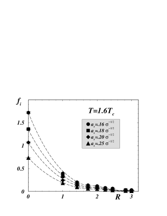
Figure 1: The coupling constants, $f_{i}$, of the lattice monopole action $vs.$ the distance, $r$ at $T=1.6T_{c}$ for various spacings of the fine lattice, $a_{s}$. The fits (70) are visualized by the dashed lines.

The lattice monopole action for the static monopole currents, $k_{s}$, at high temperatures was found numerically in ref. [17] using an inverse Monte-Carlo procedure. It turns out that the self-interaction of the temporal lattice currents can be successfully described by the quadratic monopole action:

$$S_{\rm mon}(k)=\sum_{i}f_{i}\,S_{i}(k)\,,$$ (69)

where $S_{i}$ are two-point operators of the lattice monopole charges corresponding to different separations between the charges. The term $S_{1}$ corresponds to the zero distance between the lattice monopoles, $S_{2}$ corresponds to the unit distance and so on (see ref. [17] for further details).

The two-point coupling constants, $f_{i}$, of the lattice monopole action are shown in figures 1 and 2 as a function the distance between the lattice points. The numerical data corresponds to lowest, $T=1.6T_{c}$, and highest, $T=4.8T_{c}$, available temperatures. The number of blocking steps is fixed to $n_{s}=6$ while the spatial spacings of the fine lattice, $a_{s}$, are available for a set of values ranging from $a_{s}=.16\sigma^{-1/2}$ till $a_{s}=.25\sigma^{-1/2}$.

Figure 2: The same as in figure 1 but for the temperature $T=4.8T_{c}$.

According to eq. (42) the leading term in the lattice monopole action for large lattice monopoles ($b\gg\lambda_{D}$) must be proportional to the Coulomb interaction,

$$S_{\rm mon}(k)=C_{C}\cdot\sum\limits_{s,s^{\prime}}k_{s}\,D_{s,s^{\prime}}\,k_{s^{\prime}}\,.$$ (70)

To check this prediction we fit the coupling constants $f_{i}$ by the Coulomb interaction (70) treating $C_{C}$ is the fitting parameter. The fits are visualized by the dashed lines in figures 1 and 2.

As one can see from the figures, this one-parametric fit works very good. The $\chi^{2}/d.o.f.$ parameter is of the order of unity for most fits while it is of order of 2 for the smallest lattice spacing, $a\sqrt{\sigma}=0.16$. Note that the dependence of the lattice Coulomb interaction on the distance between the interaction points is not a monotonic function, as one can see from the fitting curves. Similar non-monotonic behaviour is also observed in the numerical data.

Using the fitting of the action we obtain the values of $C_{C}$ for various sizes of the lattice monopole, $b\sqrt{\sigma}=.96\dots 1.5$ at different temperatures, $T=(1.6\dots 4.8)T_{c}$. According to eq. (42) the pre-Coulomb coefficient $C_{C}(b,T)$ at sufficiently large lattice monopole sizes, $b$ ($b\gg\lambda_{D}$) should be as follows:

$$C_{C}(b,T)=\frac{1}{R(T)\,b^{2}}\,,$$ (71)

where $R$ is the product of the screening length and the continuum monopole density, eq. (68).

We present the data for the pre-Coulomb coefficient, $C_{C}(b,T)$ and the corresponding one-parameter fits (71) in figure 4. The fit is one-parametric with $R$ being the fitting parameter. Again we observe that the agreement between the data for $C_{C}$ and the fits is very good. We show the quantity $R$ $vs.$ temperature in figure 4.

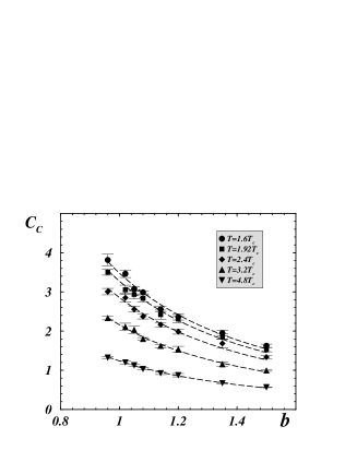
Figure 3: The pre-Coulomb coupling $C_{C}$ and the fits of $C_{C}$ by eq. (71) for various temperatures $T$.

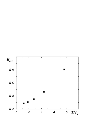
Figure 4: The product of the screening length and the continuum monopole density, eq. (68), calculated from the lattice monopole action (in units of the string tension).

The lattice Coulomb form of the action and proportionality of the pre-Coulomb term to $b^{-2}$ at large values of $b$ was established [21] also in the three-dimensional Georgi-Glashow model for the ’t Hooft-Polyakov monopoles. These facts does not come unexpected from the point of view of the discussion above.

3.3 Lattice monopole density

As we have seen from previous section the density of squared lattice monopole charge should also contain the information about the parameters of the Coulomb gas model. According to eq. (59) the large-$b$ asymptotics of the quantity $\langle k^{2}(b)\rangle/b^{2}$ can be used to extract the product of the screening length and the continuum monopole density $R$, eq. (68). We have measured the density of squared lattice monopole charge for all available temperatures and lattice monopole sizes. As an example we plot in figures 6 and 6 the quantity $\langle k^{2}(b)\rangle/b^{2}$ $vs.$ the lattice monopole size, $b$, for lowest and highest available temperatures, respectively.

Figure 5: The ratio $\langle k^{2}(b)\rangle/b^{2}$ vs. lattice monopole size, $b$, at $T=1.6\,T_{c}$.

Figure 6: The same as in figure 6 but for $T=4.8\,T_{c}$.

Our theoretical expectations (59) indicate that the function $\langle k^{2}(b)\rangle/b^{2}$ must vanish at small monopole sizes and tend to constant at large $b$. This behaviour can be observed in our numerical data, figure 6, up to some jumps for densities with different $n_{s}$. We ascribe these jumps to the lattice artifacts emerged due to finiteness of the fine lattice spacing, $a$, and finite volume effects.

Figure 7: The same quantity as in figure 4 but now calculated from the lattice monopole density.

According to eq. (59) we should know the large-$b$ asymptotics of $\langle k^{2}(b)\rangle/b^{2}$ to get the quantity $R$, eq. (68). These asymptotics are approximated by averaging of the appropriate $n_{s}=8$ data for which the behaviour of the function in question is almost flat. Then we get the product of the screening length and the continuum monopole density, $R$, depicted in figure 7.

The result is very similar to the one obtained from the behavior of the lattice monopole action. However, the quantity $R$ obtained from the lattice monopole density is a bit larger than the same quantity calculated from the lattice monopole action. This fact can be expected since we have approximated the asymptotics of $\langle k^{2}(b)\rangle/b^{2}$ by the average of the $n_{s}=8$ data which may slightly differ from a correct asymptotics.

3.4 Check of the Coulomb gas picture for continuum monopoles

Although both quantities $R_{\rho}$ and $R_{act}$ correspond to the product of the screening length and the continuum monopole density, from a numerical point of view both $R$’s are independent. To check the self-consistency of our approach we plot the ratio of these quantities in figure 9. It is clearly seen that the ratio is independent of the temperature and very close to unity, as expected. The 10%–15% deviation of this quantity from unity may be explained by reasons mentioned in the end of the previous subsection.

Figure 8: Check of the self-consistency: the ratio of the quantities $R$, eq. (68) obtained from the lattice monopole action and density.

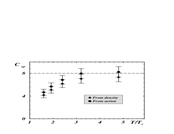
Figure 9: Check of the dilute Coulomb gas picture: quantities $C_{sp}$, eq. (72), calculated from the action and density.

A check of the validity of the Coulomb gas picture can be obtained with the help of the quantity

$$C_{sp}(T)=\frac{\sigma_{sp}(T)}{\lambda_{D}(T)\,\rho(T)}\equiv\frac{\sigma_{sp}(T)}{R(T)}\,,$$ (72)

where $\sigma_{sp}$ is the spatial string tension. In the abelian projection approach the spatial string tension should be saturated by the contributions from the static continuum monopoles. In the dilute Coulomb gas of monopoles the string tension is [18]: $\sigma=8\sqrt{\rho}/g_{M}$ while the screening length is given by (5). These relations imply that in the dilute Coulomb gas of continuum monopoles we should get $C_{sp}=8$.

We use the results for the spatial string tension of ref. [22] in the high temperature $\mathop{\rm SU}\nolimits(2)$ gluodynamics. It was found that for the temperatures higher than $T\approx 2T_{c}$ the spatial string tension can be well described by the formula: $\sigma_{sp}(T)=0.136(11)\,g^{4}_{4D}(T)\,T^{2}$, where $g_{4D}(T)$ is the four-dimensional $\mathop{\rm SU}\nolimits(2)$ 2-loop running coupling constant,

$$g^{-2}_{4D}(T)=\frac{11}{12\,\pi^{2}}\log\left(\frac{T}{\Lambda_{T}}\right)+\frac{17}{44\,\pi^{2}}\log\left[2\log\Bigl{(}\frac{T}{\Lambda_{T}}\Bigr{)}\right],$$

with the scale parameter $\Lambda_{T}=0.076(13)\,T_{c}$. Taking also into account the relation between the critical temperature and the zero-temperature string tension [23], $T_{c}=0.69(2)\,\sqrt{\sigma}$ we calculate the quantity $C_{sp}$ and plot it in figure 9 as a function of the temperature, $T$. If the Coulomb picture works then $C_{sp}$ should be close to $8$. From figure 9 we conclude that this is indeed the case at sufficiently high temperatures, $T/T_{c}\gtrsim 2.5$.

4 Conclusions

In order to describe the lattice monopole dynamics we have proposed to consider the lattice monopoles as the defects which are blocked from continuum. In other words the lattice was suggested to be a measuring device for the continuum monopoles. As a result we are able to draw the following conclusions:

• Using the Monte Carlo results for the density of the squared monopole charges and the monopole action we are able to calculate the product of the abelian magnetic screening length and the monopole density corresponding to the continuum Coulomb gas model. The values of this parameter obtained from density and action measurements are consistent with each other and — at sufficiently high temperatures — are consistent with known results for the spatial string tension. At temperatures $T/T_{c}\gtrsim 2.5$ the spatial string tension is dominated by contributions from the continuum static monopoles.

• The continuum Coulomb gas model can describe the results of the Monte Carlo simulations for the action and density of the lattice monopoles. The dependence of these quantities on the physical sizes of the lattice monopoles (the size of the cell which is used for the monopole detection) is in a good agreement with the analytical predictions.

• The lattice monopole action is dominated by the mass and the Coulomb terms for, respectively, small and large sizes of the lattice monopoles. A relation between the density of the squared magnetic charges and the monopole action is established (eqs. (18), (51), (52) and/or eqs. (36), (38), (60)). Our analytical derivation was done in a gaussian approximation. We have shown that the corrections to the leading terms of the action are small in the large-$b$ limit. A detailed analysis of the corrections will be discussed elsewhere [19].

We believe that this method can also be applied to the four dimensional non-abelian gauge theory. We think that this would allow to get (at least, a part of) parameters of the dual superconductor model.

References

-
[1]
G. ’t Hooft, Gauge theories with unified weak, electromagnetic
and strong interactions, in High energy physics, A. Zichichi
ed., EPS International Conference, Palermo 1975;
S. Mandelstam, Vortices and quark confinement in nonabelian gauge theories, Phys. Rept. 23 (1976) 245. - [2] G. ’t Hooft, Topology of the gauge condition and new confinement phases in nonabelian gauge theories, Nucl. Phys. B 190 (1981) 455.
-
[3]
M.N. Chernodub, M.I. Polikarpov and A.I. Veselov, Effective
constraint potential for abelian monopole in lattice
gauge theory, Phys. Lett. B 399 (1997) 267 [hep-lat/9610007];
Monopole order parameter in lattice gauge theory,
Nucl. Phys. 49 (Proc. Suppl.) (1996) 307 [hep-lat/9512030];
A. Di Giacomo and G. Paffuti, A disorder parameter for dual superconductivity in gauge theories, Phys. Rev. D 56 (1997) 6816 [hep-lat/9707003]. -
[4]
T. Suzuki and I. Yotsuyanagi, A possible evidence for abelian
dominance in quark confinement, Phys. Rev. D 42 (1990) 4257;
G.S. Bali, V. Bornyakov, M. Muller-Preussker and K. Schilling, Dual superconductor scenario of confinement: a systematic study of gribov copy effects, Phys. Rev. D 54 (1996) 2863 [hep-lat/9603012]. -
[5]
A.S. Kronfeld, M.L. Laursen, G. Schierholz and U.J. Wiese,
Monopole condensation and color confinement,
Phys. Lett. B 198 (1987) 516;
A.S. Kronfeld, G. Schierholz and U.J. Wiese, Topology and dynamics of the confinement mechanism, Nucl. Phys. B 293 (1987) 461. -
[6]
M.N. Chernodub and M.I. Polikarpov, Abelian projections and
monopoles, in Confinement, duality, and nonperturbative
aspects of QCD, P. van Baal ed., Plenum Press, p. 387,
hep-th/9710205;
R.W. Haymaker, Confinement studies in lattice QCD, Phys. Rept. 315 (1999) 153 [hep-lat/9809094]. -
[7]
S. Ejiri, S.-I. Kitahara, Y. Matsubara and T. Suzuki, String
tension and monopoles in QCD,
Phys. Lett. B 343 (1995) 304 [hep-lat/9407022];
S. Ejiri, Monopoles and spatial string tension in the high temperature phase of QCD, Phys. Lett. B 376 (1996) 163 [hep-lat/9510027]. - [8] P. Giovannangeli and C.P. Korthals Altes, ’t Hooft and Wilson loop ratios in the QCD plasma, Nucl. Phys. B 608 (2001) 203 [hep-ph/0102022].
- [9] T.A. DeGrand and D. Toussaint, Topological excitations and Monte Carlo simulation of abelian gauge theory, Phys. Rev. D 22 (1980) 2478.
- [10] W. Bietenholz and U.J. Wiese, Perfect lattice actions for quarks and gluons, Nucl. Phys. B 464 (1996) 319 [hep-lat/9510026].
- [11] W. Bietenholz, Perfect scalars on the lattice, Int. J. Mod. Phys. A 15 (2000) 3341 [hep-lat/9911015].
- [12] W. Bietenholz and U.J. Wiese, A perturbative construction of lattice chiral fermions, Phys. Lett. B 378 (1996) 222 [hep-lat/9503022].
- [13] W. Bietenholz, R. Brower, S. Chandrasekharan and U.J. Wiese, Perfect lattice topology: the quantum rotor as a test case, Phys. Lett. B 407 (1997) 283 [hep-lat/9704015].
-
[14]
M.N. Chernodub et al., An almost perfect quantum lattice action
for low-energy gluodynamics, Phys. Rev. D 62 (2000) 094506
[hep-lat/0006025];
S. Fujimoto, S. Kato and T. Suzuki, A quantum perfect lattice action for monopoles and strings, Phys. Lett. B 476 (2000) 437 [hep-lat/0002006]. - [15] V.G. Bornyakov et al., Anatomy of the lattice magnetic monopoles, Phys. Lett. B 537 (2002) 291 [hep-lat/0103032].
-
[16]
M.N. Chernodub et al., An almost perfect quantum lattice action
for low-energy gluodynamics, Phys. Rev. D 62 (2000) 094506
[hep-lat/0006025];
M.N. Chernodub, S. Kato, N. Nakamura, M.I. Polikarpov and T. Suzuki, Various representations of infrared effective lattice gluodynamics, hep-lat/9902013;
V. Bornyakov and M. Muller-Preussker, Continuum limit in abelian projected lattice gauge theory, Nucl. Phys. 106 (Proc. Suppl.) (2002) 646 [hep-lat/0110209]. - [17] K. Ishiguro, T. Suzuki and T. Yazawa, Effective monopole action at finite temperature in gluodynamics, J. High Energy Phys. 01 (2002) 038 [hep-lat/0112022].
- [18] A.M. Polyakov, Quark confinement and topology of gauge groups, Nucl. Phys. B 120 (1977) 429.
- [19] M.N. Chernodub, K. Ishiguro, T. Suzuki, in preparation.
- [20] T.L. Ivanenko, A.V. Pochinsky and M.I. Polikarpov, Extended abelian monopoles and confinement in the lattice gauge theory, Phys. Lett. B 252 (1990) 631.
-
[21]
T. Yazawa and T. Suzuki, Lattice instanton action from 3d Georgi-Glashow model, J. High Energy Phys. 04 (2001) 026
[hep-lat/0101004];
T. Suzuki et al., Topics of monopole dynamics in gluodynamics, Nucl. Phys. 106 (Proc. Suppl.) (2002) 631 [hep-lat/0110059]. - [22] G.S. Bali, J. Fingberg, U.M. Heller, F. Karsch and K. Schilling, The spatial string tension in the deconfined phase of the (3+1)-dimensional gauge theory, Phys. Rev. Lett. 71 (1993) 3059 [hep-lat/9306024].
- [23] J. Fingberg, U.M. Heller and F. Karsch, Scaling and asymptotic scaling in the gauge theory, Nucl. Phys. B 392 (1993) 493 [hep-lat/9208012].