Abstract

The Dirac operator describing the coupling of continuum quark fields to $SU(2)$ center vortex world-surfaces composed of elementary squares on a hypercubic lattice is constructed. It is used to evaluate the quenched Dirac spectral density in the random vortex world-surface model, which previously has been shown to quantitatively reproduce both the confinement properties and the topological susceptibility of $SU(2)$ Yang-Mills theory. Under certain conditions on the modeling of the vortex gauge field, a behavior of the quenched chiral condensate as a function of temperature is obtained which is consistent with measurements in $SU(2)$ lattice Yang-Mills theory.

PACS: 12.38.Aw, 12.38.Mh, 12.40.-y

Keywords: Center vortices, infrared effective theory, Dirac spectrum, spontaneous chiral symmetry breaking

1 Introduction

The random vortex surface model [1],[2] is an infrared effective theory which aims to describe the relevant physical fluctuations determining the low-energy nonperturbative sector of the strong interaction. It is based on collective magnetic vortex degrees of freedom [3]-[10] which are represented by closed two-dimensional world-surfaces in four-dimensional (Euclidean) space-time. The chromomagnetic flux carried by the vortices is quantized according to the center of the gauge group. The vortex world-surfaces are treated as random surfaces, an ensemble of which in practice is generated using Monte Carlo methods on a hypercubic lattice; the surfaces are composed of elementary squares (plaquettes) on that lattice. The spacing of the lattice is a fixed physical quantity, related to an intrinsic thickness of the vortex fluxes, and represents the ultraviolet cutoff inherent in any infrared effective framework. This model can be adjusted such as to quantitatively reproduce the confinement properties of $SU(2)$ lattice gauge theory [1], including the finite-temperature transition to the deconfined phase. It simultaneously predicts a quantitatively correct topological susceptibility, again as a function of temperature [2]. The properties of the model vortices closely parallel the ones obtained for vortex configurations extracted from the full $SU(2)$ lattice Yang-Mills ensemble using an appropriate gauge fixing and projection procedure [8],[9], cf. [11]-[14].

The aim of the present work is to investigate whether also the third central nonperturbative phenomenon determining low-energy strong interaction physics, namely the spontaneous breaking of chiral symmetry, can be correctly described within the random vortex surface model. For this purpose, a number of technical developments are carried out. The coupling of the gluonic vortex degrees of freedom to (continuum) quark fields is governed by the Dirac operator; in order to construct this operator, an explicit representation of vortex configurations in terms of continuum gauge fields is needed. Having specified such a representation, matrix elements of the Dirac operator can be calculated in a truncated infrared quark basis. Via the (ensemble-averaged) spectral distribution of the resulting Dirac matrix, which is obtained numerically, the (quenched) chiral condensate is extracted; this condensate can be used as an order parameter for spontaneous chiral symmetry breaking. Under certain conditions on the explicit vortex gauge field modeling, the chiral condensate as a function of temperature behaves in a manner consistent with $SU(2)$ lattice gauge theory.

To date, several explorations of spontaneous chiral symmetry breaking within the vortex picture have been presented. One of these lines of investigation [15]-[17] deals with the vortex configurations extracted from the full $SU(2)$ lattice Yang-Mills ensemble by gauge fixing and projection [8],[9]. Removing these vortices from $SU(2)$ lattice configurations leads to the restoration of chiral symmetry [15]; on the other hand, the extracted vortices by themselves break chiral symmetry at zero temperature [16]. In the chiral limit, a divergence of the chiral condensate is observed which is reminiscent of the behavior detected in full $SU(2)$ Yang-Mills theory using domain-wall fermions [18]; such a divergence will also be observed in the Dirac spectra obtained in the present work, cf. section 5. Crossing into the deconfined regime, chiral symmetry remains broken, to an extent which differs qualitatively [17] from the breaking found in the aforementioned domain-wall fermion calculations. In view of this result, the significance of the chiral condensate induced by vortices and its relation to the condensate obtained in full Yang-Mills theory remained in doubt. In the present work, the behavior of the chiral condensate in the high-temperature regime will turn out to depend strongly on the modeling of the vortex gauge field. Only a sufficiently smooth definition of the gauge field yields a behavior of the chiral condensate consistent with full Yang-Mills theory. Possibly the vortex extraction procedure used in [17] endows the vortices with excessive spurious ultraviolet disorder which leads to the unnatural result for the chiral condensate in the deconfined phase.

On the other hand, quite recently an effective vortex model (in the guise of a $Z(2)$ gauge theory in the strong coupling limit) was considered [19] which to a certain extent follows the logic of the random vortex surface model investigated here. At the expense of a more limited scope of applicability (the ultraviolet cutoff is e.g. too low to permit a description of the deconfinement phase transition), the dynamics is simplified to the point where analytical estimates of the chiral condensate become possible. These estimates appear to be close to phenomenologically accepted values for the unquenched, dynamical quark case. However, the extreme limit considered seems rather artificial in that the quenched and the dynamical quark cases yield comparable chiral condensates. Presumably, since one possibility of arriving at estimates of the type used in [19] appears to lie in invoking the large-$N_{c}$ expansion ($N_{c}$ denoting the number of colors), this should not come as a surprise; the large-$N_{c}$ expansion is by construction quenched to leading order, dynamical quark effects only entering subdominant terms. By contrast, the quenched chiral condensate obtained in lattice Yang-Mills theory [20] exceeds the one expected phenomenologically in the presence of dynamical quarks by about an order of magnitude; clearly, the quark determinant weighting of the dynamical quark ensemble must be viewed as one of the dominant physical effects in order to reconcile the quenched approximation with the dynamical quark case. In view of this, the meaning of the chiral condensate discussed in [19] remains unclear, as does the question whether the quoted values in fact support or weaken the basis for that model.

2 General remarks on the formulation of a vortex gauge field model

In the applications of the random vortex surface model hitherto considered [1],[2], it was not necessary to explicitly construct a gauge field associated the vortex configurations arising in the model. To evaluate confinement properties, encoded in Wilson loops [1], it is sufficient to specify the space-time location of the vortex world-surfaces; to evaluate the topological charge [2], it is sufficient to specify the vortex field strength, which is localized on those surfaces. By contrast, construction of the Dirac operator implies specifying the gauge field itself. The freedom inherent in this specification entails ambiguities due to the fact that the concept of an infrared effective model of gauge and quark fields to a certain extent clashes with gauge invariance; after all, the distinction whether a given configuration is infrared or not is a gauge-dependent one. In an infrared effective model of gauge and quark fields, manifest gauge invariance can only be sustained with respect to gauge transformations $U$ which are themselves infrared. Specifically, when using a truncated basis of quark wave functions (as will be done in this investigation), invariance under a change of the gauge in which the gauge field ensemble is given is only guaranteed to the extent that, for a quark wave function $q$ represented in the aforementioned basis, also $Uq$ can be represented to good accuracy in that basis. Conceptually, this is not an obstacle to model-building; it just implies that a full specification of the model must include a fixed choice of gauge, and that predictive power is curtailed to the extent that observables depend on the precise gauge field modeling. In general, some observables have to be used to fix the model before additional ones can be predicted.

Ideally, the most consistent gauge field description of a given vortex field strength ensemble would be one in which the gauge field is itself as smooth, i.e. infrared, as possible, such as the Landau gauge. In practice, the choice is constrained by considerations of technical manageability, and also by certain idealizations of the vortex configurations which already occur on the level of the field strengths, cf. below. In order to obtain information about the dependence of observables on the construction of the gauge field, in this work different choices will be explored, which, configuration by configuration, describe the same vortex world-surfaces, but are related by gauge transformations which by no means are infrared. It will turn out that chiral symmetry breaking in the confined phase is quite robust as the modeling of the gauge field is changed; on the other hand, the Dirac spectrum in the deconfined, high temperature phase exhibits a substantial dependence on the gauge field modeling - gratifyingly, the most consistent (smoothest) construction turns out to best reproduce the results of full Yang-Mills measurements.

Before proceeding to present the construction of the gauge field in detail, a few remarks are in order concerning the idealizations of the vortex field strengths mentioned further above, which were already introduced in previous considerations of the random vortex surface model. The vortices hitherto used to evaluate observables within the model were idealized in two ways: For one, vortex fluxes were taken to be infinitely thin, i.e. the associated world-surfaces are truly two-dimensional, with no transverse thickness in the remaining two space-time directions. Note that this idealization is gauge-invariant; it is a statement about the structure of the modulus of the field strength tr$\,F^{2}$. On the other hand, as a vector in color space, the field strength $F$ on vortex surfaces was taken to point exclusively into the positive or the negative 3-direction; generic vortex surfaces are non-oriented, i.e. consist of patches of alternating orientation. Note that the color direction of $F$ can be changed by gauge transformations; thus, the configurations hitherto used can be viewed as having been specified in a gauge of the maximally Abelian type.

It should be emphasized that these are the properties of the field strengths used to evaluate observables within the model. By contrast, in the generation of the vortex surface ensemble, a physical thickness of the vortices is indeed implicit [1]: A finite action density is associated with vortex surface area and curvature; infinitely thin vortex fluxes of course formally would carry divergent tr$\,F^{2}$. Also, vortex surfaces cannot be packed arbitrarily densely within the model; instead, there is a fixed ultraviolet cutoff, interpreted as a consequence of the vortex thickness. The construction and interpretation of the vortex dynamics is discussed at length in [1].

The idealized thin vortex configurations described above are, however, entirely sufficient for an unambiguous evaluation of the observables considered to date. Neither the asymptotic string tension [1],[22] nor the topological charge [2],[23]-[25] depend on any assumption about the transverse structure of the vortex fluxes, i.e. whether they are thickened or not. Also, both observables are virtually independent of assumptions about the color orientation of the vortex field strength. For the topological charge, this is somewhat less obvious than for the Wilson loop; this issue is discussed in detail in [2].

On the other hand, in the case of the Dirac operator spectrum to be discussed here, the issue is a priori not as clear-cut; it is therefore necessary to be specific about how the aforementioned idealizations will be dealt with. In the following treatment, the idealization of thinness of vortex flux will be maintained; a sufficiently simple and manageable construction of manifestly thick vortex fluxes did not become apparent in the course of this investigation. Instead, a model assumption will be used which is familiar e.g. from the Nambu–Jona-Lasinio (NJL) quark model. Namely, as already hinted at above, the quark modes will be subject to a fixed ultraviolet cutoff, the same one which is implicit in the model vortex dynamics via the spacing of the lattice on which the vortex surfaces are defined [1]. In the NJL model, the quark current-current interaction formally is point-like; however, the ultraviolet cutoff on the quark modes effectively smears out the four-quark vertex into a nonlocal interaction. In complete analogy, within the present treatment, the interaction between a quark and a vortex formally takes place on an infinitely thin submanifold (to be specific, a three-dimensional volume, the two-dimensional boundary of which precisely gives the location of the vortex field strength, cf. section 3.1). However, the ultraviolet cutoff on the quark modes will effectively smear this out in the direction perpendicular to the volume (and, at its boundary, in the two directions perpendicular to the idealized thin vortex field strength). Thus, the thickening of the vortices is not carried out explicitly in the vortex gauge fields, but is effectively accomplished by smearing out the vortex-quark vertex via the ultraviolet cutoff on the quark fields.

Turning to the issue of the color orientation of the vortex field strength, a more sophisticated approach will be pursued, for the following reason. If one works with a globally defined field strength, pointing either into the positive or the negative 3-direction in color space, and one attempts to globally define an Abelian gauge field generating this field strength, then, in the (generic) case of nonorientable vortex surfaces, one necessarily introduces Dirac string world-surfaces into the description, emanating from the lines on the vortex surfaces at which the orientation switches. After all, a globally defined (Abelian) gauge field must satisfy continuity of (Abelian) magnetic flux. This would not constitute a problem if one worked with a complete quark basis, i.e. solved the Dirac equation exactly. Then, the quark wave functions would exhibit singularities along the Dirac strings which would serve to cancel any physical effect of these strings, i.e. the Dirac strings would be unobservable, as they should be. However, in any truncated calculation such as will be pursued here, the cancellation would not be perfect; instead, the Dirac strings effectively would act as additional physical magnetic fluxes (of double magnitude compared with vortex fluxes) with which the quarks can interact. Thus, more magnetic disorder would be effectively present than the model aims to describe.

The way out of this dilemma lies in instead using a Wu-Yang construction of the gauge field [21]. In other words, the gauge field will be defined on local patches, which are then related to one another via transition functions on their overlaps; the transition functions in general will have to be non-Abelian. The patches should be chosen sufficiently small, such that, on any given patch, the vortex surfaces can be oriented; in this case, no Dirac strings arise in the associated Abelian gauge field, which is then well-defined on the whole patch. The reader should however be forewarned that constraints on the space-time form of the transition functions in generic vortex configurations will force the reintroduction of some spurious fluxes (via additional non-Abelian gauge field components) which are formally similar to Dirac strings, but with the crucial difference that they manifestly decouple from the smooth infrared quark fields. Thus, spurious fluxes are not completely eliminated by the construction presented below; rather, they are recast in an innocuous form. In practice, the Dirac equation will be solved using the finite element method, i.e. using a basis of localized quark wave functions. Thus, it is natural (and sufficient) to use the supports of the individual basis functions, i.e. the finite elements, as the space-time patches on which the gauge field is locally defined. Specifics on these finite elements follow further below.

3 Construction of the vortex gauge field

3.1 Local structure of the gauge field

A closed $SU(2)$ vortex world-surface $S$ along with its quantized chromomagnetic flux can, to a large extent, be characterized by the gauge-invariant property

$$W[C]=(-1)^{L(C,S)}$$ (1)

for any Wilson loop $W[C]$ linked $L(C,S)$ times to the surface $S$. Note that the factor $(-1)$ on the right hand side of eq. (1) corresponds to the only nontrivial center element of the $SU(2)$ group, which will be the subject of investigation in the following. It is in this sense that vortex flux is quantized according to the center of the gauge group. For higher $SU(N)$ groups, the $(-1)$ on the right hand side of eq. (1) is replaced by center elements of those groups. In general, there are several such center elements and, consequently, several types of quantized vortex flux.

For the purpose of constructing a gauge field encoding the property (1), it is useful to shift the emphasis of the description [23], namely from the closed surfaces $S$ to three-dimensional volumes $\Sigma$ bounded by $S$, i.e. $S=\partial\Sigma$. Then (1) can be rewritten as

$$W[C]=(-1)^{I(C,\Sigma)}$$ (2)

in terms of the intersection number $I(C,\Sigma)$ of $C$ with $\Sigma$.

The random vortex surface model studied here is formulated on a space-time lattice, on which vortex surfaces are composed of elementary squares; correspondingly, the volumes $\Sigma$ are composed of elementary three-dimensional cubes. To specify a volume $\Sigma$, as yet without orientation, it is sufficient to associate each elementary three-dimensional cube $K$ on the lattice with a value $\phi(K)=\pm 1$, $\phi(K)=1$ signifying that $K$ is not part of $\Sigma$, and $\phi(K)=-1$ signifying that it is. The question of how a volume $\Sigma$ for a given vortex surface $S$ can be obtained in practice will be discussed further below; for the time being, let it be assumed that such a volume has been found (obviously there is some freedom in choosing $\Sigma$, since it merely must satisfy $\partial\Sigma=S$). The Wilson loop (2) in this language becomes

$$W[C]=\prod_{i:\,K_{i}\cap C\neq 0}\phi(K_{i})$$ (3)

where the product is taken over all cubes $K_{i}$ intersected by $C$.

This must now be translated into the gauge field $A(K)$ associated with each cube $K$, i.e. a gauge field must be constructed which satisfies

$$\exp\left(i\int_{P}dx_{\mu}A_{\mu}(K)\right)=\phi(K)$$ (4)

for a path $P$ in $\mu$-direction intersecting the three-dimensional cube $K$, assumed here to extend into all directions but the $\mu$-direction. Gauge fields $A_{\mu}(K)$ which reproduce this property can be given as follows. If $K$ is the cube extending from the lattice site $\bar{x}$ into all (positive) directions except the $\mu$-direction, then (with $a$ denoting the lattice spacing and the third Pauli matrix $\sigma^{3}$ encoding the color structure)

$$A_{\mu}(K)=n(K)\pi\sigma^{3}\delta(x_{\mu}-\bar{x}_{\mu})\prod_{\lambda\neq\mu}\theta(x_{\lambda}-\bar{x}_{\lambda})\theta(\bar{x}_{\lambda}+a-x_{\lambda})$$ (5)

i.e. $A(K)$ has support only on $K$ and points into the space-time direction perpendicular to $K$; furthermore, its strength depends on an integer $n(K)$ which, at this point, is merely constrained to satisfy

$$\exp(i\pi n(K))=\phi(K)\ ,$$ (6)

i.e. $n(K)$ must be even for $\phi(K)=1$ and odd for $\phi(K)=-1$. Apart from this, the integer $n(K)$ still remains to be specified (which is where the orientation of $\Sigma$ will attain relevance, along with the necessity of dividing space-time into patches, as already indicated in section 2). Finally, the color structure of the gauge field is given by the third Pauli matrix $\sigma^{3}$ in (5). As already discussed in section 2, this is a specification which was already adopted previously [2],[23] on the level of the vortex field strengths; it implies that vortex configurations at this stage are cast in a gauge of the maximally Abelian type. Another strong restriction of the gauge freedom is of course implied by the space-time form of (5); the gauge field only has support on a three-dimensional submanifold made up of elementary three-dimensional cubes in the lattice, as already indicated and discussed in section 2. In fact, apart from the integer $n(K)$ to be specified in (5), the only freedom which remains is the choice of the three-dimensional volume $\Sigma$ spanning the given vortex surface $S$. This freedom corresponds to the $Z(2)$ part of the $SU(2)$ gauge freedom of $SU(2)$ Yang-Mills theory [23]. Again, the question of how $\Sigma$ can be obtained for a given vortex surface $S$ in practice is deferred for now; suffice it to state that more than one choice will be explored below.

3.2 Global topology and space-time patches

In a gauge field formulation of vortex configurations, one needs a more specific characterization of vortices than is contained in the property (1); this formally manifests itself in the a priori freedom in the choice of the integer $n(K)$ in (5). Within the random vortex surface model, the only physical degrees of freedom are elementary vortex fluxes whose gauge field description satisfies

$$\oint_{C}dx_{\mu}A_{\mu}=\pm\pi\sigma^{3}$$ (7)

for a line integral along an infinitesimal loop $C$ circumscribing the vortex.

This property will serve to fix the integer $n(K)$ in (5) to a large extent. Eq. (7) should be contrasted with the exponentiated form (1), which would allow any odd integer multiple on the right hand side of (7). It should be noted that the specification (7) was already used when calculating the topological charge of vortex configurations [2],[23]; fluxes corresponding to integer multiples of (7) of course carry associated multiple field strengths, which would enter the topological density $\epsilon_{\mu\nu\kappa\lambda}F_{\mu\nu}F_{\kappa\lambda}$. Such multiple field strengths were not allowed for in [2],[23]; the requirement (7) thus is not a new feature of the present investigation. The only freedom in (7) is the choice of sign, i.e. the orientation of the vortex flux; this can be seen as a vestige of the color rotation freedom present in the characterization (1) which still remains after fixing the color direction of the gauge field via the Pauli matrix $\sigma^{3}$ in (7). In view of the nonorientability of generic vortex surfaces [13], this residual freedom will be crucial.

This leads to a central issue, namely how the different individual cubes $K_{i}$ are sewn together at the elementary squares (plaquettes) they share. By applying the specification (7) to a small loop encircling each plaquette on the lattice, a set of constraints on the choices of integers $n(K_{i})$, cf. eq. (5), can be derived. To be precise, if the plaquette $p$ extends from the lattice site $\bar{x}$ into the positive $\mu$ and $\nu$ directions, and $\lambda,\kappa$ denote the other two space-time directions, then consider the square loop $C(p)$ given by the following sequence of corners,

$$C(p):\ \ \bar{y}\ \ \longrightarrow\ \ \bar{y}+ae_{\lambda}\ \ \longrightarrow\ \ \bar{y}+ae_{\lambda}+ae_{\kappa}\ \ \longrightarrow\ \ \bar{y}+ae_{\kappa}\ \ \longrightarrow\ \ \bar{y}$$

starting and ending at $\bar{y}=\bar{x}+(a/2)(e_{\mu}+e_{\nu}-e_{\lambda}-e_{\kappa})$, where $a$ denotes the lattice spacing and $e_{\rho}$ the unit vector in the $\rho$-direction. Clearly, (7) then implies a constraint on the four cubes $K_{i}$ whose boundaries contain the plaquette $p$ (and which are thus intersected by $C(p)$), namely

$$\!\!\!\!\!\!\!\!\oint_{C(p)}dx_{\mu}A_{\mu}=$$

$$\ \ \ \ \ =\left[n(K_{\lambda}(\bar{x}-ae_{\kappa}))+n(K_{\kappa}(\bar{x}))-n(K_{\lambda}(\bar{x}))-n(K_{\kappa}(\bar{x}-ae_{\lambda}))\right]\pi\sigma^{3}$$

$$\ \ \ \ \ \in\ \ \{0,\pm\pi\sigma^{3}\}$$ (8)

where $K_{\rho}(\bar{x})$ denotes the cube extending from $\bar{x}$ into all (positive) directions but the $\rho$ direction. In physical terms, the plaquette $p$ should carry at most one single unit of vortex flux (of either orientation). Every plaquette on the lattice generates one such constraint. It should be noted that this does not exclude any particular cube $K$ on its own carrying an arbitrary integer $n(K)$ in eq. (5); only from the point of view of choosing a gauge in which the gauge fields are as “smooth” as possible, cf. the general discussion in section 2, it is desirable to keep the magnitude of $n(K)$ as small as can be achieved; how small this is in practice will be commented upon below.

With the constraints (8) relating neighboring cubes $K_{i}$ on the lattice, the global topology of the volumes $\Sigma$ made up of such cubes enters the description. Namely, generic vortex surfaces $S$, and, concomitantly, volumes $\Sigma$ spanning $S$, are not orientable [13]. Formally, this expresses itself in the property that the constraints (8) cannot all be simultaneously satisfied throughout space-time with a unique choice $n(K_{i})$ for all cubes $K_{i}$ in the lattice. Rather, for non-orientable $\Sigma$, it is unavoidable to encounter frustrations in the attempt to satisfy all the constraints, i.e. one will find some plaquettes $p$ within the volume $\Sigma$ which yield the value

$$\oint_{C(p)}dx_{\mu}A_{\mu}=\pm 2\pi\sigma^{3}\ ,$$ (9)

thus carrying flux double that of a vortex, cf. Fig. 1 (left). Not being intended to appear as physical flux degrees of freedom within the random vortex surface model, these are the Dirac string world-surfaces which are unavoidable in a global, uniquely defined Abelian gauge field describing a non-oriented vortex surface; their boundaries correspond to monopole loops on the vortex sheets [23]. It is clear that such Dirac strings must arise when the vortex surface $S$ is not orientable: In that case, there must be lines on the vortex surface where flux orientation changes (the monopoles), and a globally defined Abelian gauge field, which satisfies continuity of flux, must therefore contain Dirac strings supplying the change in vortex flux at the monopoles.

Figure 1: Nonoriented gauge field support volume $\Sigma$ in a two-dimensional slice of space-time. In such a slice, vortices show up as the solid points, volumes $\Sigma$ emanating from them as the solid lines. The directions of the vortex fluxes at the boundaries of $\Sigma$, fixed a priori, here happen to be such that the segments of $\Sigma$ emanating from the different vortices are forced to have mutually incompatible orientation. This is indicated by the arrows, which symbolize (directed) line integrals $\int A_{\mu}dx_{\mu}$; all of the line integrals indicated in the figures yield the same value, for definiteness $+\pi\sigma^{3}$. Left: Attempt at a global definition of the gauge field; the volume $\Sigma$ then necessarily contains the indicated Dirac string, satisfying the property (9). Right: Wu-Yang construction, with space-time subdivided into two patches, on each of which the volume $\Sigma$ is oriented. Gauge fields on the two patches are related by the transition function $U$. In the simple example depicted here, $U$ can be chosen constant in the whole overlap region shared by the two patches. In generic configurations, the presence of other vortices nearby forces the space-time region of nontrivial $U$ to be more localized, namely onto the immediate vicinity of $\Sigma$. This is discussed in more detail further below.

For reasons motivated in section 2, such (Abelian) Dirac strings are to be excluded from the gauge field in the present framework. Instead, the Wu-Yang construction will be used: Define the gauge field only locally on patches, sufficiently small such that all constraints (8) arising in any particular patch can be simultaneously satisfied. The different patches are then related via transition functions, cf. Fig. 1 (right). The precise construction is as follows. The patches are the interiors of all the $(2a)^{4}$ hypercubes centered on the sites of the lattice, $a$ denoting the lattice spacing. This is a natural choice, since these hypercubes will at the same time be the supports of the quark basis functions (finite elements) used in the construction of the Dirac operator matrix further below. In practice, these patches are sufficiently small to allow all the constraints (8) (and, of course, (6)) arising on them to be satisfied. In order to achieve this, it furthermore turns out to be sufficient to allow for the values $-2\leq n(K)\leq 2$ in (5). An actual viable choice of $n(K_{i})$ for each of the $32$ cubes $K_{i}$ in a given patch is found by trial and error, starting from an initial cube, assigning values to neighboring cubes such as to satisfy the corresponding constraints (6),(8), and repeating until integers $n(K_{i})$ have been assigned to all cubes (note that the choice is in general not unique). In practice, this procedure uses an insignificant amount of computer time compared with the subsequent treatment of the Dirac matrix; thus, it is not necessary to invent more intelligent strategies for finding a viable set of integers $n(K_{i})$.

3.3 Matching patches - transition functions

To facilitate a simple connection of the different patches via transition functions, two modifications of the gauge field on each patch are still necessary. For one, as already hinted at above, any cube $K$ which is associated with the value $|n(K)|=2$ in at least one of the patches containing it is replaced by two cubes $K_{1}$ and $K_{2}$ parallel to $K$, and displaced from $K$ by a small distance in the direction perpendicular to the cubes, cf. Fig. 2. The new cubes are assigned values $n(K_{1})$, $n(K_{2})$ in all patches containing $K_{1}$ and $K_{2}$ as follows:

$$n(K)=2 \Longrightarrow n(K_{1})=1,\ n(K_{2})=1$$

$$n(K)=-2 \Longrightarrow n(K_{1})=-1,\ n(K_{2})=-1$$ (10)

$$n(K)=0 \Longrightarrow n(K_{1})=1,\ n(K_{2})=-1$$

Clearly, the new gauge field on the two cubes $K_{1}$ and $K_{2}$ fulfils the constraint (7) defining vortex flux just like the original gauge field defined on $K$. All that has happened is that the phase picked up by any line integral intersecting $K$ has been distributed onto the two cubes $K_{1}$ and $K_{2}$ which are slightly displaced from $K$. In effect, the splitting of $K$ corresponds to a deformation of the volume $\Sigma$ spanning the vortex world-surfaces $S=\partial\Sigma$. The original $\Sigma$ is augmented by closed volumes; such an operation does not change $\partial\Sigma$, i.e. the physical content of the vortex configuration. Rather, it implies a ($Z(2)$) change of the gauge in which the gauge field is cast. As a result of the assignment (10), only the values $-1\leq n(K)\leq 1$ are still possible, at the expense of having introduced additional cubes $K$ into the gauge field configurations.

Figure 2: Splitting of a cube $K$ carrying $n(K)=2$ into two parallel cubes $K_{1}$ and $K_{2}$ carrying $n(K_{1})=n(K_{2})=1$.

The second change in the gauge field configurations which is still necessary stems from the following difficulty: In generic vortex configurations, one does not have the freedom to choose constant transition functions throughout the overlaps between different patches, such as in Fig. 1 (right). Instead, the presence of other vortices nearby forces one to localize the nontrivial parts of the transition functions to the immediate vicinities of the cubes $K$ being rotated; in other words, the construction should be local to such an extent that the transition function can be specified independently for each cube $K$, cf. Fig. 3. However, such more sophisticated transition functions are space-time dependent and thus call for additional auxiliary gauge fields in some of the participating patches due to the inhomogeneous term in the gauge transformation law. Specifically, the modification consists in adding a pure gauge as follows. For any cube $K$ associated with the value $n(K)=-1$ on a given patch, consider a space-time region ${\cal E}(K)$ in that patch, bounded by two cubes $K_{+}$ and $K_{-}$ which are parallel to $K$, and which are displaced from $K$ by a small distance $\epsilon$, as well as a small volume $K_{0}$ (of extension $\epsilon$ in one of its directions) connecting $K_{+}$ and $K_{-}$, such as depicted in Fig. 3. Note that any definition of ${\cal E}(K)$ such that ${\cal E}(K)$ contains $K$, but no points more distant from $K$ than $\epsilon$, serves the purpose of the present construction. If desired, it is quite admissible to deform $K_{0}$ in a way which excludes from ${\cal E}(K)$ some points which are closer to $K$ than $\epsilon$. Note also that the distance $\epsilon$ is intended to be even smaller than the distance between two cubes $K_{1}$ and $K_{2}$ used in the cube-splitting procedure discussed in the previous paragraph. Consider furthermore the gauge transformation

$$U_{{\cal E}(K)}(x)=\left\{\begin{array}[]{lcr}1&\mbox{for}&x\notin{\cal E}(K)\\ -i\sigma^{2}&\mbox{for}&x\in{\cal E}(K)\end{array}\right.$$ (11)

and the gauge field $\bar{a}(K)=iU_{{\cal E}(K)}^{\dagger}\partial U_{{\cal E}(K)}$ induced by $U_{{\cal E}(K)}$, which has support on the boundary of ${\cal E}(K)$ described above.

Figure 3: Space-time patch with three cubes $K$, $K_{A}$ and $K_{B}$ which are part of the gauge field support volume $\Sigma$; in the two-dimensional slice displayed, these cubes show up as the solid lines. For definiteness, $n(K_{A})=n(K_{B})=1$ and $n(K)=-1$; there is a vortex at the center of the patch. On a neighboring patch which also contains $K$, this cube shall carry the value $n^{\prime}(K)=1$. The region on which the associated transition function $U$ is nontrivial is localized as specified in the figure; this simultaneously implies supplementing the gauge field in the depicted patch with an auxiliary field $\bar{a}=iU^{\dagger}\partial U$, see text. The field $\bar{a}$ has support on the volumes $K_{+}$, $K_{-}$ and $K_{0}$, which is where $U$ changes as a function of space-time. In general, it cannot be avoided that $K_{0}$ intersects parts of $\Sigma$ (in the absence of $K_{A}$ and $K_{B}$, one could still deform $K_{0}$ such as to circumscribe $K$). Such intersections imply spurious fluxes, see text.

On any patch on which $n(K)=-1$, the field $\bar{a}$ is added to the gauge field in that patch, i.e.

$$A(K)\longrightarrow\left\{\begin{array}[]{lll}A(K)&\mbox{for}&n(K)=1\\ A(K)+\bar{a}(K)&\mbox{for}&n(K)=-1\end{array}\right.$$ (12)

for each cube $K$ in all patches. This modification does not change any Wilson loops nor any line integrals (7) taken in the configuration; also the physically relevant field strength content of the gauge field on the patch in question is not changed, apart from the following subtlety: In general, it is not excluded that $K_{0}$ may be forced to intersect the volume $\Sigma$ which spans the vortex world-surfaces $S=\partial\Sigma$, and which supports a nontrivial gauge field $A$, cf. Fig. 3. In this case, a spurious flux is generated on the intersection surface through the commutator term in the field strength, $F_{\mu\nu}\propto[A_{\mu},\bar{a}_{\nu}]$. Thus, in some cases, spurious fluxes of the Dirac string type are reintroduced; however, the crucial point is that these fluxes have now been cast in a form in which infrared quark propagation manifestly is not influenced by them. Namely, consider any coupling matrix element

$$\int d^{4}x\,q_{1}^{\dagger}\,\bar{a}\,q_{2}$$ (13)

taken between smooth quark wave functions $q_{1}$ and $q_{2}$. Such an integral is negligible, since the fields on $K_{+}$ and $K_{-}$ differ precisely by a sign, and $K_{+}$ and $K_{-}$ are located only a very small distance $\epsilon$ apart; furthermore, the contribution from $K_{0}$ is of order $\epsilon$ due to the small extension of $K_{0}$ in one of its space-time directions. Thus, the smooth quark modes of an infrared effective theory are insensitive to the supplementary field $\bar{a}$. It is not excluded that a more sophisticated construction exists which avoids the residual spurious field strengths induced by the additional presence of $\bar{a}$ altogether; however, in view of the insensitivity of infrared quark propagation with respect to $\bar{a}$, it does not appear necessary to develop such a construction at this stage. In a sense, the situation is opposite to the case of the Dirac string fluxes which one would obtain by naively defining a global Abelian gauge field such as discussed further above; in that case, the fact that one is working with a truncated quark basis precludes the solutions of the Dirac equation adjusting such as to make the Dirac strings invisible. In the present case, it is precisely the infrared sector of smooth quark wave functions which manifestly decouples from any residual spurious fluxes introduced by the addition of the field $\bar{a}$. Note, however, that this is one of the main points preventing a straightforward generalization of the present gauge field definition to explicitly thickened vortex fluxes and gauge field volumes. Such a generalization would entail finite $\epsilon$, and as a consequence, the spurious additional field strengths induced by adding the field $\bar{a}$ as discussed here could no longer be argued to decouple. Thus, a more sophisticated construction of the gauge fields on each patch and the associated transition functions would need to be specified.

Note furthermore that, at this point, one still has a certain amount of freedom as regards the global definition of the gauge field, which will be discussed in more detail below in section 3.4. In particular, it is still possible to vary the space-time density of nontrivial matchings between neighboring patches, i.e. nontrivial transition functions. Comparing the results obtained with constructions which mutually differ in this respect will give an indication of the influence of the rough disorder in the gauge field associated with the presence of those nontrivial transition functions.

Having prepared the gauge field configurations on each space-time patch as described above, it is straightforward to give the corresponding transition functions between patches. Consider two patches, distinguished in the following by denoting all quantities in one patch with a prime and their counterparts in the other patch without a prime. Consider furthermore the space-time region in which the two patches overlap and the set of cubes $K_{i}$ located there, associated with values $n(K_{i})$ and $n^{\prime}(K_{i})$ in the two patches. The associated transition function in that overlap region then is

$$U=\prod_{K_{i}}U^{[n(K_{i})-n^{\prime}(K_{i})]/2}_{{\cal E}(K_{i})}$$ (14)

with $U_{{\cal E}(K)}$ given by (11), i.e. the gauge fields $A$ (including, if present, the auxiliary field $\bar{a}$) and the quark fields $q$ in the two patches are related by

$$A^{\prime} = UAU^{\dagger}-iU\partial U^{\dagger}$$ (15)

$$q^{\prime} = Uq$$ (16)

3.4 Options in the gauge field construction

The gauge field construction presented above still allows for different model options in two respects. In the numerical work further below, a variety of these options will be explored in order to be able to appreciate the dependence of the results on the gauge field modeling, which, after all, contains a range of ambiguities and idealizations as presented in the preceding sections.

One of the options one still has lies in the choice of the volume $\Sigma$ spanning the vortex world-surfaces. A particular such volume $\Sigma$, the construction of which was repeatedly deferred above, can be obtained as follows. As discussed in detail in [1], Monte Carlo updates of vortex configurations in the present model are always carried out simultaneously on all six plaquettes making up the surface of an elementary three-dimensional cube in the lattice; this serves to keep the vortex surfaces closed as they are being updated. As a result, a volume $\Sigma$ whose boundary defines the vortex surfaces can be trivially obtained by keeping track of the cubes being updated. To be precise, if one starts with an empty lattice, $\phi(K_{i})=1$ for all three-dimensional cubes $K_{i}$ in the lattice; whenever an update of (the surface of) a cube $K$ is subsequently accepted, one concomitantly changes $\phi(K)\rightarrow-\phi(K)$. In this way, at any point in the calculation, a viable $\Sigma$, made up of the set of $K_{i}$ with $\phi(K_{i})=-1$, is known.

On the other hand, this is not the only possible $\Sigma$. Instead of working directly with the above $\Sigma$, which will generally be rather random and rough, it is possible to first apply a smoothing algorithm to $\Sigma$. Since the only physically relevant information lies in the boundary of $\Sigma$, it is admissible to add to $\Sigma$, or take away from $\Sigma$, arbitrary closed three-volumes. In practice, this implies sweeping through the lattice, considering each elementary four-cube in turn, and simultaneously updating all eight three-cubes $K_{i}$ making up its boundary, i.e. $\phi(K_{i})\rightarrow-\phi(K_{i})$, whenever this leads to a reduction in the total volume of $\Sigma$. The two options for $\Sigma$ are related by a ($Z(2)$) gauge transformation which however does not vary smoothly in space-time. Consequently, invariance of the Dirac spectrum is not guaranteed in a calculation using a truncated quark basis, as already mentioned in section 2. Thus, the two options represent different possible models which will be explored in the numerical work below; the options will be referred to as “random $\Sigma$” and “smooth $\Sigma$”, respectively. Of course, under the aspect of formulating the gauge field in as smooth a gauge as possible in order to minimize artefacts stemming from rapidly varying gauge transformations, the smooth option seems the preferred one.

The second option one still has in the construction of the gauge field is the following: Above, the gauge field $A$ is initially constructed independently on each space-time patch. As a result, the relative color orientation of adjacent patches, ultimately encoded in the transition functions on the respective overlap regions, is random; there is a high density of overlap regions supporting nontrivial transition functions. However, for any given patch, the transformation $A\rightarrow-A$ leads to an equally admissible gauge field on that patch; this simply corresponds to a gauge transformation $U=-i\sigma^{2}$ constant throughout the patch. Thus, after the initial construction of the gauge field $A$ (but before the addition of the auxiliary gauge field $\bar{a}$ discussed in section 3.3), one has the alternative of performing sweeps through the lattice in which one considers a transformation of the gauge field $A\rightarrow-A$ on each individual patch in turn. Acceptance of such a transformation can be biased such that as many as possible of the resulting transition functions to neighboring patches become trivial. In other words, the transition functions are made maximally smooth. In the language of globally defined gauge fields with monopole and Dirac string singularities, this corresponds to minimizing the space-time density of such singularities. Accordingly, the option of fixing the gauge field orientation at random on the patches will below be referred to as the “random monopole” gauge, whereas the option of maximally smooth transition functions will be referred to as the “minimal monopole” gauge. Note that such an alternative, either choosing the monopoles at random or minimizing their density, was already considered in [2],[14],[26]. The topological susceptibility turned out to be virtually independent of the monopole density, a fact which could be understood in terms of the space-time properties of generic vortex surfaces [2],[14],[26].

4 Vortex-Quark coupling

4.1 Quark basis and Dirac matrix

As already indicated further above, the Dirac equation will be solved using the finite element method. This means that the truncated quark basis is constructed using space-time wave functions $f(x-x_{0})$ associated with, and localized around, each lattice site $x_{0}$ (the Dirac and color structure will be supplemented further below). The wave function $f$ is a product over the four space-time directions,

$$f(z)=\prod_{i=1}^{4}h(z_{i})$$ (17)

and $h$ is piecewise linear,

$$h(t)=\left\{\begin{array}[]{lll}t+a&\mbox{for}&-a\leq t\leq 0\\ a-t&\mbox{for}&0\leq t\leq a\\ 0&\mbox{else}&\end{array}\right.$$ (18)

where $a$ denotes the lattice spacing. To be precise, the space-time wave function associated with the lattice site $x_{0}$ takes the form $f(x-x_{0})$ on the patch which is simultaneously associated with $x_{0}$. Viewed from other patches, this form is of course modified by the corresponding transition functions. An exception to the above form occurs in the case when $x_{0}$ is located on the boundary where the space-time torus is sewn together, i.e. when at least one of the vector components of $x_{0}$, say $x_{0j}$, vanishes. In this case, the corresponding factor(s) $h(z_{j})$ in (17) is (are) replaced by

$$\tilde{h}(z_{j})=\left\{\begin{array}[]{lll}-a-z_{j}&\mbox{for}&-a\leq z_{j}\leq 0\\ a-z_{j}&\mbox{for}&0\leq z_{j}\leq a\\ 0&\mbox{else}&\end{array}\right.$$ (19)

In other words, the quark wave functions are forced to obey antiperiodic boundary conditions in all directions. Physically, this is only really necessary in the Euclidean time direction; the space directions on the other hand should always be taken sufficiently large such that bulk physics does not depend on the behavior at the boundaries. Note that, as far as the torus periodicity is concerned, the gauge fields discussed further above obey periodic boundary conditions; translation along one of the torus directions by its length leads back to the same patch, with the same gauge field.

A further comment is in order concerning space-times of extent $a$ in the Euclidean time direction. While the vortex surfaces and the associated gauge fields can be straightforwardly defined on such a space-time, the truncated quark basis should include the two lowest Matsubara frequencies, which are degenerate, on an equal footing. Thus, in practice, while the vortex configurations are still generated on the original lattice with spacing $a$, these configurations are subsequently copied onto a lattice with two spacings $a/2$ in the time direction in order to allow for an (approximate) accomodation of both of the basis functions corresponding to the lowest Matsubara frequencies.

The above set of wave functions $f$ is supplied for each color and Dirac component, i.e. the complete quark basis can be labeled as

$$q(b,i,x_{0})=\vec{c}_{b}\vec{d}_{i}f(x-x_{0})$$ (20)

where $\vec{c}_{b}$ is the $b$th unit vector in (two-dimensional) color space, $\vec{d}_{i}$ is the $i$th unit vector in (four-dimensional) Dirac spinor space, and $x_{0}$ is a site on the space-time lattice. Note that quark wave functions are linearly combined from these basis vectors using, in general, complex coefficients. In this basis, it is straightforward to calculate analytically the matrix elements of the (Euclidean) Dirac operator

$$\hat{D}\!\!\!\!/\,=\gamma_{\mu}(i\partial_{\mu}-A_{\mu})$$ (21)

using the gauge field $A$ constructed in section 3. This becomes particularly simple when the diverse small lengths introduced in section 3.3 are in fact taken to be negligibly small, specifically, the distance separating the two parallel cubes $K_{1}$ and $K_{2}$ in eq. (10), and the (even smaller) width $\epsilon$ of the domain ${\cal E}(K)$ used in eq. (11). The Dirac matrices were in practice taken in the chiral representation,

$$\gamma_{0}=\left(\begin{array}[]{cc}0&1\\ 1&0\end{array}\right)\ \ \ \ \ \ \ \ \gamma_{i}=\left(\begin{array}[]{cc}0&-i\sigma^{i}\\ i\sigma^{i}&0\end{array}\right)\ .$$ (22)

When evaluating matrix elements between states defined on adjacent patches, of course the corresponding transition function must be used to transport all functions involved to a definite color frame, i.e. for unequal $x_{0},x_{0}^{\prime}$,

$$\langle b^{\prime}i^{\prime}x_{0}^{\prime}|\hat{D}\!\!\!\!/\,|bix_{0}\rangle=\vec{c}_{b^{\prime}}\vec{d}_{i^{\prime}}\int d^{4}x\,f(x-x_{0}^{\prime})U(x;x_{0}^{\prime},x_{0})\hat{D}\!\!\!\!/\,f(x-x_{0})\vec{c}_{b}\vec{d}_{i}$$ (23)

where $U(x;x_{0}^{\prime},x_{0})$ denotes the transition function connecting the patches centered at $x_{0}$ and $x_{0}^{\prime}$, the assignment of primed and unprimed patches having been chosen as in eqs. (14)-(16).

Note that the quark basis used here is not orthogonal, i.e. the overlap matrix $M$ made up of the matrix elements

$$\langle b^{\prime}i^{\prime}x_{0}^{\prime}|bix_{0}\rangle$$ (24)

is not the unit matrix. Thus, to obtain the eigenvalues $\lambda_{n}$ of the Dirac operator, one must solve the matrix equation

$$D\!\!\!\!/\,z_{n}=\lambda_{n}Mz_{n}$$ (25)

Furthermore, since the square of the Dirac operator and the overlap matrix $M$ are block-diagonal in the Dirac indices, in practice it is advantageous to instead diagonalize the squared Dirac operator, i.e. to consider the equation

$$M^{-1}D^{\dagger}M^{-1}Dz_{n}=\lambda_{n}^{2}z_{n}$$ (26)

which is only two-dimensional in Dirac spinor space, $D$ denoting the matrix of the operator

$$\hat{D}=i\partial_{0}-A_{0}-i\sigma^{i}(i\partial_{i}-A_{i})$$ (27)

Note that the Dirac matrix constructed here is manifestly Hermitean and chirally symmetric, i.e. its eigenvalues are real, and when they are nonzero, they trivially appear in pairs of opposite sign. On the other hand, since the quark basis is finite-dimensional, no exact zero-mode solutions occur. As a consequence, the spectrum obtained here by construction strictly only contains the non-zero mode sector of vanishing chirality. This is different from lattice Dirac operators, in which both chiral symmetry is broken and the quark basis is truncated; the continuum limit then corresponds to a combined restoration of chiral symmetry and basis completeness - this in principle also allows one to capture exact zero modes in the limit. By contrast, in the present continuum approach, the limit of exact chiral symmetry is taken already at fixed basis truncation. With this order of limits, chiral modes cannot be recovered and must be obtained separately by different means. Such an investigation, e.g. via the spectral flow of the Dirac operator in the presence of an explicit chiral symmetry-breaking parameter, lies outside the scope of the present work. For the purpose of describing the chiral condensate, the exact zero mode sector is irrelevant in the infinite volume limit, simply because the topological susceptibility $\langle Q^{2}\rangle/V$ is a finite quantity ($Q$ denotes the topological charge, each unit of which is expected to be associated with a quark zero mode via the Atiyah-Singer index theorem, and $V$ is the space-time volume under consideration). As a consequence, the contribution of the exact zero modes to the total Dirac spectral density becomes negligible as $V\rightarrow\infty$.

4.2 Remarks on topology and torus twist

Before applying the construction presented in the previous sections to the configurations of the random vortex surface model, a comment on their topology is in order. The topological charge of these configurations is quantized in half-integer units [2]. Usually, such half-integer charge is thought to require twisted boundary conditions for the gauge fields on the torus [27],[28],[29]. These are boundary conditions of the type

$$A(x+L_{i})=A^{U_{i}(x)}(x)$$ (28)

where $L_{i}$ is a vector in the $i$-direction of the length of the torus in that direction, and $U_{i}$ denotes a gauge transformation. The latter must obey the consistency condition

$$U_{i}(x)U_{j}(x+L_{i})=\pm U_{j}(x)U_{i}(x+L_{j})$$ (29)

in order to give a unique, well-defined relation between $A(x)$ and $A(x+L_{i}+L_{j})$. The case of a minus sign on the right hand side of (29) is referred to as a twisted boundary condition. In particular, fundamental quark fields cannot be defined on a torus with such twisted boundary conditions; applying the gauge transformations on either side of (29) to a quark field $q(x)$ implies

$$q(x+L_{i}+L_{j})=-q(x+L_{i}+L_{j})\ ,$$ (30)

i.e. $q=0$.

In contrast to this, the construction presented in the previous sections uses purely periodic boundary conditions for the gauge fields on the torus, and in particular also allows the definition of (antiperiodic) quark fields. With the choice (14) of transition functions, the quark fields are uniquely defined on every patch and no inconsistency such as (30) can arise. The construction includes arbitrary vortex world-surface configurations generated in the random vortex surface model, in particular ones with half-integer topological charge.

This does not contradict the usual statement that half-integer topological charge on a torus requires twisted boundary conditions, because the space-time manifold used in the construction is not a torus in the strict sense. Rather, the spurious flux surfaces induced by the auxiliary fields $\bar{a}$ discussed in section 3.3, which in general cannot be avoided, must be excised from space-time, leading to a complicated, multiply connected structure. By contrast, the case usually referred to as a twisted torus corresponds to the specific case where there are no such excisions, and there is only a single patch encompassing all of space-time, merely with nontrivial transition functions, cf. eq. (28), where opposite ends of the patch are sewn together to make up the toroidal space-time structure. This represents a very rigid and direct relation between the global shape of space-time and the patching, and the combination of the two leads to the constraint (29). On the other hand, in the present more flexible construction, the patching is completely divorced from the global torus structure; already the local structure of space-time, on scales related to the strong interaction scale, is topologically nontrivial in a dynamically determined fashion. In this setting, the additional toroidal periodicity constraints are not as crucial in determining the global topological properties of the vortex configurations as in the one-patch, twisted torus case (nevertheless, these periodicity constraints are still there, with the associated finite size effects).

A particular example of a vortex configuration illustrating this point is given in Fig. 4. This configuration has topological charge $Q=1/2$ (for details on evaluating the topological charge of a vortex configuration, cf. [2]). On the other hand, this world-surface can be represented as the boundary of a three-dimensional volume which is localized in the region of the vortex. Thus, within the present construction, this configuration can be encoded in a gauge field $A$ with support in a compact domain, and $A=0$ in all directions if one moves away from this domain. Therefore, this configuration can be defined on space-times of any shape, without relying on special assumptions concerning the behavior of the gauge fields at the space-time boundaries. However, the surface is non-orientable; a possible position of the associated (non-contractible) monopole loop on the vortex world-surface is given by the thick line in Fig. 4. This implies that, within the present construction, a surface spanning the monopole loop, carrying spurious nonvanishing field strength, must be excised from space-time. Concomitantly, the configuration cannot be defined on a single space-time patch; it requires at least two space-time patches, related by nontrivial transition functions. In this way, the configuration induces a nontrivial space-time topology within the region occupied by it; the “twist” permitting topological charge $1/2$ is localized in that region, instead of being encoded in nontrivial (twisted) torus boundary conditions.

At this point, there seems to be no apparent reason to exclude the possibility of an alternate gauge field description of such configurations which indeed transfers the twist required for half-integer topological charge into twisted torus boundary conditions. Note e.g. that the nonabelian theory allows for pure gauges which, in their diagonal color components, contain Dirac monopole loops spanning open Dirac string world-surfaces (by contrast, in the Abelian gauge theory, only closed Dirac strings are pure gauges). An explicit example of such a pure gauge is given in [23]; it contains long-range nonabelian gauge fields. Thus, one could envisage using such gauges to cancel any spurious Dirac string type fluxes in a gauge field description of the configuration depicted in Fig. 4, at the expense of introducing nonvanishing gauge fields at large distances; these in general will be influenced by the space-time boundary conditions.

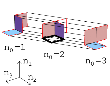
Figure 4: Sample closed vortex surface configuration. At each lattice time $n_{0}$, shaded plaquettes are part of the vortex surface. These plaquettes are furthermore connected to plaquettes running in time direction; their location can be inferred most easily by keeping in mind that each link of the configuration is connected to exactly two plaquettes (i.e. the surface is closed and contains no intersection lines). Note that the two non-shaded plaquettes at $n_{0}=2$ are not part of the vortex; only the sets of links bounding them are. These are slices at $n_{0}=2$ of surface segments running in time direction from $n_{0}=1$ through to $n_{0}=3$. Sliced at $n_{0}=2$, these surface segments show up as lines. The surface is non-orientable; the thick line at $n_{0}=2$ indicates a minimal non-contractible (monopole) loop on the surface at which the orientation is inverted. Note also that the topological charge $Q=1/2$ of the configuration is carried purely by surface writhings; there are no surface self-intersection points. The author gratefully acknowledges R. Bertle and M. Faber for providing the MATHEMATICA routine with which the image was generated.

Note furthermore that even the fact that a twisted torus does not directly permit a definition of fundamental quark fields should be seen more as a practical disadvantage than a fundamental one. By piecing copies of a twisted torus together such as to make up a larger torus with appropriate integer multiple extensions in the four space-time directions, one arrives at a description in terms of gauge fields with periodic boundary conditions on the larger torus. On this torus, quark fields can then be straightforwardly defined [28],[30]. The price one pays consists in having to work on a larger space-time manifold; of course, from the practical point of view of numerical Monte-Carlo calculations, this can be a decisive disadvantage.

5 Quenched Dirac spectrum of the random vortex surface model

In the following, results for the quenched ensemble average of the Dirac spectrum in the framework of the random vortex model of infrared Yang-Mills theory will be presented. The dynamics determining this model ensemble and its physical interpretation are discussed at length in [1]. The model describes closed vortex world-surfaces composed of elementary squares (plaquettes) on a hypercubic lattice. An ensemble of such world-surfaces is generated using Monte Carlo methods, where, in order to keep the surfaces closed, an elementary update of a vortex world-surface configuration always affects all six plaquettes making up the surface of a three-dimensional cube in the four-dimensional lattice; any of those six plaquettes which were not part of a vortex surface before the update become part of a vortex surface after the update, and vice versa. As mentioned in section 3.4, keeping track of the updated three-cubes directly allows the construction of the three-volume $\Sigma$ which is needed as input for the definition of a corresponding vortex gauge field, cf. section 3.1. The acceptance criterion, i.e. the Boltzmann factor $\exp(-S)$, for any given update depends on the curvature of the vortex surfaces. An additive action increment $c=0.24$ is contributed to $S$ by each pair of vortex plaquettes on the lattice sharing a link, but not lying in the same plane; the value of $c$ was chosen such as to quantitatively reproduce the confinement properties of $SU(2)$ Yang-Mills theory [1]. This vortex ensemble simultaneously yields a result for the topological susceptibility which quantitatively agrees with full $SU(2)$ Yang-Mills lattice calculations [2].

Given a particular vortex configuration, via the associated three-volume $\Sigma$, the Dirac matrix (in practice, a $2\times 2$ Dirac block of its square, cf. eq. (26)) can be constructed as described in sections 3 and 4.1. The 30 lowest-lying eigenvalues of this matrix were obtained using the ARPACK package [31], and (their positive square roots) binned according to their magnitude, yielding the density of eigenvalues (per unit space-time volume) $\rho(\lambda)$ of the Dirac operator. The behavior of this distribution near $\lambda=0$ is related to the chiral condensate $\langle\bar{q}q\rangle$ via the Casher-Banks formula [32],[33]

$$\langle\bar{q}q\rangle=-\lim_{V\rightarrow\infty}2m\int_{0}^{\infty}d\lambda\,\frac{\rho(\lambda)}{m^{2}+\lambda^{2}}\stackrel{{\scriptstyle m\rightarrow 0}}{{\longrightarrow}}-\pi\rho(0)$$ (31)

where $m$ denotes the quark mass and $V$ the space-time volume. A range of results obtained in this way is displayed in Figs. 5 and 6, with emphasis on the variation with volume. The two main features of these eigenvalue distributions are a bulk behavior which extrapolates to a finite non-zero value at $\lambda=0$, and an additional enhancement for very small eigenvalues which presumably signals the onset of divergent behavior at $\lambda=0$. In view of (31), such a divergence implies a diverging chiral condensate in the chiral limit $m\rightarrow 0$; at finite quark mass $m$, the enhancement near $\lambda=0$ generates an increase in the chiral condensate compared with the value one would extract from the bulk of the spectrum. On the other hand, in (31) the infinite volume limit is to be taken before the chiral limit, and Figs. 5 and 6 suggest that the enhancement of the spectra near $\lambda=0$ weakens as the space-time volume is increased. However, the limited statistics of the measurements precludes a solid extrapolation of the aforementioned enhancement to infinite volume; it is unclear whether it completely disappears as $V\rightarrow\infty$ or whether it approaches a nontrivial limit.

Divergences in the quenched chiral condensate reminiscent of the behavior observed here have been noted in a variety of contexts, and both of the aforementioned alternatives concerning the $V\rightarrow\infty$ limit have been discussed. An ensemble of vortex configurations extracted from the full $SU(2)$ lattice Yang-Mills ensemble using an appropriate gauge fixing and projection procedure yields a divergent chiral condensate in the chiral limit [16]. This phenomenon is also observed in quenched lattice calculations using domain wall fermions [18]. The main effect in this case is due to exact Dirac zero modes resulting from a nontrivial topological charge of the gauge configurations; this effect vanishes for $V\rightarrow\infty$ as has been argued at the end of section 4.1. On the other hand, this effect may also hide more subtle divergences which persist in the infinite volume limit. Such more persistent divergences have been argued to appear both in quenched chiral perturbation theory [34] and in instanton models [35]. In the latter models, the strength of the divergence strongly decreases as one leaves the dilute instanton gas limit and allows the associated quark zero modes to interact strongly. Note that, in contrast to the instanton picture, the present vortex picture does not possess an obvious dilute limit with weakly interacting quark quasi-zero modes. In view of this, the observation of a persistent divergence in the Dirac

Figure 5: Dependence of Dirac spectral density $\rho$ on the extension of space-time. Left: Gauge field constructed using random monopoles and random $\Sigma$; data symbolized by $\times$ corresponds to a $3^{4}$ lattice, crosses correspond to a $4^{4}$ lattice, and circles to a $5^{4}$ lattice. The reader is reminded that the lattice spacing is $0.39\,$fm. Right: Gauge field constructed using minimal monopoles and random $\Sigma$; data symbolized by $\times$ corresponds to a $3^{3}\times 2$ lattice, crosses correspond to a $4^{3}\times 2$ lattice, and circles to a $6^{3}\times 2$ lattice. Note that an extension of the lattice in Euclidean time direction of two spacings is equivalent to a temperature of $T=0.83\,T_{c}$.

spectrum as $V\rightarrow\infty$ in the instanton model does not straightforwardly imply the same qualitative effect in the vortex picture. More detailed information on this question may result from a consideration of the space-time structure of low-lying quark modes in the vortex model; such an investigation lies beyond the scope of the present work. Note also that, in unquenched calculations, the spectral density near zero eigenvalue will be dynamically suppressed due to the weighting with the determinant of the Dirac operator. Nevertheless, the aforementioned instanton model calculations still yield divergent behavior at $\lambda=0$, which however disappears as $m\rightarrow 0$ such as to yield a finite chiral condensate in the chiral limit.

Figure 6: Dependence of Dirac spectral density $\rho$ on the extension of space-time. The gauge field is constructed using minimal monopoles and smooth $\Sigma$. Data symbolized by $\times$ corresponds to a $3^{3}\times 2$ lattice, crosses correspond to a $4^{3}\times 2$ lattice, circles to a $5^{3}\times 2$ lattice, open boxes to a $6^{3}\times 2$ lattice, and filled boxes to a $7^{3}\times 2$ lattice.

If the Dirac spectrum retains divergent behavior at $\lambda=0$ even in the infinite volume limit, then the issue of the phenomenological relevance of this behavior becomes a subtle quantitative question. In view of (31), for sufficiently large quark masses the extra contribution to the chiral condensate resulting from the divergence at $\lambda=0$ becomes negligible and the condensate is dominated by the bulk spectral density. The question then remains whether realistic quark masses are large or small in this sense. While this caveat must be kept in mind, further below, numerical values for the chiral condensate will be quoted which correspond to the $\lambda=0$ extrapolation of the bulk of the spectral density, disregarding the enhancement of the spectrum very near $\lambda=0$.

Turning now to the properties of the bulk of the spectrum in more detail, Fig. 5 displays results for the “random $\Sigma$” construction of the gauge field with either minimal or random monopoles, respectively. In these cases, the bulk value evidently has already converged well to the large volume limit at a spatial extension of the universe corresponding to 4 lattice spacings, i.e. $4a=1.56\,$fm. In Fig. 6, exhibiting results for the “smooth $\Sigma$” construction with minimal monopoles, the convergence is not quite as fast; there is still a discrepancy of the order of $10\,$% between the universe with spatial extension $1.56\,$fm and the universe with spatial extension $1.95\,$fm, the results in the latter case being indistinguishable from those on larger lattices. The finite size effects were also considered in a number of other cases: Random $\Sigma$ with random monopoles on $n^{3}\times 1$ lattices, random $\Sigma$ with minimal monopoles on $n^{4}$ lattices and on $n^{3}\times 1$ lattices, and smooth $\Sigma$ with minimal monopoles on $n^{4}$ lattices. All these cases displayed a convergence to the large volume limit comparable to or better than the ones exhibited here explicitly. Also in the smooth $\Sigma$ case with random monopoles, the bulk of the spectrum on a $3^{4}$ lattice turns out to be indistinguishable from the one on a $4^{4}$ lattice.

In the following, Dirac spectra will be shown for different choices of the gauge field construction and different temperatures at a spatial extension of the lattice of $4a=1.56\,$fm. While one should be aware that this extension in some cases still allows for finite size effects of the order of $10\,$%, it does not suffer from the aforementioned subtlety (cf. footnote) arising for lattices with odd numbers of lattice sites in at least one of the space-time directions, and it also allows for superior statistics compared with extensions corresponding to the next even multiple of the lattice spacing, $6a=2.34\,$fm. The results are depicted in Figs. 7-9, and also summarized in Table 1.

Figure 7: Dependence of Dirac spectral density $\rho$ on temperature $T$, at a spatial extension of the lattice of $4a=1.56\,$fm. Left: Gauge field constructed using random monopoles and random $\Sigma$; data symbolized by $\times$ corresponds to $T=0$, circles correspond to $T=0.83\,T_{c}$, and crosses to $T=1.67\,T_{c}$. Right: Gauge field constructed using minimal monopoles and random $\Sigma$; data symbolized by $\times$ corresponds to $T=0$, circles correspond to $T=0.83\,T_{c}$, and crosses to $T=1.67\,T_{c}$.

Figure 8: Dependence of Dirac spectral density $\rho$ on temperature $T$, at a spatial extension of the lattice of $4a=1.56\,$fm. Left: Gauge field constructed using random monopoles and smooth $\Sigma$; data symbolized by $\times$ corresponds to $T=0$, circles correspond to $T=0.83\,T_{c}$, and crosses to $T=1.67\,T_{c}$. Right: Gauge field constructed using minimal monopoles and smooth $\Sigma$; data symbolized by $\times$ corresponds to $T=0$, circles correspond to $T=0.83\,T_{c}$, and crosses to $T=1.67\,T_{c}$.

Figure 9: Detailed plot of the (third root of the) Dirac spectral density $\rho$ obtained at a temperature of $T=1.67\,T_{c}$ for a spatial extension of the lattice of $4a=1.56\,$fm using the minimal monopole, smooth $\Sigma$ construction of the gauge field. The chiral condensate does not vanish in the deconfined phase, but is sharply reduced.

$$\begin{array}[]{|c||c|c|c|c|}\hline\cr&\lx@intercol\hfil-\langle\bar{q}q\rangle/\mbox{GeV}^{3}\hfil\lx@intercol\vrule\lx@intercol\\ \cline{2-5}\cr T/T_{c}&\mbox{minim. monop.}&\mbox{minim. monop.}&\mbox{random monop.}&\mbox{random monop.}\\ &\mbox{smooth }\Sigma&\mbox{random }\Sigma&\mbox{smooth }\Sigma&\mbox{random }\Sigma\\ \hline\cr\hline\cr 0&0.129&0.108&0.175&0.100\\ \hline\cr 0.83&0.094&0.100&0.157&0.097\\ \hline\cr 1.1&0.059&\mbox{---}&\mbox{---}&\mbox{---}\\ \hline\cr 1.4&0.0033&\mbox{---}&\mbox{---}&\mbox{---}\\ \hline\cr 1.67&0.0015&0.078&0.103&0.203\\ \hline\cr\end{array}$$

Table 1: Chiral condensate as a function of temperature for different gauge field constructions on a lattice of spatial extension 1.56 fm, obtained by extrapolating the bulk of the Dirac spectral density to zero eigenvalue. Since the inverses of the temperatures $T=1.1\,T_{c}$ and $T=1.4\,T_{c}$ are not integer multiples of the lattice spacing $a$ in the random surface model with curvature coefficient $c=0.24$, the associated values of the chiral condensate were obtained by the following interpolation procedure [1]. The inverse of $T=1.1\,T_{c}$ corresponds to one lattice spacing for $c=0.14$ and to two lattice spacings for $c=0.32$; interpolating $\langle\bar{q}q\rangle\,a^{3}$ as a function of $c$ defines the chiral condensate also at $c=0.24$ for $T=1.1\,T_{c}$. The same procedure was also applied to $T=1.4\,T_{c}$, the inverse of which corresponds to one lattice spacing for $c=0.2$ and to two lattice spacings for $c=0.407$.

Evidently, in the confined phase, all models yield a bulk spectral density which extrapolates to a nonzero value at $\lambda=0$, thus signaling the spontaneous breaking of chiral symmetry. Quantitatively, the zero-temperature quenched chiral condensate obtained for the different gauge field constructions varies between $-0.1\,\mbox{GeV}^{3}$ and $-0.175\,\mbox{GeV}^{3}$. For comparison, the value obtained in lattice Yang-Mills calculations [20] corresponds to $-0.09\,\mbox{GeV}^{3}$ (with the zero-temperature string tension fixed to the same value as in the present model). In particular, both of the random $\Sigma$ models come very close to the lattice Yang-Mills result. However, it should be kept in mind that the actual value of $\langle\bar{q}q\rangle$ does not have direct phenomenological meaning, since it is not a renormalization group invariant quantity. Only after multiplying with the quark mass, one obtains a physically meaningful quantity which enters e.g. current algebra relations. In this sense, a measurement of $\langle\bar{q}q\rangle$ can be viewed as representing no more than an accessory to defining the current quark masses within the model. However, the fact that the vortex model yields values for the chiral condensate which are not separated from lattice values by unnaturally large factors gives rise to the expectation that this model succeeds in capturing the relevant physics leading to spontaneous chiral symmetry breaking in the confined phase of the strong interaction. More stringent quantitative tests of low-energy quark physics within the vortex model demand the calculation of additional observables; this is deferred to future work.

Turning now to the behavior of the chiral condensate as one crosses the finite-temperature deconfinement transition, the different models evidently display much larger, qualitative, differences. The random $\Sigma$, random monopole model yields a considerably enhanced chiral condensate in the deconfined phase; the other models show a reduction of the condensate above the critical temperature. However, this reduction is rather slight, except in the case of the smooth $\Sigma$, minimal monopole model. This latter case is the only one which qualitatively agrees with lattice calculations [18]: The quenched chiral condensate does not disappear in the deconfined regime, but it is sharply reduced as one crosses the phase transition, cf. in particular Fig. 9. In view of the discussion of section 2, the fact that the smoothest choice of gauge field construction yields the most realistic physics is not unexpected. This appears to be the model of choice. As discussed above, the fact that it yields a value for the quenched chiral condensate in the confining phase which is slightly enhanced compared with lattice calculations has no direct phenomenological relevance. Alternatively, one could envisage ultimately using a minimal monopole model which interpolates between the smooth and random $\Sigma$ cases such as to reproduce the lattice results even more closely.

6 Summary

Three fundamental nonperturbative phenomena characterize the low-energy regime of the strong interaction: Confinement, the $U_{A}(1)$ flavor anomaly, and the spontaneous breaking of chiral symmetry. While the ($SU(2)$ color) random vortex world-surface model was shown to quantitatively describe the first two of the aforementioned phenomena in [1],[2], the present work indicates that also the third phenomenon, i.e. the spontaneous breaking of chiral symmetry, finds a viable description within this model. Specifically, a gauge field construction for vortex world-surface configurations was found which, coupled to quarks, leads to a behavior of the quenched chiral condensate as a function of temperature in qualitative agreement with the behavior found in lattice Yang-Mills theory. Quantitatively, the quenched chiral condensate $\langle\bar{q}q\rangle$ differs from the lattice Yang-Mills result by a factor of the order of unity which presumably can be absorbed into the ultraviolet regularization scheme dependence of the chiral condensate, or, equivalently, into the definition of the current quark mass $m$. Only the product $m\langle\bar{q}q\rangle$ is a renormalization group invariant, physical quantity which can be tested e.g. using current algebra techniques. Stringent quantitative tests of low-energy quark physics via additional hadronic observables are deferred to future work.

The main thrust of the present investigation lay in developing the technical tools necessary for such work. In order to incorporate quark physics into the vortex model, the Dirac operator in a vortex background had to be constructed. This involves, as a prerequisite, casting vortex configurations explicitly in terms of gauge fields. Having appropriately specified such vortex gauge fields via a Wu-Yang construction, a matrix representation of the Dirac operator in a truncated (finite element) quark basis was obtained which determines infrared quark propagation in the combined vortex-quark system. The evaluation of the quenched chiral condensate highlighted above represents a first exploratory application of these techniques.

With the Dirac operator at hand, one can envisage also carrying out dynamical quark calculations within the vortex model, by reweighting the vortex ensemble with the Dirac operator determinant. This will substantially penalize Dirac eigenvalues of very small magnitude and thus presumably reduce the chiral condensate to the phenomenologically expected values around $(230\,\mbox{MeV})^{3}$. Moreover, to make contact with phenomenology, the random vortex surface model must still be extended to $SU(3)$ color; also in the three-color case, lattice Yang-Mills measurements [36] indicate that vortex degrees of freedom dominate the infrared, confining sector of the strong interaction.

References

- [1] M. Engelhardt and H. Reinhardt, Nucl. Phys. B585 (2000) 591.
- [2] M. Engelhardt, Nucl. Phys. B585 (2000) 614.
- [3] G. ’t Hooft, Nucl. Phys. B138 (1978) 1.
- [4] Y. Aharonov, A. Casher and S. Yankielowicz, Nucl. Phys. B146 (1978) 256.
- [5] J. M. Cornwall, Nucl. Phys. B157 (1979) 392.
-
[6]
G. Mack and V. B. Petkova, Ann. Phys. (NY) 123
(1979) 442;
G. Mack, Phys. Rev. Lett. 45 (1980) 1378. -
[7]
H. B. Nielsen and P. Olesen, Nucl. Phys. B160
(1979) 380;
J. Ambjørn and P. Olesen, Nucl. Phys. B170 [FS1] (1980) 60; ibid. 265. - [8] L. Del Debbio, M. Faber, J. Greensite and Š. Olejník, Phys. Rev. D 55 (1997) 2298.
- [9] L. Del Debbio, M. Faber, J. Giedt, J. Greensite and Š. Olejník, Phys. Rev. D 58 (1998) 094501.
- [10] T. G. Kovács and E. T. Tomboulis, Phys. Rev. Lett. 85 (2000) 704.
- [11] K. Langfeld, O. Tennert, M. Engelhardt and H. Reinhardt, Phys. Lett. B452 (1999) 301.
- [12] M. Engelhardt, K. Langfeld, H. Reinhardt and O. Tennert, Phys. Rev. D 61 (2000) 054504.
- [13] R. Bertle, M. Faber, J. Greensite and Š. Olejník, JHEP 9903 (1999) 019.
- [14] R. Bertle, M. Engelhardt and M. Faber, Phys. Rev. D 64 (2001) 074504.
- [15] P. de Forcrand and M. D’Elia, Phys. Rev. Lett. 82 (1999) 4582.
- [16] C. Alexandrou, M. D’Elia and P. de Forcrand, Nucl. Phys. Proc. Suppl. 83 (2000) 437.
- [17] C. Alexandrou, P. de Forcrand and M. D’Elia, Nucl. Phys. A663 (2000) 1031.
- [18] G. T. Fleming, P. Chen, N. H. Christ, A. L. Kaehler, C. I. Malureanu, R. D. Mawhinney, G. U. Siegert, C.-Z. Sui, P. M. Vranas and Y. Zhestkov, Nucl. Phys. Proc. Suppl. 73 (1999) 207.
- [19] T. G. Kovács and E. T. Tomboulis, Phys. Rev. D 65 (2002) 074501.
- [20] S. J. Hands and M. Teper, Nucl. Phys. B347 (1990) 819.
- [21] T. T. Wu and C. N. Yang, Phys. Rev. D 12 (1975) 3843; ibid. 3845.
- [22] M. Faber, J. Greensite and Š. Olejník, Phys. Rev. D 57 (1998) 2603.
- [23] M. Engelhardt and H. Reinhardt, Nucl. Phys. B567 (2000) 249.
- [24] J. M. Cornwall, Phys. Rev. D 61 (2000) 085012.
- [25] H. Reinhardt, hep-th/0112215.
- [26] R. Bertle, M. Engelhardt and M. Faber, Nucl. Phys. Proc. Suppl. 106 (2002) 661.
-
[27]
G. ’t Hooft, Nucl. Phys. B153 (1979) 141;
P. van Baal, Comm. Math. Phys. 85 (1982) 529. - [28] M. García Pérez, A. González-Arroyo, C. Pena and P. van Baal, Nucl. Phys. B564 (2000) 159.
- [29] M. García Pérez, A. González-Arroyo, A. Montero, C. Pena and P. van Baal, Nucl. Phys. Proc. Suppl. 83 (2000) 464.
- [30] A. González-Arroyo, Nucl. Phys. B548 (1999) 626.
-
[31]
http://www.caam.rice.edu/software/ARPACK/. - [32] T. Banks and A. Casher, Nucl. Phys. B169 (1980) 103.
- [33] H. Leutwyler and A. Smilga, Phys. Rev. D 46 (1992) 5607.
-
[34]
C. Bernard and M. Golterman, Nucl. Phys. Proc. Suppl.
26 (1992) 360;
S. Sharpe, Nucl. Phys. Proc. Suppl. 30 (1993) 213. - [35] U. Sharan and M. Teper, hep-ph/9910216.
- [36] M. Faber, J. Greensite and Š. Olejník, Phys. Lett. B474 (2000) 177.