QCD VACUUM AND CONFINEMENT

Abstract

This course consists of two lectures. In the first lecture I discuss why a non perturbative formulation of QCD is needed ,and I show that lattice formulation copes with this need, even if it mainly produces numerical results. In the second lecture I discuss how lattice can help to understand the deconfinement transition.Such understanding is also important to predict parameters that can help in the interpertation of heavy ions high energy experiments.

1 Introduction

Vacuum is by definition the ground state of a field system:it is stable against quantum fluctuations.

An exact knowledge of the ground state provides complete information on the system.This property goes under the name of reconstruction theorem,the exact statement being that from the field correlators

$$\langle 0|T(\varphi_{1}(x_{1})\ldots\varphi_{n}(x_{n})|0\rangle$$ (1)

the Hilbert space and the matrix elements of physical observables can be constructed.

Textbook quantization is perturbative .The Lagrangean is split in a free term ${\cal L}_{0}$ and a perturbation ${\cal L}_{I}$

$${\cal L}={\cal L}_{0}+{\cal L}_{I}$$ (2)

${\cal L}_{0}$ is exactly solvable ,and defines as vacuum the ground state of Fock space,i.e. empty space. ${\cal L}_{I}$ is a small perturbation producing scattering between fundamental particles, and small changes in the wave function of the ground state.

In QCD ${\cal L}_{0}$ describes free gluons and quarks and their interactions. For sure this is not a good starting point ,since quarks and gluons are confined.Fock vacuum is not the ground state,and therefore it is not stable against perturbations.

This is most probably the reason why the perturbative expansion is not convergent,not even as an asymptotic series,in spite of the fact that it seems to work at small distances1 .

The knowledge of the true vacuum is,in particular,relevant to the understanding of one of the most intriguing properties of QCD, namely confinement of color.

In spite of the well established evidence that quarks and gluons are the fundamental constituents of hadronic matter, they have never been observed in Nature as free particles.

All particles produced in particle reactions are color singlets.This property is known as confinement of color.

Since the pioneering papers of Gellmann in which quarks were introduced as fundamental constituents of hadrons ,quarks have been searched for in particle reactions and in Nature.None has been found,so that experiments establish upper limits,which can be found in Particle Data Group2 . The cross section $\sigma_{q}$ for the inclusive reaction

$$p+p\to q\,(\bar{q})+X$$ (3)

in which a $q,\,(\bar{q})$ is detected as a fractionally charged particle has an upper limit

$$\sigma_{q}<10^{-40}\,{\rm cm}^{2}$$ (4)

to be compared to the total cross section $\sigma_{T}$ at the same energy $\sigma_{T}\sim 10^{-25}\,{\rm cm}^{2}$. In the absence of confinement $\sigma_{q}/\sigma_{T}$ would be of the order of unity,and is instead $\sigma_{q}/\sigma_{T}\simeq 10^{-15}$.

Similarily the abundance $n_{q}$ of free quarks in Nature is measured by looking for particles of fractional charge $q=\pm 1/3,\pm 2/3$ in Millikan like experiments.

No quarks have been found,and the resulting upper limit is $n_{q}/n_{p}<10^{-27}$ corresponding to the analysis of $\sim 1g$ of matter.

In the absence of confinement the Standard Cosmological Model (SCM) predicts $n_{q}/n_{p}\sim 10^{-12}$3 . Again a factor $10^{-15}$ between upper limit and expectation.

Such a small factor cannot have a natural theoretical explanation ,except if the actual value of the above quantities is exactly zero.Confinement is an absolute property,and this can only be explained in terms of a symmetry property of the vacuum.The knowledge of the true vacuum is necessary to understand confinement .A quantization procedure that is not based on perturbation theory is needed.

2 Feynman path integral4 and lattice formulation of QCD5 .

A quantum system is defined by the canonical variables ,$q,p$ and the Hamiltonian $H$. Solving the system means to construct a Hilbert Space on which $q,p$ act as operators obeying the equations of motion and the canonical equal-time commutation relations.

$$[q_{i},p_{j}]=i\delta_{ij}$$ (5)

A ground state must exist.

Field theory is a special case. The fields $\varphi_{i}(\vec{x},t)$ play the role of the $q$’s ,their conjugate momenta $\Pi_{i}(\vec{x},t)=\partial{\cal L}/\partial(\partial_{0}\varphi_{i}(\vec{x},t))$ the role of the $p$’s. The system has infinitely many degrees of freedom.To simplify the notation we shall refer in what follows to a system with one $q$ and one $p$ ,since our arguments will apply to any number of degrees of freedom. Problems with divergencies ,arising from infinite number of degrees of freedom are technical in nature and do not affect the arguments below.The same is for problems in defining the conjugate momenta, which are a consequence of gauge invariance.

Since the $|q\rangle$’s are a complete set of states ,the knowledge of the amplitudes

$$A(q^{\prime},t^{\prime},q,t)=\langle q^{\prime}|e^{-iH(t^{\prime}-t)}|q\rangle$$ (6)

contains all physical information.

Let us divide the time interval $t^{\prime}-t$ into $n+1$ intervals of equal length $\delta$,

$$\delta=\frac{t^{\prime}-t}{n+1}$$

$\delta$ is a small quantity in the limit of large $n$. We can write

$$e^{-iH(t^{\prime}-t)}=e^{-iH\delta}e^{-iH\delta}\ldots e^{-iH\delta}$$ (7)

the product of $n+1$ factors.

Again for the sake of notational simplicity we shall assume that

$$H=\frac{p^{2}}{2m}+V(q)$$ (8)

The generic case with linear terms in $p$ ,or $q$-dependent coefficients of $p^{2}$, $p$ only present technical complications ,but do not alter the results which follow.

The amplitude eq (6) becomes, by inserting eq (7) and a number of projectors on a complete set $\int dq|q\rangle\langle q|=1$

$$A=\int dq_{1}\ldots dq_{n}\langle q^{\prime}|e^{-iH\delta}|q_{n}\rangle\langle q_{n}|e^{-iH\delta}|q_{n-1}\rangle\ldots\langle q_{1}|e^{-iH\delta}|q\rangle$$ (9)

On the other hand ,by use of the well known Baker-Haussdorf formula

$$e^{-iH\delta}\simeq e^{-i\frac{p^{2}}{2m}\delta}e^{-iV(q)\delta}\left[1+{\cal O}(\delta^{2})\right]$$ (10)

so that

$$\langle q_{i+1}|e^{-iH\delta}|q_{i}\rangle=e^{-iV(q_{i})\delta}\langle q_{i+1}|e^{-i\frac{p^{2}\delta}{2m}}|q_{i}\rangle\left[1+{\cal O}(\delta^{2})\right]$$

and since

$$\langle q_{i+1}|e^{-i\frac{p^{2}\delta}{2m}}|q_{i}\rangle=\int\frac{dp}{2\pi}\langle q_{i+1}|p\rangle\langle p|q_{i}\rangle e^{-i\frac{p^{2}\delta}{2m}}=\int\frac{dp}{2\pi}e^{ip(q_{i+1}-q_{i})-i\frac{p^{2}\delta}{2m}}=e^{i\frac{m}{2\delta}(q_{i+1}-q_{i})^{2}}$$

finally

$$\langle q_{i+1}|e^{-iH\delta}|q_{i}\rangle\simeq e^{i\left[\frac{m}{2}\frac{(q_{i+1}-q_{i})^{2}}{\delta^{2}}-V(q_{i})\right]\delta}=e^{i\delta\,{\cal L}[q_{i}]}$$ (11)

Inserting eq(11) into eq (9)

$$A=\lim_{n\to\infty}\int\left[\prod_{1}^{n}dq_{i}\right]e^{i\int_{t}^{t^{\prime}}{\cal L}dt}$$ (12)

In the limit $n\to\infty$, $\delta\to 0$ and eq(11) becomes exact. Eq(12) is usually written as

$$A=\int\left[{\cal D}q\right]e^{iS[q^{\prime},t^{\prime},q,t]}$$ (13)

The limit in eq(12) defines an integral over an infinite number of variables (a functional integral) if it exists.The amplitude eq(6) is an integral over all paths from $(q,t)$ to $(q^{\prime},t^{\prime})$ and is defined as a limit of a lattice in time ,as the points of the lattice fill densely the time interval $(t,t^{\prime})$.

Exponentials in eq(11) are analytic functions : the construction allows an analytic continuation of the amplitude to euclidean time $-t\to\tau=-it$ If $J(t)$ is an arbitrary function in the time interval $(t,t^{\prime})$ we define

$$S_{J}\equiv S(q,t,t^{\prime})+\int_{t}^{t^{\prime}}dtq(t)J(t)$$

$$A_{J}(q^{\prime},t^{\prime},q,t)=\int[{\cal D}q]\,\exp\left[iS_{J}(q^{\prime},t^{\prime},q,t)\right]$$ (14)

In the discretized version,

$$\int_{t}^{t^{\prime}}dtq(t)J(t)=\sum_{i=1}^{n}q(t_{i})J(t_{i})$$

We define the amplitude

$$A(t^{\prime},t_{1}\ldots t_{k},t)=\langle q^{\prime},t^{\prime}|T(q(t_{1})\ldots q(t_{k}))|q,t\rangle\qquad t\leq t_{i}\leq t^{\prime}$$ (15)

by the same construction which led to eq(13) as a limit of a discretized integral

$$A(t^{\prime},t_{1}\ldots t_{k},t)=\int[{\cal D}q]\,q(t_{1})\ldots q(t_{k})e^{-iS[t^{\prime},t]}$$

It follows from the definition of $A_{J}$, eq.(14), that

$$A(t^{\prime},t_{1}\ldots t_{k},t)=i^{n}\frac{\delta^{n}}{\delta J(t_{1})\ldots\delta J(t_{k})}\left.A_{J}(q^{\prime},t^{\prime},q,t)\right|_{J=0}$$ (16)

We shall now compute the amplitude for immaginary times $A_{J}(q^{\prime},-iT;q,iT)$, in the limit $T\to\infty$ . We shall assume that the external current $J$ is different from zero only in the time interval . $-T/2\leq t\leq T/2$. Then, calling $|E_{n}\rangle$ a complete set of states with definite energy,

$$A_{J}(q^{\prime},-iT;q,iT)=\sum_{E_{n},E_{n^{\prime}}}\langle q^{\prime}|e^{-HT/2}|E_{n}\rangle\langle E_{n}-i\frac{T}{2}|E_{n^{\prime}},i\frac{T}{2}\rangle_{J}\langle E_{n^{\prime}}|e^{-HT/2}|q\rangle$$ (17)

since by assumption from $-T$ to $-T/2$ and from $T/2$ to $T$ the evolution is governed by $H$. In the limit of large $T$

$$A_{J}(q^{\prime},-iT;q,iT)\mathop{\simeq}_{T\to\infty}e^{-E_{0}T}\psi_{0}(q^{\prime})\psi_{0}^{*}(q)\langle 0|\int[{\cal D}q]\,e^{-S[J]}|0\rangle$$ (18)

$|0\rangle$ is the ground state and $E_{0}$ its energy. Excited states are exponentially depressed in the sum eq(17).Modulo a multiplicative constant which will be shown to be unimportant,the amplitude of eq(16) is then equal to

$$Z[J]=\langle 0|\int[{\cal D}q]\,e^{-S[J]}|0\rangle$$ (19)

and,as in eq’s(15),(16)

$$\langle 0|T(q(t_{1})\ldots q(t_{k}))|0\rangle=\left.\frac{\delta^{n}Z[J]}{\delta J(t_{1})\ldots\delta J(t_{k})}\right|_{J=0}$$ (20)

$Z[J]$ is known as the functional generator of the field correlators (20).

Since the field correlators fully describe the theory,knowledge of $Z[J]$ means solution of the system.In particular the euclidean Feynman integral uniquely identifies the true ground state of the theory.

Feynman integral quantization is more fundamental than perturbative quantization.

For QCD the euclidean functional integral will be

$$Z[J]=\int[{\cal D}A_{\mu}][{\cal D}\psi][{\cal D}\bar{\psi}]e^{-S_{J}[A,\bar{\psi},\psi]}$$ (21)

where the role of $q$ is plaied by the gluon fields $A_{\mu}$ ,the quark field $\psi$ and its hermitian conjugate $\bar{\psi}$. The integral is defined by discretizing a finite volume $V$ of space time to a lattice of spacing $a$ and taking first the limit in which the lattice spacing $a\to 0$, so that the lattice densely fills the volume $V$ ,and finally sending $V\to\infty$.

In QCD both limits exist . By renormalization group arguments the lattice spacing $a$, at a given value of the coupling constant $g$, is related to the physical momentum scale $\Lambda_{L}$ as

$$a\mathop{\simeq}_{g^{2}\to 0}\frac{1}{\Lambda_{L}}\exp(-\frac{b}{g^{2}})$$ (22)

where $b$ is minus the inverse of the first coefficient of the beta function of the theory and is positive ,because of asymptotic freedom. Eq.(22) will be valid at sufficiently small values of $g^{2}$.

At sufficiently small $g^{2}$ $a$ is small in physical units and the granularity of the lattice becomes irrelevant.

Moreover a mass gap exists in the theory (a non zero minimum mass) ,which determines a finite correlation length $\xi$. If the lattice is sufficiently large with respect to $\xi$ the infinite volume limit is reached. Lattice will be a good approximant to the continuum if

$$a\ll\xi\ll La$$

$L$ being the linear size of the lattice. Lattice calculations are in that case an element of the sequence eq(12) near to the limit.Lattice will also uniquely identify the ground state.

The symmetry of the ground state ,which is at the basis of the confinement mechanism can safely be studied on the lattice.

3 Feynman integral and perturbation theory.

The only known computable functional integral is the gaussian integral,with a lagrangean quadratic in the fields,which corresponds to free fields.

The action can be written as

$$S_{0}=\frac{1}{2}\int dxdy\varphi_{i}(x){\cal D}^{-1}_{ij}(x-y)\varphi_{j}(y)$$ (23)

The resulting equations of motion are $\delta S/\delta\varphi(x)=0$ or $\int{\cal D}^{-1}_{ij}(x-y)\varphi_{j}(y)=0$ . The matrix ${\cal D}^{-1}_{ij}(x-y)$ is the inverse of the propagator. For the scalar field

$${\cal D}^{-1}_{ij}(x-y)=(\partial^{2}+m^{2})\delta_{ij}\delta(x-y)$$

The discretized version for $S_{0}$ is

$$S^{0}_{L}=\frac{1}{2}a^{4}\sum_{ab}\varphi_{a}{\cal D}^{-1}_{ab}\varphi_{b}$$

${\cal D}^{-1}_{ab}$ is a symmetric matrix which can be diagonalized by an orthogonal transformation

$$O_{T}{\cal D}^{-1}O={\cal D}^{-1}_{diag}$$ (24)

The jacobian of the transformation is equal to 1 so that

$$Z=\int\prod d\varphi_{i}e^{-\frac{1}{2}a^{4}\sum\varphi_{i}^{2}({\cal D}^{-1}_{diag})_{ii}}=c(\det{\cal D})^{1/2}$$ (25)

The correlation functions are given by

$$\langle 0|T(\varphi_{i_{1}}(x_{1})\ldots\varphi_{i_{n}}(x_{n})|0\rangle=\frac{1}{Z}\int\prod d\varphi_{i}\varphi_{i_{1}}(x_{1})\ldots\varphi_{i_{n}}(x_{n})e^{-S_{0}}$$ (26)

The integral is easy to compute,again by diagonalizing ${\cal D}^{-1}_{ij}$ ,giving

$$c(\det{\cal D})^{1/2}\sum_{perm}\prod{\cal D}_{i_{a}i_{b}}$$

The sum runs over all possible choices of the pairs $i_{a},i_{b}$.

The only non zero correlators are the two point functions. The Hilbert space is Fock space. The generic correlator is the product of two point functions.

In the perturbative approach to quantization the action $S$ is split in a quadratic part $S_{0}$ and terms containing higher powers of the fields

$$S=S_{0}+S_{I}$$

The functional integral is then computed by expanding the weight in powers of $S_{I}$

$$Z=\int{\cal D}\varphi e^{-S_{0}-S_{I}}=\int{\cal D}\varphi e^{-S_{0}}\sum_{n}\frac{(-1)^{n}}{n!}S_{I}^{n}$$ (27)

$S_{I}$ is a polynomial in the fields. The generic correlation function is then given by

$$\langle 0|T(\varphi_{i_{1}}(x_{1})\ldots\varphi_{i_{n}}(x_{n})|0\rangle=\frac{1}{Z}\int\prod d\varphi_{i}e^{-S_{0}}\varphi_{i_{1}}(x_{1})\ldots\varphi_{i_{n}}(x_{n})\sum_{k}\frac{(-1)^{k}}{k!}S_{I}^{k}$$ (28)

and again is a gaussian integral which can be computed.

The result, a sum of products of propagators, is nothing but the well known Wick’s theorem,and each term corresponds to a Feynman diagram.

Eq(26) is the interchange of the order of two limits ,which is not always legitimate.

The perturbative expansion can be seen as the functional version of the saddle point method for evaluating ordinary integrals. Consider a one variable integral of the form

$$I=\int_{a}^{b}dx\,\exp(if(x))g(x)$$ (29)

If $f$ and $g$ are analytic in a domain of the complex plane including the real interval $(a,b)$ the path of integration can be deformed in that domain to include the points $\bar{x}$ where the phase $f(x)$ is stationary,i.e. $\frac{df}{dx}=0$. The neighborhood of these points will give the main contribution to the integral :far from it the phase factor is rapidly oscillating ,and the contribution to the integral negligible. The saddle point method consists in writing $I$ in the form

$$I=\int_{a,C}^{b}d\delta\,e^{if(\bar{x})+\frac{i}{2}f^{\prime\prime}(\bar{x})\delta^{2}}g(\bar{x}+\delta)\sum_{n}\frac{i^{n}R^{n}(\delta)}{n!})$$ (30)

where $R(\delta)=f-f(\bar{x})-\frac{1}{2}f^{\prime\prime}(\bar{x})\delta^{2}$ (the linear term drops at $\bar{x}$ ), and the factor multiplying the exponential is intended as a power series in $\delta$. The integral is then gaussian . If more saddle points $\bar{x}_{i}$ exist $I$ will be the sum of analogous expansions around $\bar{x}_{i}$ .

The method works in practice. No systematic control ,however,exists of the approximations involved.

For the Feynman integral the idea is the same, except that now there are infinitely many integration variables. The phase is the action $S$, the integration variables are the fields, and a saddle point

$$\frac{\delta S}{\delta\varphi(x)}=0$$ (31)

is nothing but a classical solution of the equations of motion.

The point $\bar{\varphi}=0$ is certainly a saddle point. Around it one can expand the action as

$$S[\varphi]=S[\bar{\varphi}]+\left.\frac{1}{2}\frac{\delta^{2}S}{\delta\varphi_{i}\delta\varphi_{j}}\right|_{\varphi=\bar{\varphi}}\delta_{i}\delta_{j}+S_{I}$$ (32)

For $\bar{\varphi}=0$ $S[\bar{\varphi}]=0$, $\frac{1}{2}\frac{\delta^{2}S}{\delta\varphi_{i}\delta\varphi_{j}}\delta_{i}\delta_{j}=S_{0}$ and the saddle point formula is identical to the perturbative expansion eq (27).

In general, if different saddle points exist,the expression for the partition function becomes

$$Z=\sum_{\bar{\varphi}_{i}}e^{-S[\bar{\varphi}_{i}]}\int[d\delta]e^{-\frac{1}{2}\frac{\delta^{2}S}{\delta\varphi_{i}\delta\varphi_{j}}\delta_{i}\delta_{j}}\sum_{n}\frac{(-1)^{n}}{n!}S_{I}^{n}$$

and all the classical solutions with finite action contribute.

Such solutions (if non trivial) are called instantons. In a non abelian gauge theory finiteness of the euclidean action means

$$\left|\int d^{4}xTr\left[G_{\mu\nu}(x)G_{\mu\nu}(x)\right]\right|<\infty$$

or that the field $G_{\mu\nu}$ decreases more rapidly than $1/r^{2}$ as $r\to\infty$. The fields $A_{\mu}$ at large distance are a pure gauge: $A_{\mu}=i\partial_{\mu}U\,U^{\dagger}$ with $U$ an element of the gauge group. A topological number exists which counts how many times in this mapping the group is covered when the point at infinity sweeps the sphere $S_{3}$ . The topological charge is

$$Q=\frac{1}{16\pi^{2}}\int d^{4}xTr\left[G_{\mu\nu}(x)G^{*}_{\mu\nu}(x)\right]$$

and is an integer. Explicit instanton solutions were found6 which are self dual or antiselfdual

$$G_{\mu\nu}=\pm G^{*}_{\mu\nu}$$

A non zero value of $Q$ implies then a non zero value of $G^{2}=G_{\mu\nu}G_{\mu\nu}$, or that $\langle 0|G^{2}|0\rangle\neq 0$, a phenomenon which is known as gluon condensation. $\langle G^{2}(x)\rangle$, which must be $x$ independent by translation invariance, is known as gluon condensate. A non zero value of $\langle G^{2}\rangle$ is a highly non-perturbative result . Indeed renormalization group dictates for $\langle G^{2}\rangle$ the form of an operator of dimension 4,

$$\langle G^{2}\rangle\simeq e^{-4/b_{0}g^{2}}$$ (33)

where $b_{0}>0$ is proportional to the first non zero coefficient of the beta function. An expression like eq(33) is non analytic at $g^{2}=0$, and therefore non expandable in a power series of $g^{2}$ . A complete classification of the instantonic solutions does not exist.Models have been developed based on quasi-solutions,consisting of ensembles of single instantons.If their average distance is large compared to their size the ensemble is called an instanton gas7 , if the overlapping is important the ensemble is called an instanton liquid8 . Attempts to improve perturbative expansion by adding to the perturbative saddle point the saddle points corresponding to instantons have been done during the years,starting from the pioneering approach of ref[7]. Although useful to describe chiral properties, instantons fail in accounting for confinement of color.

Instantons were at the basis of the SVZ9 sum rules of QCD: that approach, which will be described in next section, is based on the existence of condensates, the original idea being that instantons provide a slowly varying background field for quantum fluctuations.

4 Condensates.

The time ordered product of two currents $j_{\mu}(x),j_{\nu}(0)$, e.g. electromagnetic currents,can be written at short distances as a sum of local operators times c-number coefficients10 .

$$T(j_{\mu}(x)j_{\nu}(0))\simeq C^{0}_{\mu\nu}(x)I+C^{4}_{\mu\nu}(x)G^{a}_{\mu\nu}G^{a}_{\mu\nu}+C^{\psi}_{\mu\nu}(x)m\bar{\psi}\psi+\ldots$$ (34)

The operators in eq(34) are ordered by increasing order of dimension in mass. The expansion is rigorously valid in perturbation theory, but is assumed to hold also when perturbation theory is not expected to work. Take the vev of eq.(34) and Fourier transform. The left side gives

$$\Pi_{\mu\nu}(q)\equiv\int e^{iqx}\langle 0|T(j_{\mu}(x)j_{\nu}(0))|0\rangle d^{4}x=(q_{\mu}q_{\nu}-q^{2}g_{\mu\nu})\Pi(q^{2})$$ (35)

the tensor structure being dictated by gauge invariance.

The spectral representation reads

$$\Pi(q^{2})=\Pi(0)-q^{2}\int_{4m_{\pi}^{2}}^{\infty}\frac{ds}{s}\frac{R(s)}{s-q^{2}+i\varepsilon}$$ (36)

with

$$R(s)=\frac{\sigma_{e^{+}e^{-}\to hadrons}}{\sigma_{e^{+}e^{-}\to\mu^{+}\mu^{-}}}$$

The right side of eq.(34) gives

$$(q_{\mu}q_{\nu}-q^{2}g_{\mu\nu})\left\{C_{0}(q^{2})+C_{g}(q^{2})G_{2}+C_{\psi}(q^{2})\langle m\bar{\psi}\psi\rangle+\ldots\right\}$$ (37)

The term $C_{0}(q)$ corresponds to the usual perturbative expansion and is constant modulo log’s. The other terms, known as ”higher twists”, are non perturbative in nature.

The approximate equality

$$-q^{2}\int_{4m_{\pi}^{2}}^{\infty}\frac{ds}{s}\frac{R(s)}{s-q^{2}+i\varepsilon}\simeq\left\{C_{0}(q^{2})+C_{g}(q^{2})G_{2}+C_{\psi}(q^{2})\langle m\bar{\psi}\psi\rangle+\ldots\right\}$$ (38)

can be exploited by appropriate weighting which emphasises the region where the equality is a good approximation on the average:the procedure is known as sum rules9 .

The dispersion integral in eq (38) is evaluated by inserting for $R(s)$ the resonances at low s and a constant above some threshold. A nice phenomenology results,relating resonance parameters to the condensates,which can be determined consistently giving9

$$\begin{array}[]{ll}G_{2}&=0.012\,{\rm GeV}^{4}\\ \langle\bar{\psi}\psi\rangle&=-0.13\,{\rm GeV}^{3}\end{array}$$

A more recent determination for $G_{2}$ is11

$$G_{2}=(0.024\pm 0.011)\,{\rm GeV}^{4}$$

5 Lattice determination of the condensates.

Consider the gauge invariant correlator

$${\cal D}_{\mu\nu,\rho\sigma}^{C}(x)=\langle 0|Tr\left\{G_{\mu\nu}(x)S_{C}(x,0)G_{\rho\sigma}(0)S_{C}^{\dagger}(x,0)\right\}|0\rangle$$ (39)

where $G_{\mu\nu}=\sum_{a}\frac{\lambda^{a}}{2}G^{a}_{\mu\nu}$, $A_{\mu}=\sum_{a}\frac{\lambda^{a}}{2}A^{a}_{\mu}$ and $\lambda^{a}$ are the generators of the gauge group in the fundamental representation.

$$S_{C}(x,0)=P\left\{\exp(i\int_{0,C}^{x}A_{\mu}(x)dx^{\mu})\right\}$$

is the parallel transport from 0 to $x$ along the path $C$. Under a gauge transformation $U(y)$, $S_{C}(x,0)\to U(x)S_{C}U^{\dagger}(0)$, which makes ${\cal D}_{\mu\nu,\rho\sigma}^{C}$ gauge invariant. In what follows we will chose for $C$ the straight line connecting 0 and $x$. ${\cal D}_{\mu\nu,\rho\sigma}^{C}$ can be considered as the split point regulator a la Schwinger of the gluon condensate $G_{2}$. The Wilson operator product expansion gives indeed

$${\cal D}_{\mu\nu,\rho\sigma}^{C}(x)\mathop{\simeq}_{x\to 0}\frac{c_{1}}{x^{4}}\langle I\rangle+c_{4}G_{2}$$ (40)

whence $G_{2}$ can be extracted. Poincare’ invariance implies12

$${\cal D}_{\mu\nu,\rho\sigma}(x) = (g_{\mu\rho}g_{\nu\sigma}-g_{\mu\sigma}g_{\nu\rho})[D(x)+D_{1}(x)]+$$

$$+(x_{\mu}x_{\rho}g_{\nu\sigma}-x_{\nu}x_{\rho}g_{\mu\sigma}-x_{\mu}x_{\sigma}g_{\nu\rho}+x_{\nu}x_{\sigma}g_{\mu\rho})\frac{\partial D_{1}}{\partial x^{2}}$$

or,choosing the $x^{0}$ axis along $x^{\mu}$ one can define13

$${\cal D}_{||} = \frac{1}{3}\sum_{i=1}^{3}{\cal D}_{0i,0i}=D+D_{1}+x^{2}\frac{\partial D_{1}}{\partial x^{2}}$$

$${\cal D}_{\perp} = \frac{1}{3}\sum_{i,j}{\cal D}_{ij,ij}=D+D_{1}$$

On the lattice,which is a formulation in terms of parallel transports, the correlators are easy to implement: the field strength is the open plaquette, the parallel transport the product of elementary links. The correlator is measured as the average on the ensemble of the configurations produced by MonteCarlo simulations of the operator:

${\cal D}^{L}_{\mu\nu\rho\sigma}=\left\langle\hbox{ \includegraphics[width=173.44534pt]{dis1.eps} }\right.$

$-\frac{1}{N_{c}}\left.\hbox{ \includegraphics[width=216.81pt]{dis2.eps}}\right\rangle$

${P}_{\mu\nu}$

${P}_{\rho\sigma}$                              ${P}_{\mu\nu}$             ${P}_{\rho\sigma}$

The figure represents the product of elementary links. The correlators $D$ and $D_{1}$ are plotted versus the distance in fm in fig. 1.

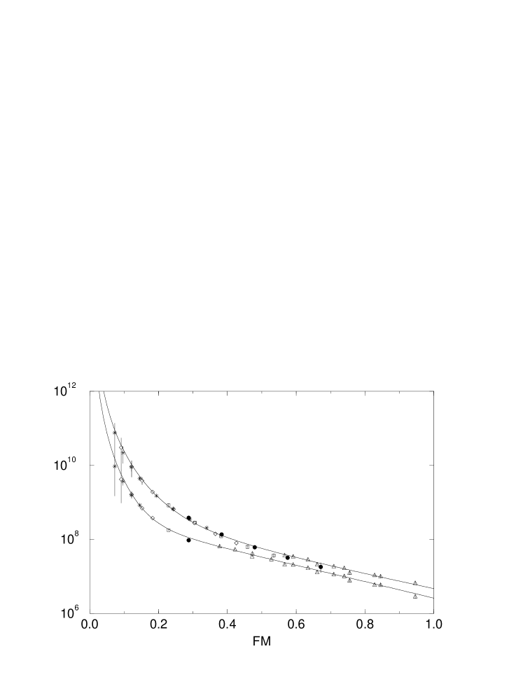
Figure 1: $D$ (upper curve) and $D_{1}$ vs distance in fm, as determined on lattice13 ; 14 .

The lines represent a best fit of the form

$$D = Ae^{-x/\lambda}+\frac{a}{|x|^{4}}$$ (42)

$$D_{1} = Be^{-x/\lambda}+\frac{b}{|x|^{4}}$$

which corresponds to the OPE eq.(40). One can extract $A$, $B$ and the correlation length $\lambda$. $G_{2}$ is proportional, with known coefficients to $A+B$. The result is

$$\begin{array}[]{lll}\hbox{ Quenched\cite[cite]{\@@bibref{Authors Phrase1YearPhrase2}{15}{\@@citephrase{(}}{\@@citephrase{)}}}}\hskip 7.22743ptSU(2)&G_{2}=(.33\pm.01)\,{\rm GeV}^{4}&\lambda=.16\pm.02\,{\rm fm}\\ \hbox{ Quenched\cite[cite]{\@@bibref{Authors Phrase1YearPhrase2}{13,14}{\@@citephrase{(}}{\@@citephrase{)}}}}\hskip 7.22743ptSU(3)&G_{2}=(.15\pm.03)\,{\rm GeV}^{4}&\lambda=.22\pm.02\,{\rm fm}\\ \hbox{Full QCD, extrapolated}&G_{2}=(.022\pm.005)\,{\rm GeV}^{4}&\lambda=.34\pm.03\,{\rm fm}\\ \hbox{to physical q masses\cite[cite]{\@@bibref{Authors Phrase1YearPhrase2}{16}{\@@citephrase{(}}{\@@citephrase{)}}}}&&\end{array}$$

The value of $G_{2}$ for full QCD agrees with recent phenomenological determinations11 . The correlation length is definitely too small in quenched theories, both SU(2) and SU(3) to consider the background field as slowly varying, it is slightly larger in full QCD.

By similar techniques the chiral condensate can be extracted from the correlator17

$${\cal D}_{\psi}(x)=m\langle\bar{\psi}(x)S_{C}(x,0)\psi(0)\rangle$$

which allows the OPE

$${\cal D}_{\psi}(x)\simeq\frac{C_{1}}{|x|^{2}}+C_{2}\langle m\bar{\psi}\psi\rangle$$

6 The stochastic vacuum.

In the Schwinger gauge $(x-z_{0})^{\mu}A_{\mu}(x)=0$, the gauge field $A_{\mu}$ can be expressed in terms of $G_{\mu\nu}$

$$A_{\mu}^{a}(x)=\int\alpha d\alpha(x-z_{0})G^{a}_{\mu\nu}(z_{0}+\alpha(x-z_{0}))$$ (43)

and any physical quantity can be expressed in terms of correlators of field strengths in the vacuum. A cluster expansion is made, and the assumption that higher correlators are products of two point correlators, higher clusters being negligible (stochastic vacuum model). The two point correlators determined on the lattice are used as an input, and several physical quantities can be computed: the heavy $q\bar{q}$ bound states or high energy cross sections. A successfull phenomenology results18 .

We have shown that non perturbative effects, like gluon condensate, are important in QCD and can be studied on the lattice. In the next lecture we shall investigate what symmetry of the vacuum is at the origin of color confinement.

7 Confinement of color.

A deconfinement transition is observed in lattice simulations of QCD.

The static thermodynamics of a field system at temperature T is described by the partition function

$$Z=tr\left\{e^{-H/T}\right\}$$

It is a known theorem that $Z$ is given by a Feynman euclidean integral, extending on the 3-dimensional physical space and on the time interval $(0,1/T)$, with periodic boundary conditions for bosons,antiperiodic for fermions.

On the lattice $Z$ is obtained by simulating the theory on a lattice $N_{S}^{3}\times N_{T}$ ,with $N_{S}\gg N_{T}$. In terms of the lattice spacing $a$ the temperature is then given by $T=1/N_{T}a$. The only free parameter in the simulation is the gauge coupling constant $g^{2}$ or better the parameter $\beta=2N_{c}/g^{2}$. In terms of $\beta$ the lattice spacing can be written as [see eq(22)]

$$a=\frac{1}{\Lambda}\exp(-\frac{\beta}{b})$$

or

$$T=\frac{1}{N_{T}a}=\frac{\Lambda}{N_{T}}\exp(\frac{\beta}{b})$$ (44)

Low temperature corresponds to small $\beta$ (strong coupling), high temperature to large $\beta$ (weak coupling).

This is the opposite to what happens in ordinary spin systems, where the temperature plays the role of coupling constant, and is due to asymptotic freedom. Confinement, for pure gauge theories, is related to the Polyakov line, which is the parallel transport along the time (temperature) axis from 0 to N, closed by periodic boundary conditions. The vev of the Polyakov line $\langle L\rangle$ can be interpreted as $\exp(-\mu_{q})$, $\mu_{q}$ being the chemical potential of an isolated quark. In the confined phase $\mu_{q}=\infty$, $\langle L\rangle=0$, while one can have $\langle L\rangle\neq 0$ in the deconfined phase. $\langle L\rangle$ can be called an order parameter for confinement, the symmetry being $Z_{N}$. What is usually determined on the lattice19 is the correlator of two Polyakov lines, which by cluster property behaves at large distances as

$$G(d)=\langle L(\vec{x})\bar{L}(\vec{y})\rangle\simeq A\exp(-\sigma daN_{T})+|\langle L\rangle|^{2}$$ (45)

with $d=|\vec{x}-\vec{y}|$.

The energy of two static quarks at distance $d$ is related to $G(d)$ by the equation

$$V(d)=-\frac{1}{aN_{T}}\log(G(d))$$ (46)

What is found on the lattice is that a temperature $T_{c}$ exists such that

$$\begin{array}[]{llll}T<T_{c}\hskip 10.84006pt&|\langle L\rangle|=0\hskip 10.84006pt&V(d)\mathop{\simeq}_{d\to\infty}\sigma d\hskip 10.84006pt&\hbox{(Confinement)}\\ T>T_{c}&|\langle L\rangle|\neq 0&V(d)\mathop{\simeq}_{d\to\infty}{\rm const.}&\hbox{(Deconfinement)}\end{array}$$

For quenched $SU(2)$ one finds $T_{c}/\sqrt{\sigma}\simeq 0.7$.

A finite size scaling analysis of $G$ at different spatial sizes $N_{S}$, allows to extract the critical index $\nu$ The result is $\nu\simeq 0.62$. The phase transition belongs to the same class of universality as the 3d ising model,as expected20 . For quenched $SU(3)$ the transition is found to be weak first order, $\nu=1/3$ and $T_{c}/\sqrt{\sigma}=0.65$ which means $T_{c}=270$ Mev if the conventional value $\sqrt{\sigma}=425$ MeV is assumed for the string tension.

In the presence of quarks $\langle L\rangle$ cannot be an order parameter, since the symmetry $Z_{N_{c}}$ is explicitely broken by the very presence of the quarks. At $m_{q}=0$, the chiral limit, an order parameter is the chiral condensate $\langle\bar{\psi}\psi\rangle$: however in reality the chiral symmetry is explicitely broken by quark masses. This variety of order parameters contrasts with the ideas of the limit $N_{c}\to\infty$.

The idea is that the number of colors $N_{c}$ can be considered as a parameter of the theory. In the limit $N_{c}\to\infty$ with $g^{2}N_{c}=\lambda$ fixed, a theory is defined , which differs little from the theory at finite $N_{c}$, say $N_{c}=3$.

In this spirit the mechanism of confinement should be fixed by the limiting theory ,and be essentially the same at all values of $N_{c}$ .

Quark loops being non leading in the expansion ,the mechanism of confinement should be the same in full QCD and in quenched theory.

The symmetry of the vacuum which is behind confinement, as explained in sect (1) should be $N_{c}$ independent. In this respect the existing situation for the order parameters looks rather confusing.

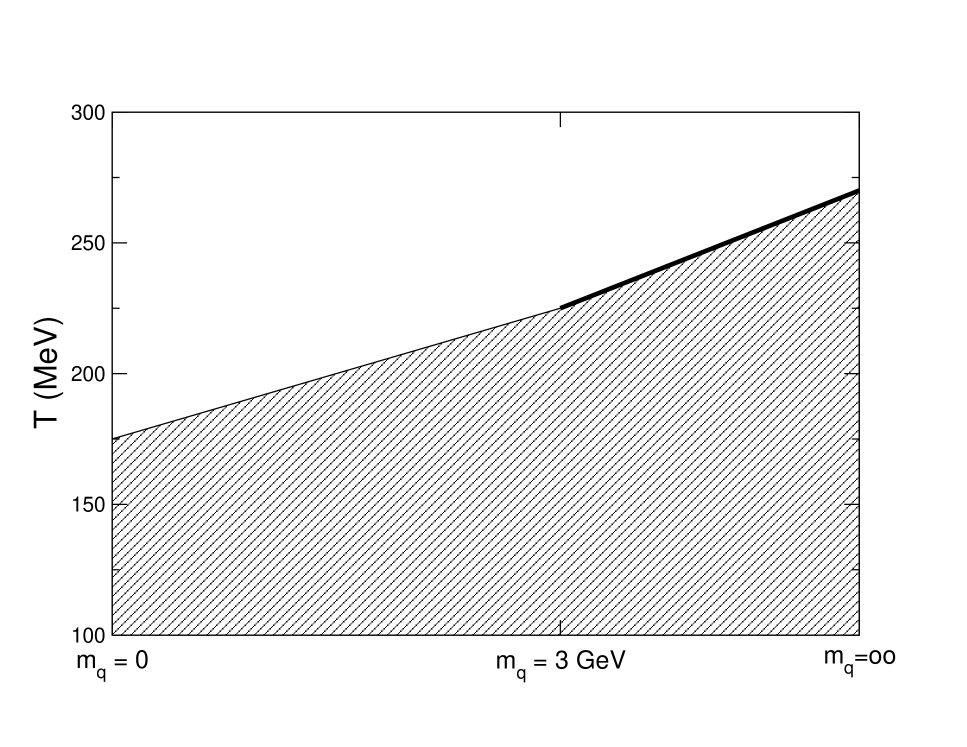
Figure 2: A schematic phase dyagram for 2 flavour QCD. Shaded area is confined, upper area deconfined.

Fig.2 shows schematically the phase dyagram for 2-flavor QCD as a function of the quark masses. The border between confined and deconfined phases is defined as the simultaneous maximum of various susceptibilities21 . ¿From $m_{q}=\infty$ to $m_{q}=3$ GeV the transition is first order, and the Polyakov line works as an order parameter as in quenched QCD. At $m_{q}=0$ there are arguments that the transition is second order22 . In the central region none of the susceptibilities which have been determined ($\bar{\psi}\psi$, susceptibility, derivative of the specific heat) goes large at the border between the two regions as the volume goes to infinity, and the conclusion is that maybe there is no transition, but only a crossover.

Still, if the deconfining transition is a change of symmetry,as argued in sect.1, there must exist an order(or disorder) parameter which distinguishes confined from deconfined, possibly the same as in quenched theory,in the line of $N_{c}\to\infty$ ideas.

8 Duality

The symmetry responsible for confinement has to be a symmetry of the (strong coupling) confining phase, which, in the langauge of statistical mechanics, is disordered. The natural question is: what can be the symmetry of a disordered phase? The answer is in a known concept in statistical mechanics, namely duality23 . $d$ dimensional systems admitting non local configurations with non trivial topology in $d-1$ dimensions, can have two complementary descriptions.

One description in terms of the ordinary local fields $\phi$,in which topological excitations $\mu$ are non local, and $\langle\phi\rangle$ are the order parameters; this description is convenient in the weak coupling regime $g\ll 1$ (ordered phase).

The other one ,dual description,in which the excitations $\mu$ become local fields ,their vev’s $\langle\mu\rangle$ are the order parameters: the coupling constant $g_{D}$ in this description is related to the original $g$ as $g_{D}\sim 1/g$. Duality maps the strong coupling regime of the direct description into the weak coupling regime of the dual.

A number of systems admitting dual descriptions are known in the literature.The prototype system is the 2d Ising model24 , in which the dual excitations are kinks, and the dual description is again a 2d ising model with $g_{D}\sim 1/g$; the N=2 SUSY QCD of ref25 , in which dual excitations are monopoles; the 3d XY model26 where the dual excitations are vortices,and the Heisenberg magnet in 3d, where the dual excitations are 2d Weiss domains27 . In QCD the dual excitations are not exactly known, but important information on their properties exists as we shall see below.

Two main candidates were originally proposed:

• monopoles28 ; 29 . Their condensation in the confining vacuum generates magnetic superconductivity,in the same way as the condensation of Cooper pairs generates ordinary superconductivity.

  The chromoelectric field between a $q\bar{q}$ pair is channeled into electric Abrikosov flux tubes, so that energy is proportional to the distance.

• $Z_{N}$ vortices30

In what follows we shall analyze the option a). As for vortices we refer to31 ; 32 and to references therein.

9 Basic superconductivity33 .

Before looking for dual (magnetic) superconductivity,we recall the basic concepts of ordinary superconductivity. The Landau-Ginzburg34 density of free energy (effective lagrangean) is determined by arguments of symmetry and of scale.

$${\cal L}=-\frac{1}{4}F_{\mu\nu}F_{\mu\nu}+\frac{1}{2}(D_{\mu}\phi)^{*}D_{\mu}\phi+\frac{m^{2}}{2}\phi^{*}\phi-\frac{\lambda}{4}(\phi^{*}\phi)^{2}+\hbox{irrelevant terms}$$ (47)

$\phi$ is a charged scalar field describing Cooper pairs , $D_{\mu}=\partial_{\mu}-iqA_{\mu}$ is the covariant derivative and the irrelevant terms are those of dimension higher than 4. $m^{2}=m^{2}(T)$ and $\lambda=\lambda(T)$ depend on the temperature.

For $T<T_{c}$ $m^{2}>0$ and the potential has a mexican hat shape as a function of $R(\phi)$ an of $Im(\phi)$.

For $T>T_{c}$ $m^{2}<0$ and the minimum of the potential is at $\phi=0$. If we parametrize $\phi=\rho e^{iq\theta}$, then $\tilde{A}_{\mu}=A_{\mu}-\partial_{\mu}\theta$ is a gauge invariant quantity: indeed under a gauge transformation $A_{\mu}\to A_{\mu}+\partial_{\mu}\Lambda$, $\theta\to\theta+\Lambda$. In terms of the new variables

$${\cal L}=-\frac{1}{4}F_{\mu\nu}F_{\mu\nu}+\frac{q^{2}\rho^{2}}{2}\tilde{A}_{\mu}\tilde{A}_{\mu}+\frac{1}{2}(\partial_{\mu}\rho)^{2}+\frac{m^{2}}{2}\rho^{2}-\frac{\lambda}{4}\rho^{4}$$ (48)

A static homogeneous solution is $\rho=\bar{\rho}$, a constant. The effective lagrangean for the photon is in that case

$${\cal L}=-\frac{1}{4}F_{\mu\nu}F_{\mu\nu}+q^{2}\bar{\rho}^{2}\tilde{A}_{\mu}\tilde{A}_{\mu}$$

The equation of motion is

$$\vec{\nabla}\wedge\vec{H}+q^{2}\rho^{2}\vec{\tilde{A}}=0$$ (49)

Taking the curl of both sides of eq(49)

$$\nabla^{2}\vec{H}-q^{2}\rho^{2}\vec{H}=0$$ (50)

The second term in eq (49) is a gauge invariant current,and is known as London current.

A non zero current with zero electric field means zero resistivity or superconductivity.

Eq(50) means that the magnetic field has a finite penetration depth in the superconductor , $1/q\rho$, and this is nothing but Meissner effect. If $m\gg q\bar{\rho}$ the superconductor is named Type II. In that case, when trying to introduce a magnetic field in the bulk, a penetration through separated Abrikosov flux tubes is energetically favoured.

Outside the tube $\tilde{A}=0$ and $\oint_{C}\vec{\tilde{A}}d\vec{x}=0$, $C$ being a path which encercles the flux tube. Since $\vec{\tilde{A}}=\vec{A}-\vec{\nabla}\phi$, this means

$$\int_{C}\vec{A}\,d\vec{x}=\int_{C}\vec{\nabla}\,d\vec{x}=\frac{2\pi n}{q}$$ (51)

The magnetic flux in the tube is quantized (Dirac quantization condition). A flux tube is to all effects a monopole antimonopole pair sitting at the ends with energy proportional to the length.

The order parameter of the system is $\Phi=q\bar{\rho}$, the vev of a charged field.

10 Monopoles in QCD.

Monopoles are always abelian35 : the magnetic monopole term in the multipole expansion of the field produced at large distances by any hadronic matter distribution ,obeys abelian field equations,and can always be reduced by a gauge transformation to the form $(0,0,a/r)$ in polar coordinates, with

$$a_{\varphi}=Q(1-\cos\theta)$$ (52)

and the Dirac string along the north pole. The $N_{c}\times N_{c}$ matrix $Q$ obeys the condition $e^{ig4\pi Q}=1$, implying that,in the representation in which $Q$ is diagonal, it has integer or half integer eigenvalues in units $1/g$. A monopole is identified by a constant diagonal matrix of the algebra with integer or half integer matrix elements: there exist $N_{c}-1$ independent monopole charges.

The same result follows from the procedure known as abelian projection28 . We shall illustrate it for the case of SU(2) gauge group: generalization to arbitrary $N_{c}$ is straightforward. Let be any field in the adjoint representation. Define $\hat{\phi}=\vec{\phi}(x)/|\vec{\phi}(x)|$, a direction in color space, and

$$F_{\mu\nu}=\hat{\phi}\cdot\vec{G}_{\mu\nu}-\frac{1}{g}\hat{\phi}\left(D_{\mu}\hat{\phi}\wedge D_{\nu}\hat{\phi}\right)$$ (53)

Both terms in the expression (53) are color singlets and gauge invariant.The combination is chosen in such a way that bilinear terms $A_{\mu}a_{\nu}$ and $A_{\mu}\partial_{\nu}\phi$ cancel. Indeed, by explicit computation

$$F_{\mu\nu}=\hat{\phi}(\partial_{\mu}\vec{A}_{\nu}-\partial_{\nu}\vec{A}_{\mu})-\frac{1}{g}\hat{\phi}(\partial_{\mu}\hat{\phi}\wedge\partial_{\nu}\hat{\phi})$$ (54)

A gauge transformation which brings $\hat{\phi}$ to a constant, e.g. to $(0,0,1)$ is called an abelian projection on $\vec{\phi}(x)$. In that gauge indeed

$$F_{\mu\nu}=\partial_{\mu}(\hat{\phi}\vec{A}_{\nu})-\partial_{\nu}(\hat{\phi}\vec{A}_{\mu})$$ (55)

is an abelian field. If, in the usual notation $F^{*}_{\mu\nu}=\varepsilon_{\mu\nu\rho\sigma}F_{\rho\sigma}$, a magnetic current can be defined as

$$j_{\nu}=\partial_{\mu}F^{*}_{\mu\nu}$$ (56)

This current is identically conserved, because of the antisymmetry of $F^{*}_{\mu\nu}$

$$\partial_{\nu}j_{\nu}=0$$ (57)

and identifies a $U(1)$ magnetic symmetry of the system.

In the usual continuum formulation $j_{\nu}$ is zero (Bianchi identities).

In a compact formulation, like lattice, $j_{\nu}$ can be non zero.

The U(1) magnetic symmetry can be either realized à la Wigner, and then the Hilbert space consists of superselected sectors with definite magnetic charge, or can be Higgs broken. In the first case the vev $\langle\mu\rangle=\langle 0|\mu|0\rangle$ of any operator $\mu$ carrying magnetic charge is strictly zero. In the second case there exists some $\mu$ such that $\langle\mu\rangle\neq 0$.

The effective action for $\langle\mu\rangle$ will then be of the form eq(47) and the system behaves as a dual superconductor. The operator $\mu$ is a disorder operator

$\langle\mu\rangle\neq 0$	in the disordered,confining phase
$\langle\mu\rangle=0$	in the ordered, deconfined phase

A magnetically charged operator $\mu$ can be constructed,which is magnetically charged in any given abelian projection36 ; 37 . The basic principle to construct $\mu$ is the well known formula for translations

$$e^{ipa}|x\rangle=|x+a\rangle$$ (58)

In field theory the field $\phi(y)$ is the analog of $x$. Its conjugate momentum $\Pi(y)$ the analog of $p$, and the operator

$$\mu(\vec{x},t)=\exp\left[i\int d^{3}\vec{y}\,\Pi(\vec{y},t)\tilde{\phi}(\vec{x}-\vec{y})\right]$$ (59)

gives

$$\mu(\vec{x},t)|\phi(\vec{y},t)\rangle=|\phi(\vec{y},t)+\tilde{\phi}(\vec{x}-\vec{y})\rangle$$ (60)

i.e. it adds the classical configuration $\tilde{\phi}(\vec{x}-\vec{y})$ to any field configuration.

For monopoles the field is $\vec{A}(\vec{x},t)$, the conjugate momentum $\partial_{0}\vec{A}(\vec{x},t)=\vec{E}(\vec{x},t)$, and the classical configuration to be added is the vector potential generated at the point $\vec{y}$ by a monopole sitting at the point $\vec{x}$, e.g.

$$\vec{b}(\vec{x}-\vec{y})=-\frac{m}{2e}\frac{\vec{n}\wedge\vec{r}}{r(r-\vec{n}\vec{r})}$$

where the Dirac string has been put along the $\vec{n}$ axis. The definition (60) has to be adapted to compact formulation .The details are published in ref37 . The result is of the form

$$\langle\mu(\vec{x},t)\rangle=\frac{\tilde{Z}(\beta,\vec{x},t)}{Z(\beta)}\qquad\beta=\frac{2N_{c}}{g^{2}}$$ (61)

where $Z(\beta)$ is the partition function

$$Z(\beta)=\int[{\cal D}A][{\cal D}\psi][{\cal D}\bar{\psi}]\exp(-\beta S_{E})$$

and

$$\tilde{Z}(\beta)=\int[{\cal D}A][{\cal D}\psi][{\cal D}\bar{\psi}]\exp(-\beta\tilde{S}_{E})$$

$\tilde{S}_{E}$ differs from $S_{E}$ by the introduction of a dislocation on the slice $x^{0}=t$. $\Delta S$ is proportional to the spatial volume, and therefore fluctuates as $N_{S}^{3/2}$, so that $\tilde{Z}$ fluctuates as $\exp(N_{S}^{3/2})$. It proves convenient to define instead

$$\rho(\beta)\equiv\frac{d}{d\beta}\log\langle\mu\rangle=\langle S\rangle_{S}-\langle S+\Delta S\rangle_{S+\Delta S}$$ (62)

which is easier to measure.In terms of $\rho$

$$\langle\mu\rangle=\exp\int_{0}^{\beta}\rho(\tau)d\tau$$ (63)

Fig.3 shows schematically the shape of $\langle\mu\rangle$ as a function of $\beta$, and that of $\rho$ .

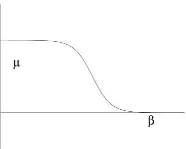
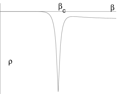
Figure 3: Typical dependence on $\beta$ of $\mu$ and $\rho$.

For $\beta<\beta_{c}$ (confinement) $\langle\mu\rangle\neq 0$, for $\beta>\beta_{c}\qquad\langle\mu\rangle=0$, at $\beta\sim\beta_{c}$

$$\langle\mu\rangle\sim(\beta-\beta_{c})^{\delta}\equiv(1-\frac{T}{T_{c}})^{\delta}$$

For finite lattices $\langle\mu\rangle$ cannot be strictly zero above $\beta_{c}$ ,because it is analytic in $\beta$ and therefore if it were zero on a line it would be identically zero. Only in the infinite volume limit singularities can develop39 and can be identically zero above $\beta_{c}$. The limit $N_{s}\to\infty$ can be studied by finite size scaling techniques.

• In the region of low $\beta$, at $N_{s}$ larger than any physical length scale $\rho$ becomes $N_{s}$ independent and finite, and from eq(63) one concludes that $\langle\mu\rangle\neq 0$ (fig.4).

  

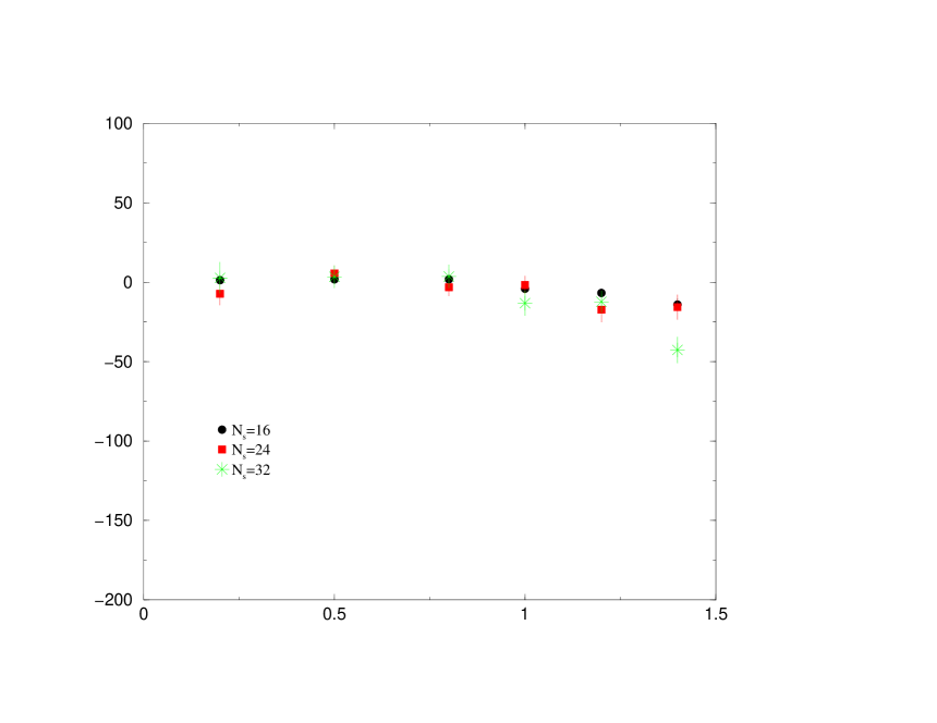
  Figure 4: Limit at large $N_{s}$ of $\rho$ for $\beta<\beta_{c}$, $SU(2)$ gauge group.

• .In the region $\beta>\beta_{c}$ the dependence of $\rho$ on $N_{s}$ can be studied . It is found (see fig.5)

  $$\rho=-kN_{s}+k^{\prime}\qquad k>0$$ (64)

  

  Figure 5: $\rho$ vs $N_{s}$ for $\beta>\beta_{c}$.

  In the limit $N_{s}\to\infty$, $\langle\mu\rangle$ is strictly zero. A direct determination of $\langle\mu\rangle$ would give zero within large errors.

• In the vicinity of $\beta_{c}$ by dimensional arguments

  $$\langle\mu\rangle=\tau^{\delta}\Phi(\frac{a}{\xi},\frac{N_{s}}{\xi})$$ (65)

  where $\xi$ is the correlation length in units of lattice spacings. $\xi$ diverges at the critical point with an index $\nu$

  $$\xi\mathop{\sim}_{\tau\to 0}\tau^{-\nu}\qquad\tau=1-\frac{T}{T_{c}}$$ (66)

  If $\xi\gg 1$ then $1/\xi\sim 0$ and

  $$\langle\mu\rangle\sim\tau^{\delta}\Phi(0,\frac{N_{s}}{\xi})\xi\mathop{\sim}_{\tau\to 0}\tau^{-\nu}$$ (67)

  One can trade $N_{s}/\xi$ with $N_{s}^{1/\nu}\tau$ and

  $$\rho=-\frac{\delta}{\tau}+N_{s}^{1/\nu}\Phi^{\prime}(0,N_{s}^{1/\nu}\tau)$$ (68)

  or

  $$\rho/N_{s}^{1/\nu}=-\frac{\delta}{\tau N_{s}^{1/\nu}}+\Phi^{\prime}(0,N_{s}^{1/\nu}\tau)$$ (69)

A scaling law results: $\rho/N_{s}^{1/\nu}$ is a universal function of $N_{s}^{1/\nu}\tau$, independent of $N_{s}$. Fig.6 shows a typical dependence of $\rho$ on $N_{s}$. Fig.7 shows the quality of scaling for SU(2). A best square fit to the data allows to determine $\beta_{c},\nu,\delta$.

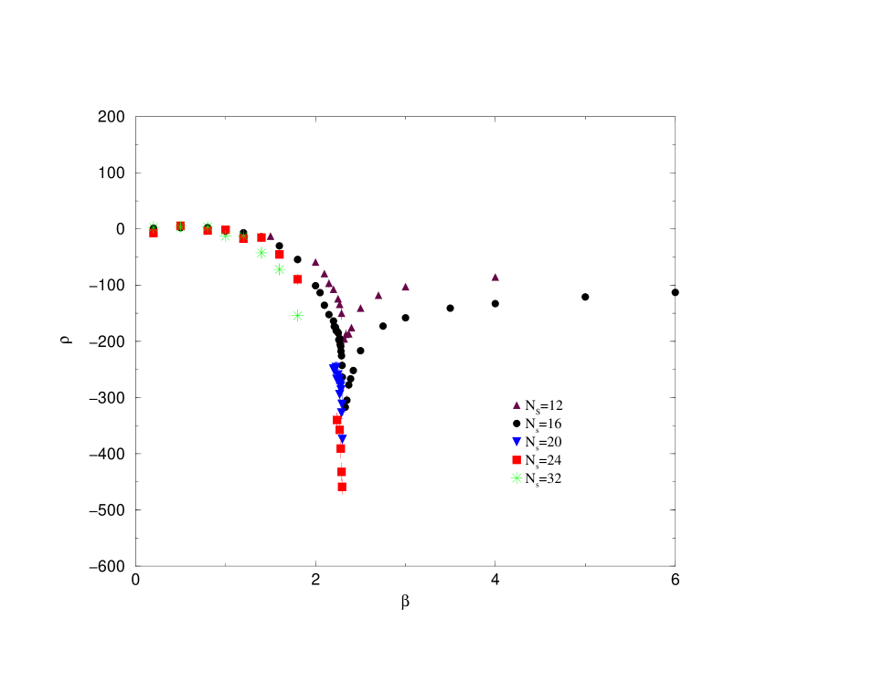
Figure 6: Volume dependence of $\rho$, pure gauge $SU(2)$, deconfinement transition.

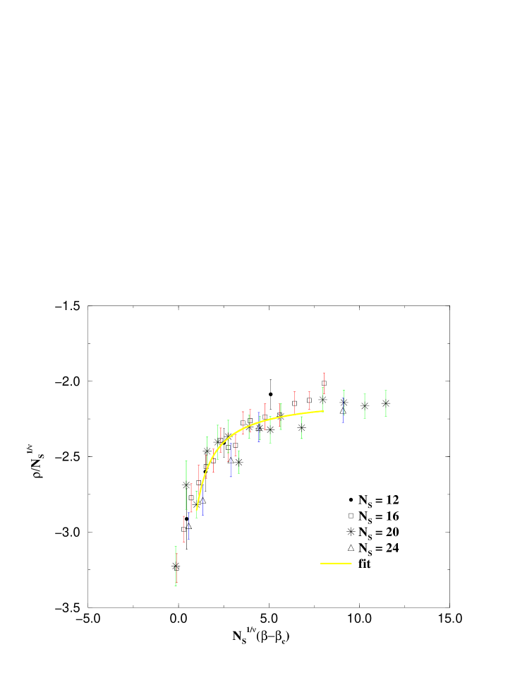
Figure 7: Scaling, eq.(69). $SU(2)$ pure gauge.

For pure gauge theory one obtains35

$$\begin{array}[]{lll}SU(2)\hskip 7.22743pt&\nu=.62(1)&\hskip 7.22743pt\delta=0.20(3)\\ SU(3)&\nu=.33(1)&\hskip 7.22743pt\delta=.50(3)\end{array}$$

The result is independent on the choice of the field used to perform the abelian projection. Confining vacuum is a dual superconductor in all abelian projections38 .

In all projections magnetic symmetry is Wigner in the deconfined phase.

Whatever the dual excitations of QCD are, they must be magnetically charged in all the abelian projections.

In QCD with dynamical quarks the same operator $\langle\mu\rangle$ can be defined ,and the corresponding $\rho=\frac{d}{d\beta}\log(\langle\mu\rangle)$ can be studied40 . Results already exist that $\langle\mu\rangle\neq 0$ in the confining phase, and $\langle\mu\rangle=0$ in the infinite volume limit. . The finite size scaling in the vicinity of the transition is on the way.

Now another scale, the quark mass enters, which was absent in the quenched case. Eq(65) -(67) become

$$\langle\mu\rangle\simeq\tau^{\delta}\Phi(\frac{1}{\xi},\frac{\xi}{N_{s}},m_{q}\xi)\mathop{\simeq}_{\xi\to\infty}\tau^{\delta}\Phi(0,N-s^{1/\nu}\tau,m_{q}N_{s}^{1/\gamma})$$ (70)

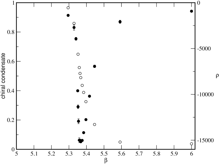
Figure 8: 2 flavour QCD. Open circles represent the chiral condensate, with the scale axis on the left. Full circles represent $\rho$, with the scale on the right. The peak of $\rho$ coincides with the drop of $\langle\bar{\psi}\psi\rangle$.

The index $\gamma$ is known. In order to determine $\nu$ one can choose values of $N_{s}$ such that $m_{q}N_{s}^{1/\gamma}$=const., and test the scaling law

$$\rho/N_{s}^{1/\nu}\sim\Phi(N_{s}^{1/\nu}\tau)$$ (71)

to determine $\nu$ and to investigate the nature of the transition. This will complete the analysis. The existing data already show,however,that dual superconductivity is the mechanism of confinement also in the presence of dynamical quarks, in agreement with the ideas of $N_{c}\to\infty$. Fig.8 shows the negative peak of $\rho$ at the same temperature where the chiral condensate drops to zero40 .

11 Concluding remarks.

Large distance QCD is an intrinsecally non perturbative system.Lattice provides a tool to investigate this regime.

Much progress has been done towards the understanding of confinement. The mechanism of confinement is definitely dual superconductivity both for pure gauge and full QCD. The dual excitations which condense to produce confinement are not yet identified:what is known is that they are magnetically charged in all abelian projections.

References

- (1) A.H.Mueller Nucl.Phys.B250(1985)327;
- (2) Review of Particle Physics E.P.J. 15 (2000)
- (3) L. B. Okun Leptons and Quarks ,North Holland (1982);
- (4) R.P.Feynman Rev.Mod.Phys. 20 (1947)267 ;
- (5) K.G. Wilson Phys.Rev.D10(1974) 2445 ;
- (6) A. Belavin, A. Polyakov, A. Schwartz, Yu. Tyupkin Phys.Lett.B205 (1988) 339;
- (7) C.G.Callan, R.F. Dashen, D.J. Gross Phys. Rev.D19 (1979) 1826;
- (8) E.V. Shuryak Rev. Mod. Phys65(1993) 1
- (9) M.A. Shifman, A.I. Vainshtein, V.I. Zakharov Nucl.Phys.B147(1979) 385,448,519 ;
- (10) K.G. Wilson Phys.Rev.D3(1971) 1818;
- (11) S. Narison Phys.Lett.B387(1996) 121;
- (12) H.G. Dosch Phys.Lett.B190(1987)555,Yu.A, Simonov Phys. Lett.B205(1988)339;
- (13) A. Di Giacomo, H. Panagopoulos Phys.Lett.B285(1992)133;
- (14) A. Di Giacomo, E. Meggiolaro, H. Panagopoulos Nucl.Phys.B483(1997)371;
- (15) M. Campostrini, A. Di Giacomo, G. Mussardo Zeits.Phys.C25(1984)173;
- (16) M. D’Elia, A. Di Giacomo, E. Meggiolaro Phys.Lett.B408(1997)315;
- (17) M. D’Elia, A. Di Giacomo, E. Meggiolaro Phys.Rev D59(1999)54503;
- (18) For a recent review and for references see: H.G. Dosch, V.I. Shevchenko, Yu.A. Simonov /hep-ph/0007223 ;
- (19) J. Engels, F. Karsch, H. Satz, I. Montvay Nucl.Phys. B205(1982) 239 ;
- (20) B. Svetitsky, L.G. Yaffe Nucl. PhysB210 (1982)423;
- (21) F. Karsch, E. Laerman Phys.Rev¿D50(1994)6954;
- (22) R.D. Pisarski, F. Wilczek Phys. Rev. D29 (1984)338
- (23) H.A. Kramers, G.H. Wannier Phys.Rev.60 (1941)252;
- (24) L.P. Kadanoff, H. Ceva Phys. Rev.B3 (1971)3918;
- (25) N. Seiberg, E. Witten Nucl. Phys.B341(1994)484;
- (26) G. Di Cecio, A. Di Giacomo, G. Paffuti, M. Triggiante Nucl. Phys.B489(1997)739;
- (27) A. Di Giacomo, D. Martelli, G. PaffutiPhys. Rev. D60(1999)094511;
- (28) G. ’tHooft Nucl. Phys.B190(1981)455;
- (29) G. ’tHooft High Energy Physics EPS International Conference Palermo 1975 , A.Zichichi ed. ,S. Mandelstam Phys. Rep. 23C(1976)245;
- (30) G. ’tHooft Nucl. Phys.B138(1978)1
- (31) L. Del Debbio, A. Di Giacomo, B. Lucini Nucl. Phys. B594(2001)287;
- (32) L. Del Debbio, A. Di Giacomo, B. Lucini Phys. Lett. B500(2001)326;
- (33) S. Weinberg Progr. Theor. Phys.Suppl.86 (1986)43;
- (34) V.L. Ginzburg, L. Landau Zh.Exp.Teor.Fiz.20 (1950)1064;
- (35) S. Coleman Erice Summer School 1981 Plenum Press,A. Zichichi ed.;
- (36) L. Del Debbio, A. Di Giacomo, G. Paffuti, P. Pieri Phys. Lett.B355(1995)255;
- (37) A. Di Giacomo, B. Lucini, L. Montesi, G. Paffuti Phys. Rev.D61(2000)034503,034504 ;
- (38) J.M. Carmona, M. D’Elia, A. Di Giacomo, B. Lucini,G. Paffuti Phys. Rev.D64(2001)114507;
- (39) T.D. Lee, C.N. Yang Phys.Rev¿87(1952)404;
- (40) J.M. Carmona, M. D’Elia, L. Del Debbio, A. Di Giacomo, B. Lucini, G. Paffuti Nucl. Phys B106 Proc.Suppl. (2002) 607 and in preparation