CERN-TH/2001-262
October 2001
Lattice QCD on PCs? 

Abstract

Current PC processors are equipped with vector processing units and have other advanced features that can be used to accelerate lattice QCD programs. Clusters of PCs with a high-bandwidth network thus become powerful and cost-effective machines for numerical simulations.

1 INTRODUCTION

Parallel computers built from PC components are being increasingly used in many branches of science. The obvious advantages of such machines are that the hardware is relatively cheap and that the software environment (linux operating system, the gcc compiler suite and an implementation of the MPI communication library) complies with the established standards.

Some doubts have however been raised that PC clusters are good machines for numerical simulations of lattice QCD. According to the benchmark results presented at last year’s lattice conference [1], PC processors in fact appear to perform rather poorly in these calculations, particularly so when the lattices get reasonably big. Moreover, it remains unclear how well such clusters scale to large numbers of processors, where heat dissipation, component reliability and the network performance become limiting factors.

The main message of this talk is that lattice QCD programs can be accelerated by a large factor if use is made of the vector arithmetic unit and other enhancements of current PC processors. As a consequence (and also for various other reasons) the prospects for doing numerical simulations on PC clusters are now much brighter than they were only a year ago.

2 PC PROCESSOR PERFORMANCE

2.1 Multimedia extensions

The vector processing capabilites mentioned above have been added to the recent generations of PC processors to speed up multimedia applications. Depending on the brand and type of processor, the associated instruction sets go under the name of MMX, 3DNow!, SSE and SSE2. In most cases these instructions operate on short vectors of data in parallel and require one or two machine cycles to complete.

Evidently the number of arithmetic operations per cycle that can be performed also depends on the rate at which the data can be moved between the memory and the arithmetic units. To reduce the associated latencies, current processors support memory-to-cache prefetch instructions and streaming memory access modes, and they include a second-level cache memory that is clocked at the processor frequency.

2.2 Benchmark results

Most of the computer time in numerical simulations of lattice QCD is spent on the solution of the Dirac equation in the presence of a given background gauge field. There are different ways to solve the equation, but in all cases the program that applies the lattice Dirac operator to a prescribed fermion field is the one that dominates the execution time. The rest of the time is used for linear combinations and scalar products of Dirac fields.

Table 1: Benchmark results obtained with a $1.4$ GHz Pentium 4 processor

	$(D_{\rm w}+m_{0})\psi$	$\psi_{1}+r\psi_{2}$	$\|\psi\|^{2}$	CG
32-bit	0.93 [1503]	0.13 [363]	0.046 [1042]	2.34 [1292]
64-bit	1.71 [814]	0.26 [181]	0.097 [497]	4.40 [687]

(Execution times in $\mu$s per lattice point [speed in Mflop/s])

In table 1 some benchmark results for these basic programs are reported, for the case of a PC with $1.4$ GHz Intel Pentium 4 processor and $256$ MB of PC800 RDRAM. The two lines in this table contain the processor times required for the specified task using 32-bit or 64-bit arithmetic. In the second column, for example, the times for the application of the Wilson–Dirac operator $D_{\rm w}+m_{0}$ to a given field $\psi$ are listed.

All figures quoted in the table are for a $16^{4}$ lattice, but on larger lattices they would be practically the same, because the memory latencies in these programs are effectively masked by the use of memory-to-cache prefetch instructions and a cache-optimized data layout. To accelerate the floating-point arithmetic, extensive use has been made of the SSE2 vector instructions that are supported on the Pentium 4 processor.

Compared with the program for the Dirac operator, the linear algebra routines (columns 3 and 4 in table 1) appear to be rather slow. This can be explained by noting that these programs spend most of the time to move data from the memory to the processing units. In a typical QCD code the linear algebra programs fortunately consume only a fraction of the total time so that their influence on the overall performance of the code is limited. This is illustrated by the figures for a standard conjugate gradient iteration quoted in the last column of table 1.

The bottom line then is that, with the current generation of PC processors and if use is made of their advanced features, it is possible to achieve sustained computational speeds that are about 10 times higher than those quoted last year [1].

In the remainder of this section, the vector unit of the Pentium 4 processor and its usage are discussed in some detail. Another issue that will be addressed is the cache management. To a large extent the impressive performance of current PC processors is in fact due to improvements of the memory system.

2.3 Streaming SIMD extension (SSE)

The vector unit on the recent Intel processors (Pentium III, Pentium 4, Itanium) has 8 registers that are denoted by xmm0,...,xmm7. They are 128 bits wide and can accommodate 2 double-precision or 4 single-precision floating-point numbers. The associated machine instructions operate on these numbers in parallel, i.e. the vector unit is a Single Instruction Multiple Data (SIMD) machine (see fig. 1).

Figure 1: The SSE instruction addps xmm0,xmm1 adds the single-precision numbers in register xmm0 to those in xmm1.

All basic arithmetic operations (parallel addition, subtraction, multiplication and division) are supported and there are further instructions for data moving and shuffling. On the Pentium III only single-precision numbers can be manipulated in this way, but the Pentium 4 supports an extended instruction set, denoted by SSE2, that allows parallel double-precision and integer arithmetic to be performed in the SSE registers. In all cases the IEEE-754 standard is respected, which guarantees proper rounding and exception handling.

2.4 Programming example

When an ISO C compliant program is compiled with the gcc compiler, the generated object code will contain general purpose and x87 FPU instructions only. The SSE unit is thus not used. There is, however, a simple way to access the SSE registers from a C program and to operate on them. Let us consider the loop

for (i=0;i<100;i++)
     a[i]=b[i]+c[i];

where a, b, c are assumed to be arrays of single-precision floating-point numbers. Since there are no data dependences in this loop, we may use the addps instruction described above to do four additions at once. The code then becomes

for (i=0;i<100;i+=4)
     __asm__ __volatile__ (
         "movaps %1, %%xmm0 \n\t"
         "movaps %2, %%xmm1 \n\t"
         "addps %%xmm0, %%xmm1 \n\t"
         "movaps %%xmm1, %0"
         :
         "=m" (a[i])
         :
         "m" (b[i]),
         "m" (c[i]));

The gcc compiler understands these lines, and if they are substituted in any C program, the executable will perform all 100 additions correctly.

The syntax of the inline assembly statement __asm__ __volatile__ (..) is documented in the manual pages of the gcc compiler. It has three arguments in the present case, a[i], b[i] and c[i], which are labelled from 0 to 2. The first line "movaps ..." moves four consecutive floating-point numbers from the address of argument 1 to the SSE register xmm0. The register then contains the array elements b[i],...,b[i+3]. Similarly the second line moves c[i],...,c[i+3] to xmm1. The parallel addition is then performed and the result is finally moved from xmm1 to the array elements a[i],...,a[i+3].

This example is rather trivial, but more complicated code sequences can be rewritten in essentially the same way, with perhaps several inline assembly statements in a row. Apart from those mentioned above, many more vector instructions are supported by the Pentium 4 processor that make it possible to perform almost any calculation in the SSE registers. The complete list of SSE2 instructions, together with detailed explanations of what precisely they do, can be downloaded from the Intel web pages [2].

In lattice QCD the SU(3) matrix times vector multiplication is one of the basic operations that is worth being coded for the SSE unit. On the Pentium 4 processor an average throughput of $1.8$ single-precision floating-point operations per cycle can been achieved in this case. The performance of the double-precision code is equally impressive and reaches $0.9$ operations per cycle.

2.5 Cache management

A common limitation of current computer architectures is that the memory system is often unable to deliver the data to the processor at a sufficiently high rate to keep the arithmetic units busy. The cache memory (which is significantly faster than the main memory) serves to enhance the data availability in those cases where the same data are used more than once.

In the program that applies the Wilson–Dirac operator to a given fermion field, for example, each spinor of the input field is processed 9 times when the program runs through the lattice. So if the spinor components that are needed at the current lattice point are already in the cache memory (because they have previously been used), it takes much less time to forward them to the arithmetic units than would otherwise be required.

Table 2: Cache line sizes [byte] and memory-to-processor bandwidths [Gbyte/s]

		Cache	Theoretical	Measured
Processor	Memory type	line size	bandwidth	bandwidth
Pentium III (0.6 GHz)	SDRAM PC133	32	1.1	0.8
Athlon (1.2 GHz)	DDRAM PC266	64	2.1	1.3
Pentium 4 (1.4 GHz)	RDRAM PC800	128	3.2	2.1

Cache memories are expensive and usually too small to contain a complete lattice Dirac field. The spinors thus tend to be overwritten before they are reused. It is possible, however, to increase the cache-hit probability by dividing the lattice into small blocks that are visited one after another. This technique (which is referred to as strip-mining) is easy to implement and often results in significant speed-up factors.

In many cases the cache-hit rate can also be enhanced by explicitly moving the data to the cache memory slightly before they are going to be used. This can be achieved by inserting prefetch instructions such as

__asm__ __volatile__ (
     "prefetcht0 %0" :: "m" (*(address)));

at the appropriate places in the program. The important point to note is that these are executed “out of order”, i.e. while the arithmetic unit is busy on other data. In ideal cases the memory latencies can thus be masked almost completely.

Data are moved from the main memory to the cache memory in blocks that are referred to as cache lines. The cache line sizes and transfer rates for some of the recent PC processors and memory types are listed in table 2. When a prefetch instruction is issued, a cache line containing the byte at the specified address is moved to the cache memory. Dirac spinors occupy one or more cache lines, depending on the line size and the data alignment, and the programmer needs to take this into account to make sure that all components are prefetched.

2.6 Program portability

Inline assembly and the SSE2 instructions are system-specific and thus not as portable as an ISO C compliant code. It is conceivable that the C language will be extended to include short vector data types once the vector units become an industry standard, and it would then be left to the compiler to produce assembler code that makes use of any advanced features of the processor.

For the time being, program portability can be preserved by first writing an ISO C program for the specified task. Where this appears worth while, inline assembly code may then be added that is conditionally compiled, i.e. only when the macro SSE2 for example is defined. In this way it can be decided at compilation time whether some parts of the ISO C program are to be replaced by system-specific code or not.

2.7 FermiQCD

Programs that make use of the SSE unit along the lines described above are now part of the FermiQCD package [3]. Many macros for SU(3) vector and matrix operations in the SSE registers can be found there, and the programs may also serve to illustrate the use of prefetch instructions. The package is freely accessible and can be downloaded from a webpage at Fermilab [4].

3 NETWORK ISSUES

3.1 Commercial PC clusters

In the course of the last two years or so, fully configured rack-mounted clusters of PCs have become a commodity. These machines usually have a switched network where any node can exchange data with any other node at full speed (see fig. 2).

As will become clear below, the bandwidth of the network is a critical parameter for clusters that are intended for numerical simulations of lattice QCD. The currently preferred network for such machines is Myrinet${}^{\rm TM}\!$ [5], which provides a one-way bandwidth per channel of up to 250 Mbyte/s. Switches for 8 to 128 nodes are available, and these can, in principle, be connected to build clusters of any size.

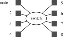
Figure 2: The nodes of a commercial PC cluster are essentially complete PCs with one or two processors. They are connected to a switch that forwards data packages between them as requested by the user programs.

3.2 How much bandwidth is needed?

Instead of developing a general formula for the required bandwidth, it may be more instructive to consider a realistic study case. So let us suppose that we have a machine with 32 nodes, each equipped with 512 MB of memory and a processor that delivers a sustained computational power of 1 Gflop/s in 32-bit arithmetic. As for the network, we assume that it provides a simultaneous bandwidth of 200 Mbyte/s per channel (the associated latencies are unimportant in the present context since the data can be transferred in large packages).

Such a machine is sufficiently big for quenched QCD simulations with Wilson fermions on a $96\times 48^{3}$ lattice. We may, for example, distribute the lattice to the nodes in such a way that each node is associated with a sublattice of size $12\times 12\times 48^{2}$ (see fig. 3). The question is then how much time is required by the communication overhead in the program that applies the Wilson–Dirac operator to a given fermion field.

When the program runs through the lattice, it reads the components of the input fermion field on the points of the local lattice and on all its boundary points. The Dirac spinors residing on the latter are stored in the memory of the logical neighbours of the current node and need to be communicated through the network before the calculation starts.

If 32-bit arithmetic is used, each Dirac spinor occupies 96 bytes of storage, and the total amount of data that must be moved to every node is thus about 11 MB. On our machine the time required for this is

$$t_{\rm com}\kern-18.00005pt =2\times{96\;{\rm byte}\over 200\;{\rm Mbyte/s}}\times\hbox{$1\over 3$}V=0.32\,\mu{\rm s}\times V,$$

where $V$ denotes the volume of the local lattice. Once all the data are available, the application of the Wilson–Dirac operator takes about $1.4\,\mu$s per lattice point, and the communication overhead is thus estimated to be 19% of the total time.

Figure 3: Cross-section of the local $12\times 12\times 48^{2}$ lattice in the $(x_{0},x_{1})$ plane (full circles). The Dirac spinors on the $4\times 12\times 48^{2}$ boundary points (open circles) need to be fetched from the neighbouring nodes.

The result of this theoretical exercise shows that current network bandwidths and processing speeds are not out of balance. It should be noted, however, that the ratio of the boundary to the bulk volume of the local lattice, and hence the communication time, tends to increase proportionally to the number of nodes that are used for a given lattice. In many cases it may, therefore, be more efficient to simulate several independent lattices in parallel.

Table 3: PC clusters dedicated for lattice QCD simulations (incomplete)

Institution	# nodes	Processor(s)	Status
Fermilab	$80$	dual Pentium III (0.7 GHz)	running
TC Dublin	$32$	dual Pentium III (1.0 GHz)	running
MPI Munich	$8$	dual Pentium III (1.0 GHz)	installation
DESY (Zeuthen)	$16$	dual Pentium 4 (1.7 GHz)	ordered
DESY (Hamburg)	$32$	Pentium 4 (1.7 GHz)	approved
Fermilab	$\sim 150$	dual Pentium 4	approved
Jlab & MIT	$128$	dual Pentium 4	approved

3.3 Possible improvements

PC processors are rapidly becoming faster, and it is clear that the network performance will have to be improved if the communication overhead is to remain small. Increasing the one-way bandwidth or having simultaneous bi-directional data transfers is certainly an option. With the current specification of the PCI bus (64 bit @ 66 MHz), transfer rates of up to 500 Mbyte/s can perhaps be reached.

An important reduction of the communication overhead might also be achieved if computation and communication can be made to overlap in time. The obvious difficulty here is that the PCI bus and the processor may be unable to access the memory concurrently with sufficient bandwidth, particularly so if the program is highly optimized.

4 PC CLUSTERS FOR LATTICE QCD

4.1 Recent installations

This year several dedicated machines have been installed or will shortly be delivered (see table 3). All these machines are commercial products that are equipped with Myrinet^TM and come with the standard software environment.

The clusters listed in the last two lines of table 3 are being funded through the Scientific Discovery through Advanced Computing (SciDAC) initiative of the US government [6]. This programme is intended to help closing the gap between nominal and actual performance of massively parallel computers and supports “research and development on scientific modeling codes, as well as on the mathematical and computing systems software that underlie these codes”.

4.2 Do PC clusters scale to Tflop/s?

Clusters with (say) 128 nodes currently reach sustained computational speeds of about 100–200 Gflop/s in lattice QCD programs. A small farm of such machines thus delivers an integrated computational power in the Tflop/s range. Having a farm of clusters is in fact not such an odd idea, since the total memory of each cluster will in many cases be sufficiently big to accommodate the lattice fields. Statistics can then be accumulated by running the same program (with different sequences of random numbers) on several machines.

Whether much larger numbers of processors can be integrated in a single cluster in a useful way is not obvious, however, and detailed studies will be needed before a solid answer to this question can be given. It seems likely, though, that the network switch will turn out to be a bottleneck when the cluster exceeds a certain critical size.

A development project, recently initiated at the University of Rome II and now supported by INFN, tries to overcome this difficulty by arranging the nodes in a logical $n\times n$ matrix. The nodes in each row and in each column are then connected to one another through $2n$ independent switches. This network geometry naturally maps to the block divisions of the physical lattice that are usually adopted. The routing of the data packages is thus simplified, and switching latencies are expected to grow only relatively slowly with the number of nodes.

4.3 Uses of small machines

When discussing computer performance and the need for ever more powerful machines, an important fact is sometimes forgotten that Giorgio Parisi pointedly described by [7]:

“In general a brute force approach to numerical simulations is not paying and a lot of ingenuity is needed in order to obtain the wanted results.”

Innovation in computational strategies and algorithms is not only essential for progress in lattice QCD, but it also represents an intellectual challenge and is certainly one of the driving forces in this field. PC clusters are well suited to try out new physical and algorithmic ideas, because they are relatively easy to use and are in many cases sufficiently powerful for significant tests to be performed in a reasonable time. Even small machines can be very useful for this kind of work on which the large-scale projects eventually depend.

Figure 4: Polyakov loop correlation function at $\beta=5.7$ and distance $r=6a\simeq 1.0\,{\rm fm}$, on a lattice of spatial size $L=12a$ and variable time extent $T$. Statistical errors are not visible on this scale.

For illustration, let us consider the Polyakov loop two-point correlation function in the SU(3) gauge theory. When the time extent $T$ of the lattice is larger than (say) $1\,{\rm fm}$, the theory is in the confinement phase and the correlation function at distance $r$ decays exponentially, roughly like

$$\langle P(r)^{\ast}P(0)\rangle\propto{\rm e}^{-\sigma A},\qquad A=rT,$$

where $\sigma\simeq 1\,{\rm GeV}/{\rm fm}$ denotes the string tension. Now if the established simulation algorithms are used, the correlation function is obtained with statistical errors that tend to be essentially independent of $A$. As a consequence the amount of computer time needed for a specified relative precision is exponentially rising and areas $A\geq 1\,{\rm fm}^{2}$ or so are practically unreachable.

It is clear that significant progress in this field can only be made if better simulation algorithms are found that lead to an exponential reduction of the statistical errors. The recently proposed multilevel algorithm [8] is of this type and works exceedingly well, at least in the case of the Wilson plaquette action.

An impressive demonstration of this is given by the data plotted in fig. 4. At the chosen coupling, the lattice spacing $a$ is about $0.17\,{\rm fm}$, and the values of $A$ covered in the plot thus reach nearly $3.5\,{\rm fm}^{2}$. In spite of the fact that the signal decays over many orders of magnitude in this range, the equivalent of no more than about $1000$ hours of processor time on a PC with $1.4$ GHz Pentium 4 processor was required to keep the statistical errors below 2% at all values of $T$.

5 CONCLUSIONS

At this point it is quite clear that PC clusters are going to be widely used for lattice QCD simulations. While smaller machines are ideal for development work and physics projects at an early stage, large clusters or farms of clusters are certainly an option for big installations, where the aim is to maximize the total computational power for a given budget.

The cost per (32-bit sustained) Mflop/s of a commercial PC cluster with Myrinet${}^{\rm TM}\!$ network is currently $3–4. In terms of cost-effectiveness, these machines are hence very competitive. How well PC clusters scale to large numbers of nodes, or whether it will be more useful to have a farm of smaller machines, remains to be seen. Further experience with both the hardware and the software will be needed, before it can be decided which is the best way to go.

Computers become more powerful at a breathtaking rate, but it seems unlikely that the hard problems in lattice QCD will gradually go away as a result of this alone. Improved numerical methods (such as those reviewed by Mike Peardon [9]) are in fact often crucial for the success of a numerical simulation project.

To explore a new approach can be fairly painful, however, if there is no reasonably fast computer around that can be freely used. PC clusters provide a good solution to this problem, and the fact that even small groups of lattice physicists may be able to afford them opens the way for more people to contribute to the development of lattice QCD.

I am indebted to Roberto Petronzio and Jarda Pech for many informative discussions on current network technologies. Thanks also go to Filippo Palombi for communicating his benchmark results for the Athlon processors and to Robert Edwards, Karl Jansen, Paul Mackenzie, Mike Peardon, Massimo Di Pierro and Peter Wegner for helpful correspondence.

References

- [1] S. Gottlieb, Nucl. Phys. B (Proc. Suppl.) 94 (2001) 833
- [2] http://www.intel.com
- [3] M. Di Pierro, FermiQCD: a toolkit for rapid development of parallel lattice QCD applications, poster at this conference; Matrix distributed processing and FermiQCD, hep-lat/0011083
- [4] http://latticeqcd.fnal.gov/software/fermiqcd /index.html
- [5] http://www.myricom.com
- [6] http://www.sc.doe.gov
- [7] G. Parisi, Principles of numerical simulations, lectures given at Les Houches (1988), in: Fields, strings and critical phenomena, eds. E. Brézin, J. Zinn-Justin (North-Holland, Amsterdam, 1989)
- [8] M. Lüscher, P. Weisz, J. High Energy Phys. 09 (2001) 010
- [9] M. Peardon, Progress in lattice algorithms, plenary talk given at this conference