Matrix elements of $\Delta S=2$ operators with Wilson fermions

D.ย Becirevic, Ph.ย Boucaud, V.ย Gimรฉnez, V.ย Lubicz, G.ย Martinellia, M.ย Papinutto Talk given by Damir Becirevic. Dip. di Fisica, Universitร  โ€œLa Sapienzaโ€ and INFN-Roma, P.le A. Moro 2, I-00185 Rome, Italy Laboratoire de Physique Thรฉorique (bรขt.210), Universitรฉ de Paris XI, 91405 Orsay Cedex, France Dep.ย de Fรญs.Teรฒrica and IFIC, Univ.ย de Valรจncia, Dr.ย Moliner 50, E-46100, Burjassot, Valรจncia, Spain Dip. di Fisica, Univ. di Roma Tre and INFN - Roma Tre, Via della V. Navale 84, I-00146 Rome, Italy Dip. di Fisica, Univ. di Pisa and INFN - Pisa, Via Buonarroti 2, I-56100 Pisa, Italy
Abstract

We test the recent proposal of using the Ward identities to compute the $K^{0}-\bar{K}^{0}$ mixing amplitude with Wilson fermions, without the problem of spurious lattice subtractions. From our simulations, we observe no difference between results obtained with and without subtractions. From the standard study of the complete set of $\Delta S=2$ operators, we quote the following (preliminary) results: $B_{K}^{\overline{\rm MS}}(2\ GeV)=0.70(10)$, $\langle O_{7}\rangle_{K\to\pi\pi}^{(I=2)}=0.10(2)(1){\rm GeV}^{3}$, $\langle O_{8}\rangle_{K\to\pi\pi}^{(I=2)}=0.49(6)(0){\rm GeV}^{3}$.

The main problem in lattice computations of the $4$-fermion $\Delta F=2$ operators with Wilson fermions is related to spurious mixing among dimension-six operators. For example, chiral symmetry ensures that the operator responsible for the indirect $CP$-violation in the $K^{0}-\bar{K}^{0}$ system, Q1=sยฏaโ€‹ฮณฮผโ€‹(1โˆ’ฮณ5)โ€‹daโ€‹sยฏbโ€‹ฮณฮผโ€‹(1โˆ’ฮณ5)โ€‹dbsubscript๐‘„1superscriptยฏ๐‘ ๐‘Žsubscript๐›พ๐œ‡1subscript๐›พ5superscript๐‘‘๐‘Žsuperscriptยฏ๐‘ ๐‘subscript๐›พ๐œ‡1subscript๐›พ5superscript๐‘‘๐‘Q_{1}=\bar{s}^{a}\gamma_{\mu}(1-\gamma_{5})d^{a}\ \bar{s}^{b}\gamma_{\mu}(1-\gamma_{5})d^{b}, renormalizes multiplicatively. Since the Wilson term explicitly breaks chiral symmetry, $Q_{1}$ mixes instead with all the other $\Delta S=2$ operators including

Q2=sยฏaโ€‹(1โˆ’ฮณ5)โ€‹daโ€‹sยฏbโ€‹(1โˆ’ฮณ5)โ€‹dbsubscript๐‘„2superscriptยฏ๐‘ ๐‘Ž1subscript๐›พ5superscript๐‘‘๐‘Žsuperscriptยฏ๐‘ ๐‘1subscript๐›พ5superscript๐‘‘๐‘\displaystyle Q_{{}_{2}}=\bar{s}^{a}(1-\gamma_{5})d^{a}\ \bar{s}^{b}(1-\gamma_{5})d^{b}\; (1)
j Q3=sยฏaโ€‹(1โˆ’ฮณ5)โ€‹dbโ€‹sยฏbโ€‹(1โˆ’ฮณ5)โ€‹dasubscript๐‘„3superscriptยฏ๐‘ ๐‘Ž1subscript๐›พ5superscript๐‘‘๐‘superscriptยฏ๐‘ ๐‘1subscript๐›พ5superscript๐‘‘๐‘Ž\displaystyle Q_{{}_{3}}=\bar{s}^{a}(1-\gamma_{5})d^{b}\ \bar{s}^{b}(1-\gamma_{5})d^{a}\; (2)
j Q4=sยฏaโ€‹(1โˆ’ฮณ5)โ€‹daโ€‹sยฏbโ€‹(1+ฮณ5)โ€‹dbsubscript๐‘„4superscriptยฏ๐‘ ๐‘Ž1subscript๐›พ5superscript๐‘‘๐‘Žsuperscriptยฏ๐‘ ๐‘1subscript๐›พ5superscript๐‘‘๐‘\displaystyle Q_{{}_{4}}=\bar{s}^{a}(1-\gamma_{5})d^{a}\ \bar{s}^{b}(1+\gamma_{5})d^{b}\; (3)
j Q5=sยฏaโ€‹(1โˆ’ฮณ5)โ€‹dbโ€‹sยฏbโ€‹(1+ฮณ5)โ€‹dasubscript๐‘„5superscriptยฏ๐‘ ๐‘Ž1subscript๐›พ5superscript๐‘‘๐‘superscriptยฏ๐‘ ๐‘1subscript๐›พ5superscript๐‘‘๐‘Ž\displaystyle Q_{{}_{5}}=\bar{s}^{a}(1-\gamma_{5})d^{b}\ \bar{s}^{b}(1+\gamma_{5})d^{a}\; (4)

where the superscripts denote color indices. The spurious mixing may seriously modify the chiral behavior of the operator $Q_{1}$ and hence need to be subtracted away, $Q_{1}^{(sub.)}(a)=Q_{1}(a)+\Delta_{i}(a)Q_{i}(a)$ $(i=2,\dots,5)$. After completing the subtraction procedure of the โ€œwrong chiralityโ€ operators, the bare lattice regularized operator $Q_{1}^{(sub.)}(a)$ must be multiplicatively renormalized (like in the continuum): $\hat{Q}_{1}(\mu)=Z_{11}(\mu a)Q_{1}^{(sub.)}(a)$. A complete programme of renormalization of the operators $Q_{1-5}$ requires the computation of 9 renormalization and 16 subtraction constants. This can be done perturbatively (see ref.ย [1]), but since the ๐’ชโ€‹(ฮฑs)๐’ชsubscript๐›ผ๐‘ {\cal O}(\alpha_{s}) terms are uncomfortably large, a non-perturbative determination of these 25 constants is mandatory. A theoretically simple method to implement the renormalization in the so-called (Landau)RI/MOM scheme has been summarized in ref.ย [2]. In practice this programme is, however, quite complicated. Even more so since the procedure included also the necessity to subtract the Goldstone boson (single and double pole) contributionsย [3, 4, 5]. That may cast doubts on the reliability of the method, i.e. on the level of control of the systematic errors. To address that issue, one needs a method allowing a computation without the necessity to subtract mixing with operators of the wrong chirality, and compare the results to the ones obtained by using the standard method (with subtractions). Recently, two such proposals appeared: twisted mass QCDย [6] (see [7] for the first numerical results), and method of the Ward identitiesย [8] which we use is what follows.

1 Ward Identity Methodย [8]

The method is extremely simple and to summarize it in a few lines we write the parity even (PE) operator $Q_{1}$ as $Q_{1}=VV+AA$, in an obvious notation. For symmetry reasons, unlike the PE, the parity odd (PO) operators do not suffer from spurious mixings (i.e. $\Delta_{ij}^{PO}(a)=0$). It is then possible to apply the Ward identity on the matrix element of the PO operator, ${\cal Q}_{1}=AV+VA$, to get the matrix element of the PE one, $Q_{1}$. By applying the chiral rotation around the third axis in isospace, $\delta u=\gamma_{5}u$, $\delta d=-\gamma_{5}d$ ($m_{u}=m_{d}\equiv m$), on $\langle P(\vec{x},t_{x}){\cal Q}_{1}(0)P(\vec{y},t_{y})\rangle$, one arrives at

mโ€‹โŸจโˆ‘xโ†’,yโ†’,zโ†’,tzฮ โ€‹(zโ†’,tz)โ€‹Pโ€‹(xโ†’,tx)โ€‹๐’ฌ1โ€‹(0)โ€‹Pโ€‹(yโ†’,ty)โŸฉ=๐‘šdelimited-โŸจโŸฉsubscriptโ†’๐‘ฅโ†’๐‘ฆโ†’๐‘งsubscript๐‘ก๐‘งฮ โ†’๐‘งsubscript๐‘ก๐‘ง๐‘ƒโ†’๐‘ฅsubscript๐‘ก๐‘ฅsubscript๐’ฌ10๐‘ƒโ†’๐‘ฆsubscript๐‘ก๐‘ฆabsent\displaystyle m\langle\displaystyle{\sum_{\vec{x},\vec{y},\vec{z},t_{z}}}\Pi(\vec{z},t_{z})\ P(\vec{x},t_{x})\ {\cal Q}_{1}(0)\ P(\vec{y},t_{y})\rangle= (5)
$\displaystyle\langle\displaystyle{\sum_{\vec{x},\vec{y}}}P(\vec{x},t_{x})\ Q_{1}(0)\ P(\vec{y},t_{y})\rangle+{\rm(rot.\ sources)}$ (6)

where the terms arising from the rotation of the source operators P=dยฏโ€‹ฮณ5โ€‹s๐‘ƒยฏ๐‘‘subscript๐›พ5๐‘ P=\bar{d}\gamma_{5}s, vanish due to the symmetry under the charge conjugation. In the above identity, ฮ =dยฏโ€‹ฮณ5โ€‹dโˆ’uยฏโ€‹ฮณ5โ€‹uฮ ยฏ๐‘‘subscript๐›พ5๐‘‘ยฏ๐‘ขsubscript๐›พ5๐‘ข\Pi=\bar{d}\gamma_{5}d-\bar{u}\gamma_{5}u. Thus, to get an informations on the r.h.s., we compute the l.h.s. where the operator ${\cal Q}_{1}$ renormalizes only multiplicatively. Moreover, $Z_{P}(\mu)$, which renormalizes the density ฮ ฮ \Pi, cancels against the one appearing in the mass renormalization constant, $Z_{m}(\mu)=Z_{A}/Z_{P}(\mu)$, so that only $Z_{A}$ is required. We computed the l.h.s. of the above identity on the lattice at $\beta=6.0$ ($16^{3}\times 52$) and at $\beta=6.2$ ($24^{3}\times 64$). Results of both simulations were presented at the conference. Due to the lack of space, here we present only the results obtained on the finer lattice ($\beta=6.2$, 200 configurations), where we work with $\kappa_{q}\in\{0.1339,0.1344,0.1349,0.1352\}$. Complete results with accompanying details will be presented in ref.ย [9].

To confront the two methods, we studied the following ratios:

โ„›1โ€‹(tx)=mโ€‹โŸจโˆ‘xโ†’,yโ†’,zโ†’,tzฮ โ€‹(zโ†’,tz)โ€‹Pโ€‹(xโ†’,tx)โ€‹๐’ฌ^1โ€‹(0)โ€‹Pโ€‹(yโ†’,ty)โŸฉZAโ€‹โŸจโˆ‘xโ†’Pโ€‹(xโ†’,tx)โ€‹Pโ€‹(0)โŸฉโ€‹โŸจโˆ‘yโ†’Pโ€‹(yโ†’,ty)โ€‹Pโ€‹(0)โŸฉ,subscriptโ„›1subscript๐‘ก๐‘ฅ๐‘šdelimited-โŸจโŸฉsubscriptโ†’๐‘ฅโ†’๐‘ฆโ†’๐‘งsubscript๐‘ก๐‘งฮ โ†’๐‘งsubscript๐‘ก๐‘ง๐‘ƒโ†’๐‘ฅsubscript๐‘ก๐‘ฅsubscript^๐’ฌ10๐‘ƒโ†’๐‘ฆsubscript๐‘ก๐‘ฆsubscript๐‘๐ดdelimited-โŸจโŸฉsubscriptโ†’๐‘ฅ๐‘ƒโ†’๐‘ฅsubscript๐‘ก๐‘ฅ๐‘ƒ0delimited-โŸจโŸฉsubscriptโ†’๐‘ฆ๐‘ƒโ†’๐‘ฆsubscript๐‘ก๐‘ฆ๐‘ƒ0\displaystyle{\cal R}_{1}(t_{x})={m\ \langle\displaystyle{\sum_{\vec{x},\vec{y},\vec{z},t_{z}}}\Pi(\vec{z},t_{z})\ P(\vec{x},t_{x})\ \hat{\cal Q}_{1}(0)\ P(\vec{y},t_{y})\rangle\over Z_{A}\ \langle\displaystyle{\sum_{\vec{x}}}P(\vec{x},t_{x})P(0)\rangle\langle\displaystyle{\sum_{\vec{y}}P(\vec{y},t_{y})P(0)\rangle}},
$\displaystyle{\cal R}_{2}(t_{x})={\langle\displaystyle{\sum_{\vec{x},\vec{y}}}P(\vec{x},t_{x})\ \hat{Q}_{1}(0)\ P(\vec{y},t_{y})\rangle\over Z_{A}^{2}\ \langle\displaystyle{\sum_{\vec{x}}}P(\vec{x},t_{x})P(0)\rangle\langle\displaystyle{\sum_{\vec{y}}P(\vec{y},t_{y})P(0)\rangle}},$

where, when needed, we used the non-perturbatively determined renormalization and subtraction constants. In the above formulae the time $t_{y}$ has been fixed, $t_{x}$ is left free and $t_{z}$ has been summed over all lattice. The role of denominators is to eliminate the usual exponential terms in the numerator.
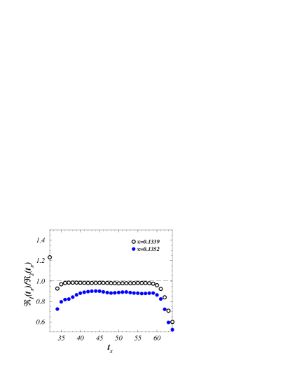
Refer to caption
Figure 1: Method without subtractions (${\cal R}_{1}(t_{x})$) is confronted to the standard one โ€“ with subtractions (${\cal R}_{2}(t_{x})$). Subtraction constants are computed non-perturbatively.

First, we observe that the plateaus for the ratio โ„›1โ€‹(tx)subscriptโ„›1subscript๐‘ก๐‘ฅ{\cal R}_{1}(t_{x}) exist and they are good for all the quark masses used in our study (seeย [9]). Second, by using the method without (โ„›1โ€‹(tx)subscriptโ„›1subscript๐‘ก๐‘ฅ{\cal R}_{1}(t_{x})) and with (โ„›2โ€‹(tx)subscriptโ„›2subscript๐‘ก๐‘ฅ{\cal R}_{2}(t_{x})) subtractions, we get the results very consistent with each other. In fig.ย 1 we show the ratio โ„›1/โ„›2subscriptโ„›1subscriptโ„›2{\cal R}_{1}/{\cal R}_{2} for the smallest and the largest of our quark masses. From the observation that (on the plateau) for all our masses we get 0.89โ‰คโ„›1/โ„›2โ‰ค0.980.89subscriptโ„›1subscriptโ„›20.980.89\leq{\cal R}_{1}/{\cal R}_{2}\leq 0.98, we conclude that the agreement of the two methods is satisfactory. Note that results of two methods have different Oโ€‹(a)๐‘‚๐‘ŽO(a) effects. 
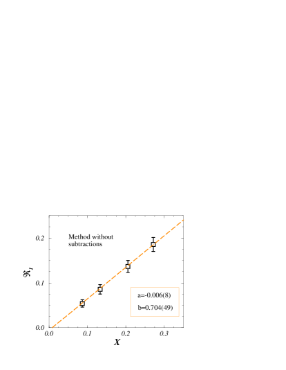
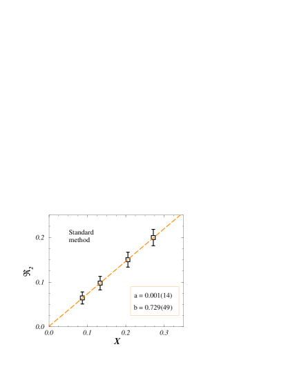
We checked that the chiral behavior for the matrix element โŸจQ1โ€‹(ฮผ)โŸฉdelimited-โŸจโŸฉsubscript๐‘„1๐œ‡\langle Q_{1}(\mu)\rangle, as extracted by using either of the two methods, is good, i.e. that โ„›2โ€‹(tx)โ†’0โ†’subscriptโ„›2subscript๐‘ก๐‘ฅ0{\cal R}_{2}(t_{x})\to 0 when mqโ†’0โ†’subscript๐‘š๐‘ž0m_{q}\to 0 (see fig.ย 2). In addition, we performed the analysis of the data (w/o subtractions) when a small momentum is given to the external sources (โ€œkaonsโ€). After following the usual extrapolation proceduresย [10], we get

$\displaystyle\hskip 34.1433ptB_{K}^{{\overline{\rm MS}}}=0.70(10)\,.$ (7)

This error can be substantially reduced if the computation is made at several lattice spacing so that the momentum injections to the external kaons (for which the signals are noisier) are not neededย [9].

2 $B$-parameters of the SUSY operators

As seen in the previous section, the two methods give very consistent results which makes us more confident that systematic errors introduced by using the standard method (with subtraction and renormalization constants computed non-perturbatively), are indeed under control. We used the standard method to compute the matrix elements for the SUSY operators listed in eq.ย (1). They are parameterized as

$\displaystyle\langle\bar{K}^{0}|\hat{Q}_{2-5}(\mu)|K^{0}\rangle=B_{2-5}(\mu)\ c_{2-5}\times$ (8)
ร—โŸจKยฏ0|sยฏโ€‹ฮณ5โ€‹dโ€‹(ฮผ)โ€‹0โŸฉโ€‹โŸจ0|sยฏโ€‹ฮณ5โ€‹dโ€‹(ฮผ)|K0โŸฉ,absentinner-productsuperscriptยฏ๐พ0ยฏ๐‘ subscript๐›พ5๐‘‘๐œ‡0quantum-operator-product0ยฏ๐‘ subscript๐›พ5๐‘‘๐œ‡superscript๐พ0\displaystyle\hskip 19.91692pt\times\langle\bar{K}^{0}|\bar{s}\gamma_{5}d(\mu)0\rangle\langle 0|\bar{s}\gamma_{5}d(\mu)|K^{0}\rangle\ , (9)

where $c_{2}=-5/3$, $c_{3}=1/3$, $c_{4}=2$, $c_{5}=2/3$, so that the corresponding $B$-parameters are unity in the vacuum saturation approximation. Each $B_{i}$-parameter is computed by replacing $Q_{1}\to Q_{i}$ in ${\cal R}_{2}(t_{x})$ and dividing by $Z_{P}^{2}(\mu)$ instead of $Z_{A}^{2}$. Conversion from the RI/MOM scheme to the ${\overline{\rm MS}}$(NDR) scheme of ref.ย [11] is made in perturbation theory with NLO accuracy. By linearly interpolating to the physical kaon mass, we obtain the following values:

$\displaystyle B_{2}^{\overline{\rm MS}}(2\ {\rm GeV})=0.64(5)(2)\,,$ (10)
$\displaystyle B_{3}^{\overline{\rm MS}}(2\ {\rm GeV})=0.97(8)(12)\,,$ (11)
$\displaystyle B_{4}^{\overline{\rm MS}}(2\ {\rm GeV})=0.87(6)(3)\,,$ (12)
$\displaystyle B_{5}^{\overline{\rm MS}}(2\ {\rm GeV})=0.58(5)(1)\,,$ (13)

which, together with $B_{1}$ given in eq.ย (7), gives a complete set of $B$-parameters of $\Delta S=2$ operators needed for the analysis of the SUSY effects in the $K^{0}-\bar{K}^{0}$ mixing amplitudeย [12].

3 Very briefly on $\langle(\pi\pi)_{I=2}|Q_{7,8}(\mu)|K^{0}\rangle$

From the results of the previous section, one may get the useful information on the $\Delta I=3/2$ amplitude of the $K\to\pi\pi$ decay. After extrapolating to the chiral limit, the relevant bag parameters are: $B_{5}^{\chi}\equiv B_{7}^{\overline{\rm MS}}(2{\rm GeV})=0.46(6)(2)$, and $B_{4}^{\chi}\equiv B_{8}^{\overline{\rm MS}}(2{\rm GeV})=0.82(7)(3)$. To predict the matrix elements in physical units, we will use the recipe of ref.ย [13], which avoids the multiplication by the quark condensate (squared) and replaces it by the multiplication by $m_{\rho}^{2}f_{\pi}^{2}$. Using that strategy, in the ${\overline{\rm MS}}$(NDR) scheme of ref.ย [11], we obtain:

$\displaystyle\langle\pi^{+}|O_{7}^{3/2}(2\ {\rm GeV})|K^{+}\rangle=-0.0193(33)(13)\ {\rm GeV}^{4},$ (14)
$\displaystyle\langle\pi^{+}|O_{8}^{3/2}(2\ {\rm GeV})|K^{+}\rangle=-0.092(10)(0)\ {\rm GeV}^{4}.$

These results, after using the soft pion theorem $\langle(\pi\pi)_{I=2}|O_{7,8}|K^{0}\rangle=-\langle\pi^{+}|O^{3/2}_{7,8}|K^{+}\rangle/f_{\pi}\sqrt{2}$ย [14], lead to

$\displaystyle\langle O_{7}(2\ {\rm GeV})\rangle_{K\to\pi\pi}^{(I=2)}=0.104(18)(7)\ {\rm GeV}^{3}$ (15)
$\displaystyle\langle O_{8}(2\ {\rm GeV})\rangle_{K\to\pi\pi}^{(I=2)}=0.49(6)(0)\ {\rm GeV}^{3},$

which can be compared to the preliminary estimates of the SPQcdR collaboration, $\langle O_{7}(2\ {\rm GeV})\rangle_{K\to\pi\pi}^{(I=2)}=0.021(11)~{}{\rm GeV}^{3}$ and $\langle O_{8}(2\ {\rm GeV})\rangle_{K\to\pi\pi}^{(I=2)}=0.53(6)~{}{\rm GeV}^{3}$, as obtained by directly computing $K\to\pi\pi$ matrix elements on the lattice. For comparison with other groups and other approaches, see ref.ย [15].

References

  • [1] R.ย Gupta et al.,[hep-lat/9611023].
  • [2] A.ย Donini et al.,[hep-lat/9902030].
  • [3] J.R.ย Cudell et al.,[hep-lat/9810058].
  • [4] C.ย Dawson et al.,[hep-lat/0011036].
  • [5] M.ย Papinutto, at this conference.
  • [6] R.ย Frezzotti et al.,[hep-lat/0101001].
  • [7] C.ย Peรฑa et al.,[hep-lat/0110097].
  • [8] D.ย Becirevic et al.,[hep-lat/0005013].
  • [9] S.P.Qcd R, in preparation.
  • [10] D.ย Becirevic et al.,[hep-lat/0012009].
  • [11] A.ย Buras et al.,[hep-ph/0005183].
  • [12] F.ย Gabbiani et al.,[hep-ph/9604387].
  • [13] L.ย Giusti, et al.,[hep-lat/9910017].
  • [14] C.ย Bernard, et al., Phys.Rev.D32 (1985) 2343.
  • [15] G.ย Martinelli, [hep-ph/0110023].
Refer to caption
Refer to caption
Figure 2: Chiral behavior of the matrix element of the operator ${\hat{Q}}_{1}(\mu\approx 1/a)$ as obtained by using the methods without (left figure) and with subtractions (right figure). The values of the fit parameters ${\cal R}=a+bX$ are also given ($X\propto m_{q}$, see ref.ย [10] for the precise definition).